Characteristics of Carbonaceous PM2.5 in a Small Residential City in Korea


1
Department of Environmental Science, Kangwon National University, Chuncheon 24341, Kangwon-do, Korea
2
Research Center, SinHaeng Construction Co., Ltd., Gwangmyung 13976, Gyeonggi-do, Korea
3
Air quality Research Division, National Institute of Environmental Research, Incheon 22689, Korea
*
Author to whom correspondence should be addressed.
Atmosphere 2018, 9(12), 490; https://doi.org/10.3390/atmos9120490
Submission received: 5 November 2018
/
Revised: 30 November 2018
/
Accepted: 6 December 2018
/
Published: 11 December 2018
(This article belongs to the Special Issue Air Quality in the Asia-Pacific Region)
Abstract
:PM2.5 has been a serious issue in South Korea not only in urban and industrial areas but also in rural and background areas. In this study, PM2.5 and its carbonaceous compounds including organic carbon (OC), elemental carbon (EC), water-soluble organic carbon (WSOC), and polycyclic aromatic hydrocarbons (PAHs) were collected and analyzed in a small residential city. The PM2.5 concentration frequently exceeded the national ambient air quality standard during the spring and the winter, which often occurred concurrently with fog and mist events. Over the whole sampling period, both OC and the OC/EC ratio were considerably higher than the ratios in other cities in Korea, which suggests that sources other than vehicular emissions were important. The top 10% of OC/EC ratio samples could be explained by regional and long-range transport because there was a strong correlation between primary and secondary organic carbon. However, biomass combustion was likely to account for the consistently high OC concentration due to a strong correlation between WSOC and primary OC as well as the diagnostic ratio results of PAHs.
1. Introduction
It has been proven that fine particles (PM2.5) have raised various problems including adverse health effects, low visibility, and intensified climate change [1]. One of the major constituents of PM2.5 are carbonaceous compounds, which are often classified into organic carbon and elemental carbon in an operational definition. EC is emitted primarily from combustion processes while OC can be formed secondarily through homogeneous gas-phase oxidation, gas-aerosol partitioning, and/or heterogeneous oxidation of volatile organic compounds. It can also be directly emitted from primary sources including fossil fuel combustion, biomass burning, and biogenic emissions [2]. OC can be divided into two sub-groups such as water-soluble organic carbon and water insoluble organic carbon, which also tends to follow the classification of pure hydrocarbon organic aerosol and oxygenated organic aerosol [3,4]. WSOC is either directly emitted from biomass burning [5,6] or formed secondarily in atmospheric processes through gas-to-particle conversion after the oxidation of volatile organic compounds to semi-volatile forms [5,7,8]. In many previous studies, WSOC was strongly correlated with secondary inorganic compounds such as ammonium nitrate (NH4NO3) as well as secondary organic compounds such as oxalate [9]. Some studies have also suggested that the secondary organic aerosol (SOA), oxygenated organic aerosol (OOA), and WSOC show very similar chemical characteristics, which indicates that WSOC can serve as a proxy for secondary OC.
Polycyclic aromatic hydrocarbons (PAHs) are the one type of primary OC that have a minimum of two benzene rings and are generated from incomplete combustion processes including the pyrolysis of fossil fuels, bio-incineration, domestic heating, and waste incineration [10,11]. PAHs are semi-volatile organic compounds (SVOCs), which are present in the atmosphere in both the gas and particulate phases. The low and middle molecular weight PAHs have high vapor pressures and tend to exist in the gas phase while the high molecular weight PAHs have low vapor pressures and tend to exist in the particulate phase. The US Environmental Protection Agency (US EPA) has designated 16 PAHs that have a detrimental effect on humans such as carcinogenesis. In particular, benzo [a] pyrene is known to exhibit the strongest toxicity among PAHs and is classified as a substance that can cause cancer in humans and animals along with benzo[a]anthracene, chrysene, indeno[1,2,3-c,d]pyrene, and benzo[b]fluoranthene [12].
In South Korea, the atmospheric levels of representative primary pollutants such as carbon monoxide and sulfur dioxide have been efficiently reduced due to the adoption of policies including fuel conversion and tightened emissions standards. However, the concentration of PM2.5 is still two or three times higher than those found in the United States, Japan, and most European countries [13]. In Korea, the PM2.5 concentrations are relatively spatially consistent, which means that the concentration often exceeds the national ambient air quality standard (NAAQS) even in background areas possibly due to the long-range transport of pollutants originating from China. With the industry developing at a rapid rate in China, air pollutant transport has been creating serious issues in nearby countries such as Korea and Japan. Chuncheon represents a small-sized or medium-sized city composed of residential areas where no large industrial emissions sources are located. According to the National Emissions Inventory, the emission rate of PM2.5 in this city is very low compared with rates for other major cities. However, its atmospheric concentrations have been similar to or even higher than those in other major cities including Seoul, which is the capital of Korea, in recent years [14,15]. Measurements from the national monitoring network showed that the concentrations of PM10, PM2.5, O3, and CO in Chuncheon were higher than or similar to those in urban and industrial cities while NO2 and SO2, the primary pollutants from fossil fuel combustion, showed relatively low concentrations in Chuncheon, which indicates that the pollutants are formed secondarily during long-range transport to this city. A previous study showed that OC was higher in Chuncheon than in other cities of Korea [16]. The main objective of this study is to identify the major causes for the elevated OC concentration in this city. There can be a few hypotheses to explain the high PM2.5 and the high OC contribution to the PM2.5 mass in this city. First, regional-range or long-range transport from urban areas may be important and aged organic carbon becomes predominant. Second, there may be some primary sources with high OC emission rates that have been omitted by the National Emissions Inventory. Third, the in-situ production of secondary OC may be important because of the unique meteorological features of this city. In this study, PM2.5 samples were collected and their OC, EC, WSOC, and PAH concentrations were measured. In addition, possible sources of carbonaceous aerosols were identified by using various methods to test the hypotheses listed above.
2. Materials and Methods
2.1. Sampling and Analysis
The concentrations of PM2.5 and its carbonaceous compounds were measured for 24 h every 3 days in Chuncheon, Korea from April 2012 to August 2015. The city is located approximately 100 km northeast of the metropolitan region of Korea (Seoul) and major industrial regions (Incheon) (Figure 1). Therefore, PM2.5 emitted in the urban and industrial areas of Korea and China can be transported into the city of Chuncheon with westerly winds. A PM2.5 sequential sampler (PMS-103, APM Engineering, Korea) and an FH 95 (Andersen) were deployed for collecting PM2.5 mass and carbonaceous compounds, respectively, on the roof of a four-story building on the campus of Kangwon National University (37.8695° N, 127.7445° E). The PM2.5 sampling followed the US EPA Compendium Method IO-4.2 [17]. A 47 mm Teflon filter (Pall Life Sciences, Pall Corporation, New York, NY, USA) was placed in a clean Teflon cassette with a flow rate of 16.7 Lpm for sampling PM2.5 mass. The Teflon filters were stored in controlled conditions of temperature (20 °C) and relative humidity (50%) for at least 24 h and then weighed using an analytical balance (Sartorius CP225D, readability = 10−5 g) before and after sampling.
To collect carbonaceous compounds in PM2.5, a 47 mm quartz filter that had been baked in a furnace at 450 °C for 12 h was used. After sampling, a small piece (1.5 cm2) was punched out from the quartz filter and analyzed using the NIOSH (National Institute of Occupational Safety and Health) method 5040 [18] to measure OC and EC concentrations. NIOSH 5040 protocol for thermal-optical analysis was used in which a sample is heated in pure helium (He), which was followed by a temperature decrease, the addition of 2% oxygen (O2) to the He atmosphere, and then heated to 870 °C. Some organic carbonaceous aerosols that are not volatilized in the He stage remain in the filter as a carbonized or pyrolyzed fraction, which is called pyrolyzed OC (PC). Thus, the total OC is calculated by adding the PC to the amount of carbon measured at the He stage and the total EC is calculated by subtracting the PC from the carbon measured at the He-O2 stage. Experimental parameters for the thermal/optical analytical protocol are shown in Table 1. OC is fragmentized into OC1, OC2, OC3, OC4, and PC. EC is fragmentized into EC1 to EC6. The remaining portion of the quartz filter was placed into a conical tube filled with 30 mL of deionized water and extracted using a sonicator for 1 h. The extract was filtered using a 0.45 μm PTFE syringe filter (Pall Life Sciences) and WSOC was quantified using a TOC analyzer (Sievers 5310C Laboratory, Boulder, CO, USA). WSOC concentrations were measured only from February 2015 to July 2015 (N = 66).
PM2.5 samples for PAHs were sampled from December 2014 to August 2015 using a PMS-103 sampler with a pre-baked 47 mm quartz filter at a flow rate of 16.7 Lpm (N = 66). After sampling, the filters were wrapped in aluminum foil to prevent any artifact derived from exposure to sunlight and stored in a freezer to await the analysis. The filters were cut into 6 pieces and placed in amber glass vials containing 5 mL of acetonitrile (HPLC grade) and extracted twice in an ultra-sonicator for 30 min. The extracts were then filtered by using a 0.45 μm PTFE syringe filter (Pall Life Sciences) and then reduced to 1 mL at 45 °C using a Turbo storm vacuum pump (SCINCO, Korea) under a UHP N2 gas stream. The concentrated solution was transferred into 2 mL vials and concentrated to the final volume of 0.5 mL using a mini-Vap 6-port concentrator (SUPELCO). HPLC-UV (Waters 996 PDA at 254 nm) was used to analyze fluorene (Flu), phenanthrene (Phe), and anthracene (Ant) while chrysene (Chr) and HPLC-FLD (Waters 2475 FLD at 340 nm (ex), 425 nm (em)) was used for fluoranthene (Flt), pyrene (Pyr), benzo[a]anthracene (BaA), benzo[b]fluoranthene (BbF), benzo[k]fluoranthene (BkF), benzo[a]pyrene (BaP), dibenzo[a,h]anthracene (DaA), indeno[1,2,3-c,d]pyrene (IcP), and benzo[ghi]perylene (BgP) [19].
Meteorological data including temperature, wind speed, wind direction, relative humidity, and solar radiation were also measured every 5 min at the sampling site using a meteorological tower (Vintage Pro2, DAVIS Inc., California, CA, USA).
2.2. QA/QC
Field blanks were collected after every 6th sample while the method detection limit (MDL) was calculated as 3 times the standard deviation of the field blanks. Concentration values less than the MDL were substituted with 0.5 × MDL. The relative percent differences (RPDs) of triplicate analyzes were 6.5%, 9.4%, and 1.8% for OC (organic carbon), EC (elemental carbon), and WSOC (water-soluble organic carbon), respectively. A five-point calibration curve was obtained to quantify each PAH species. The instrument detection limit was calculated as three times the standard deviation of the concentrations determined by analyzing a 0.2 ng/mL standard solution 5 times. RPDs for PAHs were calculated by analyzing identical samples 5 times. All QA/QC results including recovery rates are shown in Table 2. The recovery rates were in the acceptable range suggested by the US EPA [20]. Anthracene was excluded due to the low recovery rate and 12 PAHs in total were quantified.
2.3. Statistical Analysis
Most of the data in this study are not normally distributed. However, if the number of data points exceeded 30, it was assumed to be a normal distribution on the basis of the central limit theorem [21]. All of the statistical analysis was conducted using the SPSS (Statistical Package for the Social Sciences, Ver. 23, IBM, Armonk, NY, USA).
3. Results
3.1. General Trends
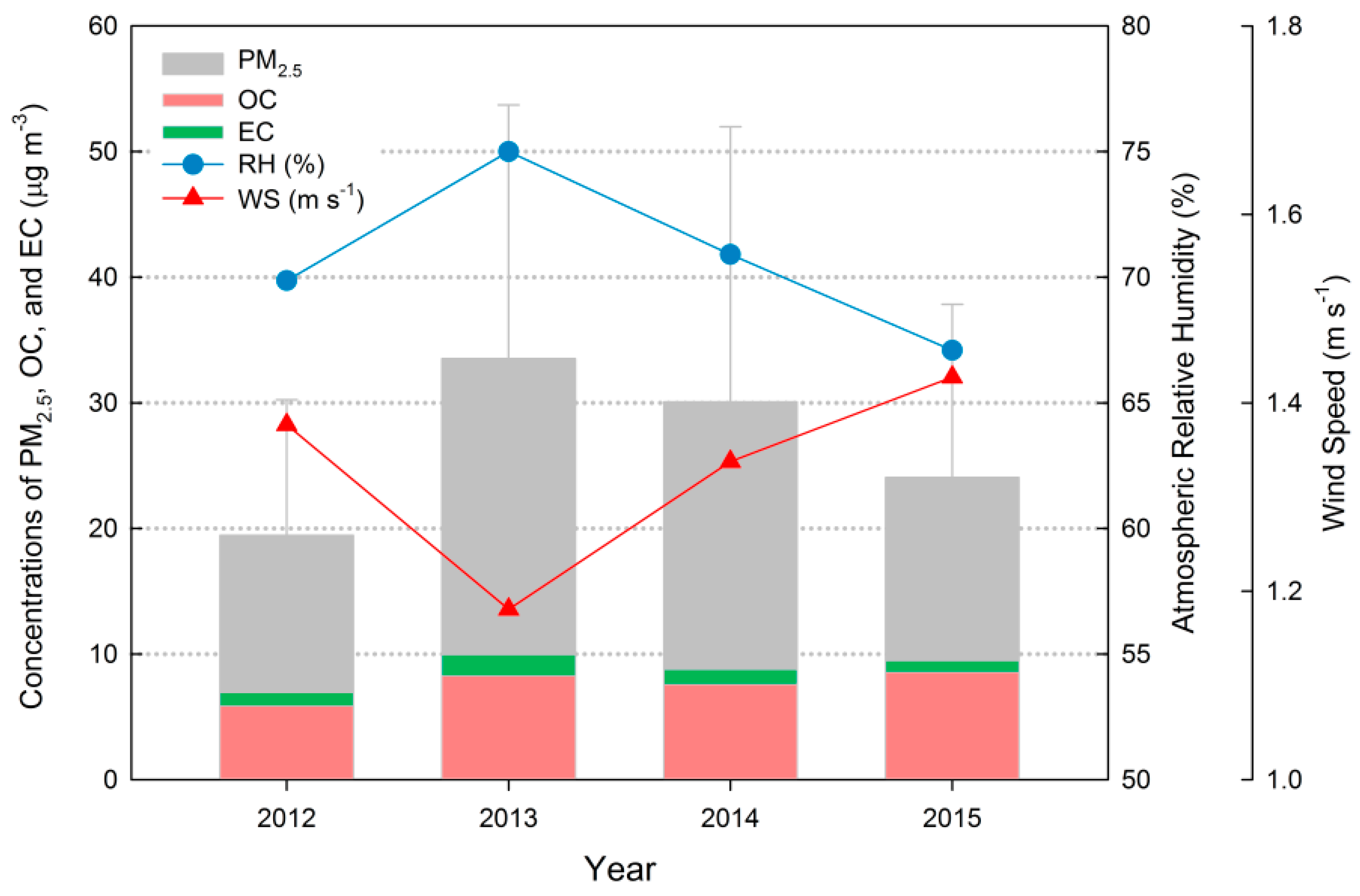
In this study, 363 samples of PM2.5 were collected throughout the whole sampling period. The average PM2.5 concentration was 27.8 ± 18.8 μg m−3, which exceeds the annual NAAQS of Korea of 25 μg m−3 (Note that the annual PM2.5 NAAQS has been strengthened to 15 μg m−3 in 2018). Seasonal PM2.5 concentrations showed the highest value in the winter (40.5 ± 22.1 μg m−3) and the lowest value in the summer (16.9 ± 11.1 μg m−3) (Table 3, ANOVA test, p-value < 0.001), which is frequently observed in other studies in Korea [14]. The percentage of the samples exceeding the daily NAAQS of Korea of 50 μg m−3 (Note that the daily NAAQS has been strengthened to 35 μg m−3 in 2018) was 10.2% (N = 37). Most of the high concentration events (>50 μg m−3) occurred in the spring (N = 10) and winter (N = 25) while the average PM2.5 concentration was 68.0 ± 16.1 μg m−3. Among 37 high concentration events, 7 fog events and 25 mist events occurred, which indicates that a high content of water vapor and low wind speed characterized environmental conditions that were conducive to PM2.5 accumulation. Previous studies showed that the humidity significantly affected the secondary organic aerosols especially those formed by aromatic volatile hydrocarbons [22,23] as well as the secondary inorganic aerosols such as (NH4)2SO4 and NH4NO3 [24]. There are many large artificial reservoirs in this city frequently causing fogs, which may be an important factor leading to the high PM2.5 concentration in this city despite the low PM2.5 emissions compared with other cities. Yearly average PM2.5 concentration was the highest in 2013. This also coincided with the highest relative humidity and the lowest average wind speed (Figure 2).
Some previous research has suggested that PM2.5 concentration is affected by meteorological factors including temperature, wind speed, and relative humidity (RH) [25,26]. There were statistical correlations between PM2.5 and temperature, wind speed, and RH at a significance level of 0.05 (Pearson R = −0.431, p-value < 0.001 for temperature, R = −0.364, p-value < 0.001 for wind speed, R = 0.118, p-value = 0.029). When the data were limited to winter only, the effect of RH on PM2.5 was more evident, which showed a Pearson R of 0.478 (p-value < 0.001). There was no correlation between PM2.5 and temperature. We found a statistical significant multiple linear relationship between PM2.5 with RH and wind speed in the winter.
where RH and WS indicate the atmospheric relative humidity (%) and wind speed (m s−1), respectively. The multiple linear equation fits the data well (R2 = 0.261, R = 0.511, p-value < 0.001) and both variables of RH and WS and constant were statistically significant (p-value < 0.001). When each of the RH and WS was used as a single independent variable, the PM2.5 regression equation was still significant with a Pearson correlation coefficient of 0.478 (R2 = 0.228, p-value < 0.001) for RH and0.439 (R2 = 0.193, p-value < 0.001), which was somewhat lower than that of the multiple regression. This result indicates that the RH can play a significant role on the high PM2.5 concentration often observed during winter at this site. Significant correlation between PM2.5 and RH was not observed during any other season.
PM2.5 = 0.52 RH − 8.36 WS + 11.84
The average OC and EC concentrations were 7.8 ± 4.6 μg m−3 and 1.2 ± 0.9 μg m−3, which contribute 27.9% and 4.4% of the PM2.5 mass, respectively (Table 3). Both the OC and EC concentrations were the highest in the winter (OC = 10.7 ± 5.4 μg m−3, EC = 1.8 ± 1.3 μg m−3) and the lowest in the summer (OC = 5.6 ± 3.0 μg m−3, EC = 0.7 ± 0.3 μg m−3) (Table 3, ANOVA test, p-value < 0.001). However, the OC contribution to PM2.5 mass was the highest in the summer (33.5%) while the EC contribution was the highest in the fall (5.5%) (Table 3). Over the whole sampling period, the average OC/EC ratio was 7.7, which was considerably higher than those measured in other major cities in Korea (Table 4). In addition, the fraction of OC in total PM2.5 was also markedly higher at this site at approximately 28% while those in other sites ranged from 10% to 22%.
These results indicate that secondary OC was important and/or primary OC emitted by sources besides vehicular emission was predominant. Previous studies have stated OC/EC ratios of 1.0 to 4.2 for diesel-vehicle and gasoline-vehicle exhaust [37,38], from 2.5 to 10.5 for residential coal smoke [39], from 16.8 to 40 for wood combustion [40], from 32.9 to 81.6 for kitchen emissions [41], and approximately 7.7 for biomass burning [37,40]. The seasonally averaged OC/EC ratios were 7.6, 10.0, 5.9, and 6.8 for spring, summer, fall, and winter in this study while the high OC/EC ratio in the summer was thought to be due to active photochemical reactions.
PC was predominant at this site and contributed 17%–50% (31.1% on average) of total OC. There was a distinct seasonal variation for PC, which was typically higher in the winter and the spring and lower in the summer (Figure 3). A previous study found that the PC concentration was enhanced during the harvest season and smoke events [42], which indicates a possible relation with biomass burning. The second-most contributor to OC was OC1 and its fraction of total OC showed a contrasting seasonal trend, which exhibited a high contribution in the summertime (Figure 3). Therefore, the organic carbons with low molecular weight were predominantly formed secondarily via photochemical reactions. A few previous studies [43,44,45] suggested that primary OC1 and OC2 were mainly emitted from the combustion of solid fuels such as biomass and coal while OC3 and OC4 were predominantly emitted from the combustion of gasoline and diesel or from road dust. In this study, the concentration of OC1 + OC2 surpassed OC3 + OC4 (Figure 3), which possibly indicates that biomass and/or coal burning was more important than vehicular emissions in terms of the primary OC concentration.
3.2. Primary Organic Carbon (POC) and Secondary Organic Carbon (SOC)
Secondary organic carbon (SOC) was estimated by using the following equations as Turpin and Huntzicker (1995) [46] suggested.
where OCpri, OCsec, and OCtot represent the concentrations of primary OC, secondary OC, and total OC, respectively. In Equation (2), a is the OC concentration emitted from non-combustion sources, which has often been negligible in previous studies [46]. (OC/EC)pri indicates the OC/EC ratio directly emitted from combustion sources, which has often been estimated from the minimum OC/EC ratio [2]. In this study, Deming regression was used to estimate the a and the (OC/EC)pri of the samples with the lowest 10% of the OC/EC ratio values for each season, which was used in the studies of Chu (2005) and Saylor et al. (2006) [47,48]. The Deming regression equations derived for each season are shown in Table 5 (and Figure S1), which indicated that the (OC/EC)pri ranged from 3.2 to 4.7 and that the POC from non-combustion sources was estimated to be negligible due to being <0.2 μg m−3 for all seasons.
Throughout the sampling period, the average POC and SOC concentrations were 4.7 ± 3.3 μg m−3 and 3.4 ± 2.7 μg m−3, respectively (Table 3). SOC contributed approximately 42% of total OC throughout the sampling period, which increased to 51% in the summer time. This suggests that SOC was being actively formed via photochemical reactions. Although the SOC fraction in the summertime was considerably higher than those during other seasons, it was relatively lower than those observed in other cities and ranged from 53% to 63% [28,31,49]. This indicated that the contribution from primary combustion sources was also important throughout the season.
Among all of the OC fractions, the best correlation with POC was found with PC (Pearson R = 0.78) while the highest correlation coefficient for SOC was observed with OC1 (Pearson R = 0.67), which indicated that a predominant fraction of PC was directly emitted from combustion sources and that a significant portion of the semi-volatile organic carbon such as OC1 was formed secondarily by reactions in the ambient air.
3.3. Water-Soluble Organic Carbon
Average WSOC concentration was 4.0 ± 1.8 μg m−3 and contributed approximately 51.1% of OC. WSOC showed the highest concentration in the winter (5.0 ± 1.5 μg m−3) and the lowest concentration in the summer (2.4 ± 0.8 μg m−3) (Figure 4). The WSOC fraction of OC was also lower in the summer (36%) than during other seasons (57%). Although a few previous studies suggested that WSOC is strongly related to SOC [50,51], the correlation coefficient of WSOC was lower with SOC (R = 0.17) than with POC (R = 0.49, p-value < 0.0001) in this study. On the other hand, PC showed a good correlation with POC and was also significantly correlated with WSOC (R = 0.70, p-value < 0.0001), which indicated that WSOC was not likely to be formed secondarily in ambient air but was probably directly emitted from combustion sources such as biomass burning.
3.4. Polycyclic Aromatic Hydrocarbons
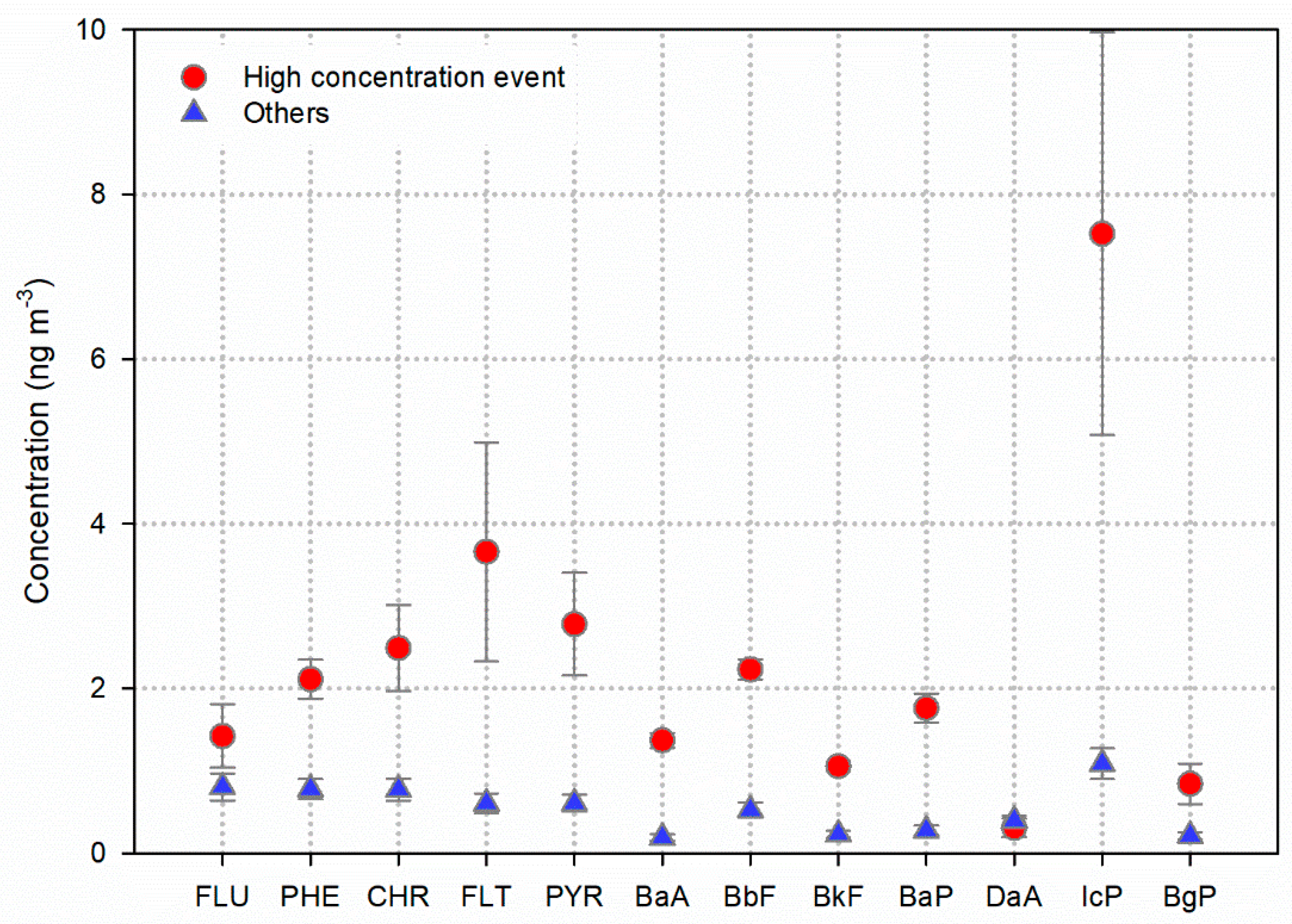
∑PAHs concentrations were significantly higher in the winter than in other seasons because PAHs are mainly emitted from incomplete combustion and are also semi-volatile compounds. Since PAHs are semi-volatile, their concentrations were high in the winter and low in the summer. Low molecular weight (LMW) PAHs with two or three rings are likely to exist as gases due to their high vapor pressure and result in low concentrations in particulate matter (Table 6). On the other hand, high molecular weight (HMW) PAHs with five or six rings tend to exist in the particulate phase due to their low vapor pressure and they are predominant in the atmosphere. ∑PAHs were positively correlated with EC (r = 0.74, p-value < 0.001) and PM2.5 (r = 0.66, p-value < 0.001) while the correlation with OC was not statistically significant (r = 0.33, p-value = 0.051). According to Di Wu et al. (2014) [52], carcinogenic PAHs (C-PAHs) include BaA, BbF, BkF, BaP, DaA, and IcP. Although the summed concentration of carcinogenic PAHs was significantly higher in the winter (8.7 ± 5.4 ng m−3) than in the spring (2.7 ± 2.5 ng m−3) or summer (1.0 ± 0.6 ng m−3), its fraction in ∑PAHs was 46.1%, 57.0%, and 66.4% in the winter, the spring, and the summer, respectively. This indicates that the toxicity per PAHs mass was the highest in the summer. The main PAH species emitted from combustion sources include FLT, PYR, CHR, BbF, BkF, BaA, BaP, IcP, and BgP [53] and their summed concentration was 15.6 ± 7.7 ng m−3 in the winter, which contributed 82.7% of ∑PAHs and 0.7 ± 0.5 ng m−3 in the summer. This adds 49% of ∑PAHs. The top 10% of ∑PAHs samples showed 27.6 ± 6.8 μg m−3 on average and mostly occurred in January. Compared with other samples, most PAH species showed significantly higher concentrations for the top 10% of ∑PAHs samples. The highest increase was observed for FLT followed by IcP, but FLU, DaA, and BgP did not increase for the top 10% of ∑PAHs samples (Figure 5). IcP and FLT are mainly emitted from the combustion of solid fuels such as coal and biomass [54,55] rather than petrogenic and pyrogenic sources, which shows that coal and/or biomass combustion greatly enhanced the concentrations of ∑PAHs.
4. Source Identification
Both the fraction and concentration of organic carbon are quite high at this site compared with those observed in other cities in Korea (Table 4). The OC/EC ratio was, therefore, also high, reaching 7.7 on average. In order to identify the reason for the high OC/EC ratio, the top 10% of the OC/EC ratio samples were selected. The average POC and SOC concentrations were 2.2 ± 1.3 and 5.8 ± 3.3 μg m−3 and showed a much higher SOC fraction (72.9%) than over the whole sampling period (43.1%) because 69% of the top 10% of OC/EC samples were taken in the summer. Most notably, the correlation between POC and SOC was very good (r = 0.89, p-value < 0.001) for the top 10% OC/EC ratio. In general, POC is not expected to have a good correlation with SOC because the sources and formation pathways are different for POC and SOC, which was also shown in this study over the whole sampling period (r = 0.19). The high correlation between POC and SOC may suggest that the POC and precursors of SOC were emitted from the same sources. However, POC is mainly emitted from combustion sources while volatile organic compounds (VOCs), which is the precursor of SOC, are mainly emitted from the usage of organic solvents (75% of the total VOC emissions in this city). Approximately 17% of VOCs are also emitted from biomass burning, which is a major possible contributor to POC. This suggests one explanation for the high OC/EC ratio. Another plausible reason for the high correlation between POC and SOC is that the precursors of SOC and POC were emitted in industrial and urban areas (such as Seoul and Incheon in Figure 1) and SOC may have formed during regional or long-range transport, which leads to a good correlation between POC and SOC at this site.
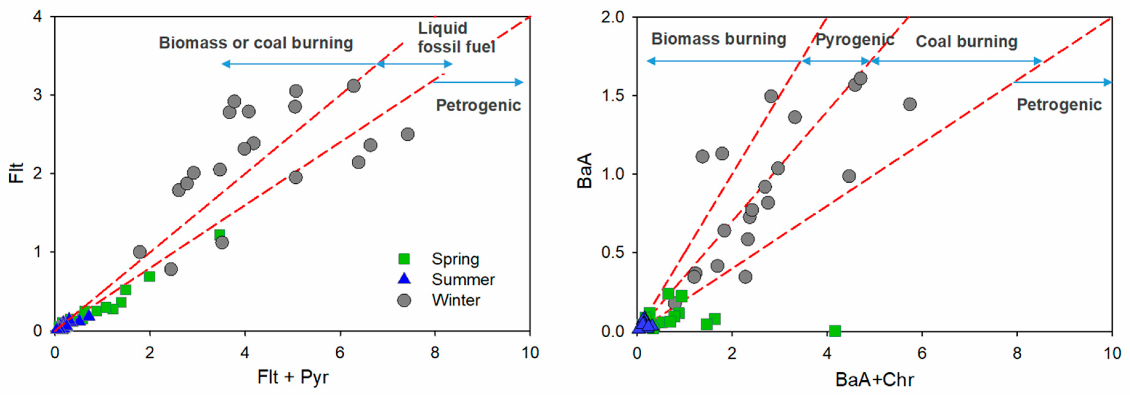
Dachs et al., (2002) [56] reported that the major sources of LMW PAHs with two or three rings, MMW PAHs with four rings, and HMW PAHs with five or six rings are pyrolytic processes due to incomplete combustion of fossil fuels, coal, or biomass combustion and vehicular emissions, respectively. In this study, the fraction of MMW PAHs in ∑PAHs was the highest in the winter and the lowest in the summer, which indicates that coal and biomass combustion were important sources for PAHs in the winter but were not significant in the summer (Table 6). On the other hand, the fraction of HMW PAHs, which is the indicator of the relative contribution of vehicular sources, increased in the summer as the effects of coal or biomass combustion on PAHs declined (Table 6). To identify the major sources affecting PAHs, diagnostic ratios are often used [57]. Flt/(Flt + Pyr) ratio is less than 0.4 for petrogenic sources in between 0.4 and 0.5 for liquid fossil fuel combustion and larger than 0.5 for biomass or coal combustion [58,59]. In this study, most of the Flt/(Flt + Pyr) ratios in the spring and summer were less than 0.4, which indicates the importance of petrogenic sources, while biomass and coal burning were shown to be predominant in the winter (Figure 6). The seasonal average Flt/(Flt + Pyr) ratios were 0.56 for winter, 0.40 for the spring, and 0.33 for the summer. BaA/(BaA + Chr) is also used to identify the source type. BaA/(BaA + Chr) of less than 0.2 indicates a petrogenic source while it generally ranges from 0.2 to 0.35 for coal burning. If BaA/(BaA + Chr) is larger than 0.35, the pyrogenic sources including incomplete combustion of petroleum and vehicular emissions are important and it is larger than 0.5 for biomass combustion. In this study, different BaA/(BaA + Chr) ratios occurred in different seasons with the average BaA/(BaA + Chr) being 0.35, 0.19, and 0.34 for the winter, the spring, and the summer, respectively. In the spring, BaA/(BaA + Chr) ratios were generally less than 0.2 (Figure 6), which indicated petrogenic sources. This was consistent with the result of BaA/(BaA + Chr). In the summer, the BaA/(BaA + Chr) ratios indicate that petrogenic and pyrogenic sources were important while coal and biomass burning were not significant. On the other hand, the BaA/(BaA + Chr) ratios encompassed a wide range of coal burning, pyrogenic sources, and biomass burning in the winter (Figure 6). The ratio of IcP/(IcP + BgP) has been used to identify the effect of vehicular emissions vs. coal and biomass combustion and most of the IcP/(IcP + BgP) ratios were larger than 0.5, which indicates the major effect of coal and biomass burning in this study.
5. Conclusions
In this study, PM2.5 and its carbonaceous compounds including OC, EC, WSOC, and PAHs were measured over more than three years. The average PM2.5 concentration exceeded the annual NAAQS and high PM2.5 was often observed concomitantly with high relative humidity and low wind speed. Both OC and the OC/PM2.5 fraction were considerably higher than those measured in other cities in Korea. Considering the relatively low OC/EC ratio for vehicle exhaust, the high OC concentration should be explained by some other sources. When confined to the top 10% of OC/EC ratio samples, POC was highly correlated with SOC even though the main sources of POC and the precursors of SOC are different. This result suggests that the precursors of SOC and POC were emitted in industrial and urban areas and SOC was produced while they were being transported to this city. Although the top 10% of high OC/EC ratio samples could be explained by SOC formation during regional or long-range transport, combustion was likely to account for the high OC concentrations that consistently occurred throughout the whole sampling period. WSOC, which might be related to SOC or biomass burning according to previous studies, was significantly correlated with POC but not SOC in this study, which indicates that WSOC was emitted from biomass burning. Using diagnostic ratios of PAHs, biomass and/or coal burning were also shown to be the predominant sources in the winter. It should be noted that the source assignment based on a single ratio can be misleading because of gas-particle partitioning and deposition during transport. It should also be noted that the seasonality of PAHs was only valid for the duration of the sampling carried out in this study, which included one spring, one summer, and one winter.
Supplementary Materials
The following are available online at https://www.mdpi.com/2073-4433/9/12/490/s1, Figure S1: Deming regression analysis of organic carbon (OC) and elemental carbon (EC) in each season.
Author Contributions
The work presented in this case was carried out in collaboration between all authors. J.-M.P. analyzed the data and wrote the paper. S.-H.C. and H.-W.K. performed the experiments and interpreted the results. Y.-J.H. defined the research theme, interpreted the results, and wrote the paper.
Funding
This research was funded by a grant from the Ministry of Environment, Republic of Korea, and by a grant from the National Research Foundation of Korea (NRF_2017K1A3A1A12073373).
Conflicts of Interest
The authors declare no conflict of interest. The funders had no role in the design of the study, in the collection, analyses, or interpretation of data, in the writing of the manuscript, or in the decision to publish the results.
References
- Joint, W.; World Health Organization. Health Risks of Particulate Matter from Long-Range Transboundary Air Pollution; WHO Regional Office for Europe: Copenhagen, Denmark, 2006. [Google Scholar]
- Grivas, G.; Cheristanidis, S.; Chaloulakou, A. Elemental and organic carbon in the urban environment of Athens. Seasonal and diurnal variations and estimates of secondary organic carbon. Sci. Total Environ. 2012, 414, 535–545. [Google Scholar] [CrossRef] [PubMed]
- Kondo, Y.; Miyazaki, Y.; Takegawa, N.; Miyakawa, T.; Weber, R.; Jimenez, J.L.; Zhang, Q.; Worsnop, D. Oxygenated and water-soluble organic aerosols in Tokyo. J. Geophys. Res. Atmos. 2007, 112. [Google Scholar] [CrossRef] [Green Version]
- Miyazaki, Y.; Kondo, Y.; Takegawa, N.; Komazaki, Y.; Fukuda, M.; Kawamura, K.; Mochida, M.; Okuzawa, K.; Weber, R.J. Time-resolved measurements of water-soluble organic carbon in Tokyo. J. Geophys. Res. Atmos. 2006, 111. [Google Scholar] [CrossRef] [Green Version]
- Sullivan, A.P.; Weber, R.J. Chemical characterization of the ambient organic aerosol soluble in water: 2. Isolation of acid, neutral, and basic fractions by modified size-exclusion chromatography. J. Geophys. Res. Atmos. 2006, 111. [Google Scholar] [CrossRef] [Green Version]
- Yan, B.; Zheng, M.; Hu, Y.; Ding, X.; Sullivan, A.P.; Weber, R.J.; Baek, J.; Edgerton, E.S.; Russell, A.G. Roadside, urban, and rural comparison of primary and secondary organic molecular markers in ambient PM2.5. Environ. Sci. Technol. 2009, 43, 4287–4293. [Google Scholar] [CrossRef]
- Weber, R.J.; Sullivan, A.P.; Peltier, R.E.; Russell, A.; Yan, B.; Zheng, M.; De Gouw, J.; Warneke, C.; Brock, C.; Holloway, J.S. A study of secondary organic aerosol formation in the anthropogenic-influenced southeastern United States. J. Geophys. Res. Atmos. 2007, 112. [Google Scholar] [CrossRef] [Green Version]
- Hecobian, A.; Zhang, X.; Zheng, M.; Frank, N.; Edgerton, E.S.; Weber, R.J. Water-Soluble Organic Aerosol material and the light-absorption characteristics of aqueous extracts measured over the Southeastern United States. Atmos. Chem. Phys. 2010, 10, 5965–5977. [Google Scholar] [CrossRef]
- Pathak, R.K.; Wang, T.; Ho, K.; Lee, S. Characteristics of summertime PM2.5 organic and elemental carbon in four major Chinese cities: Implications of high acidity for water-soluble organic carbon (WSOC). Atmos. Environ. 2011, 45, 318–325. [Google Scholar] [CrossRef]
- Afroz, R.; Hassan, M.N.; Ibrahim, N.A. Review of air pollution and health impacts in Malaysia. Environ. Res. 2003, 92, 71–77. [Google Scholar] [CrossRef]
- Fang, G.; Huang, J.; Huang, Y. Polycyclic Aromatic Hydrocarbon Pollutants in the Asian Atmosphere During 2001 to 2009. Environ. Forensics 2010, 11, 207–215. [Google Scholar] [CrossRef]
- International Agency for Research on Cancer (IARC). Agents Classified by the IARC Monographs; International Agency for Research on Cancer, World Health Organization: Lyon, France, 6937; Volumes 1–109. [Google Scholar]
- Cheng, Z.; Luo, L.; Wang, S.; Wang, Y.; Sharma, S.; Shimadera, H.; Wang, X.; Bressi, M.; de Miranda, R.M.; Jiang, J. Status and characteristics of ambient PM2.5 pollution in global megacities. Environ. Int. 2016, 89, 212–221. [Google Scholar] [CrossRef] [PubMed]
- Han, Y.; Kim, H.; Cho, S.; Kim, P.; Kim, W. Metallic elements in PM2.5 in different functional areas of Korea: Concentrations and source identification. Atmos. Res. 2015, 153, 416–428. [Google Scholar] [CrossRef]
- Vellingiri, K.; Kim, K.; Ma, C.; Kang, C.; Lee, J.; Kim, I.; Brown, R.J. Ambient particulate matter in a central urban area of Seoul, Korea. Chemosphere 2015, 119, 812–819. [Google Scholar] [CrossRef] [PubMed]
- Jeong, J.I.; Park, R.J.; Woo, J.; Han, Y.; Yi, S. Source contributions to carbonaceous aerosol concentrations in Korea. Atmos. Environ. 2011, 45, 1116–1125. [Google Scholar] [CrossRef]
- Matter, P. Speciation Guidance (Final Draft); US Environmental Protection Agency: Research Triangle Park, NC, USA, 1999.
- Birch, M.E.; Cary, R.A. Elemental Carbon-Based Method for Monitoring Occupational Exposures to Particulate Diesel Exhaust. Aerosol Sci. Technol. 1996, 25, 221–241. [Google Scholar] [CrossRef] [Green Version]
- Health Division of Physical Sciences NIOSH. Manual of Analytical Methods; US Department of Health and Human Services, Public Health Service, Centers for Disease Control and Prevention, National Institute for Occupational Safety and Health, Division of Physical Sciences and Engineering: Atlanta, GA, USA, 1994.
- US EPA. Method 8100 Polynuclear Aromatic Hydrocarbons; US EPA: Washington, DC, USA, 1986; pp. 1–10.
- Ott, W.R. Environmental Statistics and data Analysis; CRC Press: Boca Raton, FL, USA, 1995. [Google Scholar]
- Hu, D.; Jiang, J. PM2.5 pollution and risk for lung cancer: A rising issue in China. J. Environ. Prot. 2014, 5, 731. [Google Scholar] [CrossRef]
- Kamens, R.M.; Zhang, H.; Chen, E.H.; Zhou, Y.; Parikh, H.M.; Wilson, R.L.; Galloway, K.E.; Rosen, E.P. Secondary organic aerosol formation from toluene in an atmospheric hydrocarbon mixture: Water and particle seed effects. Atmos. Environ. 2011, 45, 2324–2334. [Google Scholar] [CrossRef]
- Jung, J.-H.; Han, Y.-J. Study on Characteristics of PM2.5 and Its Ionic Constituents in Chuncheon, Korea. J. Korean Soc. Atmos. Environ. 2008, 24, 682–692. [Google Scholar] [CrossRef]
- Kozáková, J.; Pokorná, P.; Černíková, A.; Hovorka, J.; Braniš, M.; Moravec, P.; Schwarz, J. The association between intermodal (PM1–2.5) and PM1, PM2.5, coarse fraction and meteorological parameters in various environments in Central Europe. Aerosol Air Qual. Res. 2017, 17, 1234–1243. [Google Scholar] [CrossRef]
- Kozáková, J.; Leoni, C.; Klán, M.; Hovorka, J.; Racek, M.; Koštejn, M.; Ondráček, J.; Moravec, P.; Schwarz, J. Chemical Characterization of PM1–2.5 and its Associations with PM1, PM2.5–10 and Meteorology in Urban and Suburban Environments. Aerosol Air Qual. Res. 2018, 18, 1684–1697. [Google Scholar] [CrossRef]
- Jeon, H.; Park, J.; Kim, H.; Sung, M.; Choi, J.; Hong, Y.; Hong, J. The characteristics of PM2.5 concentration and chemical composition of Seoul metropolitan and inflow background area in Korea peninsula. J. Korean Soc. Urban Environ. 2015, 15, 261–271. [Google Scholar]
- Choi, J.; Heo, J.; Ban, S.; Yi, S.; Zoh, K. Chemical characteristics of PM2.5 aerosol in Incheon, Korea. Atmos. Environ. 2012, 60, 583–592. [Google Scholar] [CrossRef]
- Park, S.S.; Cho, S.Y.; Kim, S.J. Chemical Characteristics of Water Soluble Components in Fine Particulate Matter at a Gwangju area. Korean Chem. Eng. Res. 2010, 48, 20–26. [Google Scholar]
- Han, J.; Kim, J.; Kang, E.; Lee, M.; Shim, J. Ionic Compositions and Carbonaceous Matter of PM2.5 at Ieodo Ocean Research Station. J. Korean Soc. Atmos. Environ. 2013, 29, 701–712. [Google Scholar] [CrossRef]
- Kim, H.; Jung, J.; Lee, J.; Lee, S. Seasonal Characteristics of Organic Carbon and Elemental Carbon in PM2.5 in Daejeon. J. Korean Soc. Atmos. Environ. 2015, 31, 28–40. [Google Scholar] [CrossRef]
- Kang, B.W.; Lee, H.S. Source Apportionment of Fine Particulate Matter (PM2.5) in the Chungju City. J. Korean Soc. Atmos. Environ. 2015, 31, 437–448. [Google Scholar] [CrossRef]
- Li, K.C.; Hwang, I. Characteristics of PM2.5 in Gyeongsan Using Statistical Analysis. J. Korean Soc. Atmos. Environ. 2015, 31, 520–529. [Google Scholar] [CrossRef]
- Paraskevopoulou, D.; Liakakou, E.; Gerasopoulos, E.; Theodosi, C.; Mihalopoulos, N. Long-term characterization of organic and elemental carbon in the PM2.5 fraction: The case of Athens, Greece. Atmos. Chem. Phys. 2014, 14, 13313–13325. [Google Scholar] [CrossRef]
- Plaza, J.; Artíñano, B.; Salvador, P.; Gómez-Moreno, F.J.; Pujadas, M.; Pio, C.A. Short-term secondary organic carbon estimations with a modified OC/EC primary ratio method at a suburban site in Madrid (Spain). Atmos. Environ. 2011, 45, 2496–2506. [Google Scholar] [CrossRef]
- Zhang, R.; Tao, J.; Ho, K.; Shen, Z.; Wang, G.; Cao, J.; Liu, S.; Zhang, L.; Lee, S. Characterization of atmospheric organic and elemental carbon of PM2.5 in a typical semi-arid area of Northeastern China. Aerosol Air Qual. Res. 2012, 12, 792–802. [Google Scholar] [CrossRef]
- Schauer, J.J.; Kleeman, M.J.; Cass, G.R.; Simoneit, B.R. Measurement of emissions from air pollution sources. 2. C1 through C30 organic compounds from medium duty diesel trucks. Environ. Sci. Technol. 1999, 33, 1578–1587. [Google Scholar] [CrossRef]
- Schauer, J.J.; Kleeman, M.J.; Cass, G.R.; Simoneit, B.R. Measurement of emissions from air pollution sources. 5. C1−C32 organic compounds from gasoline-powered motor vehicles. Environ. Sci. Technol. 2002, 36, 1169–1180. [Google Scholar] [CrossRef] [PubMed]
- Chen, Y.; Zhi, G.; Feng, Y.; Fu, J.; Feng, J.; Sheng, G.; Simoneit, B.R. Measurements of emission factors for primary carbonaceous particles from residential raw-coal combustion in China. Geophys. Res. Lett. 2006, 33. [Google Scholar] [CrossRef] [Green Version]
- Schauer, J.J.; Kleeman, M.J.; Cass, G.R.; Simoneit, B.R. Measurement of emissions from air pollution sources. 3. C1−C29 organic compounds from fireplace combustion of wood. Environ. Sci. Technol. 2001, 35, 1716–1728. [Google Scholar] [CrossRef] [PubMed]
- He, L.; Hu, M.; Huang, X.; Yu, B.; Zhang, Y.; Liu, D. Measurement of emissions of fine particulate organic matter from Chinese cooking. Atmos. Environ. 2004, 38, 6557–6564. [Google Scholar] [CrossRef]
- Gu, J.; Bai, Z.; Liu, A.; Wu, L.; Xie, Y.; Li, W.; Dong, H.; Zhang, X. Characterization of atmospheric organic carbon and element carbon of PM2.5 and PM10 at Tianjin, China. Aerosol Air Qual. Res. 2010, 10, 167–176. [Google Scholar] [CrossRef]
- Chow, J.C.; Watson, J.G.; Kuhns, H.; Etyemezian, V.; Lowenthal, D.H.; Crow, D.; Kohl, S.D.; Engelbrecht, J.P.; Green, M.C. Source profiles for industrial, mobile, and area sources in the Big Bend Regional Aerosol Visibility and Observational study. Chemosphere 2004, 54, 185–208. [Google Scholar] [CrossRef] [PubMed]
- Grabowsky, J.; Streibel, T.; Sklorz, M.; Chow, J.C.; Watson, J.G.; Mamakos, A.; Zimmermann, R. Hyphenation of a carbon analyzer to photo-ionization mass spectrometry to unravel the organic composition of particulate matter on a molecular level. Anal. Bioanal. Chem. 2011, 401, 3153–3164. [Google Scholar] [CrossRef]
- Cao, J.; Huang, H.; Lee, S.; Chow, J.C.; Zou, C.; Ho, K.; Watson, J.G. Indoor/outdoor relationships for organic and elemental carbon in PM2.5 at residential homes in Guangzhou, China. Aerosol Air Qual. Res. 2012, 12, 902–910. [Google Scholar] [CrossRef]
- Turpin, B.J.; Huntzicker, J.J. Identification of secondary organic aerosol episodes and quantitation of primary and secondary organic aerosol concentrations during SCAQS. Atmos. Environ. 1995, 29, 3527–3544. [Google Scholar] [CrossRef]
- Chu, S. Stable estimate of primary OC/EC ratios in the EC tracer method. Atmos. Environ. 2005, 39, 1383–1392. [Google Scholar] [CrossRef]
- Saylor, R.D.; Edgerton, E.S.; Hartsell, B.E. Linear regression techniques for use in the EC tracer method of secondary organic aerosol estimation. Atmos. Environ. 2006, 40, 7546–7556. [Google Scholar] [CrossRef]
- Na, K.; Sawant, A.; Song, C.; Cocker, D., III. Primary and secondary carbonaceous species in the atmosphere of Western Riverside County, California. Atmos. Environ. 2004, 38, 1345–1355. [Google Scholar]
- Claeys, M.; Graham, B.; Vas, G.; Wang, W.; Vermeylen, R.; Pashynska, V.; Cafmeyer, J.; Guyon, P.; Andreae, M.O.; Artaxo, P.; et al. Formation of secondary organic aerosols through photooxidation of isoprene. Science 2004, 303, 1173–1176. [Google Scholar] [CrossRef]
- Schichtel, B.A.; Malm, W.C.; Bench, G.; Fallon, S.; McDade, C.E.; Chow, J.C.; Watson, J.G. Fossil and contemporary fine particulate carbon fractions at 12 rural and urban sites in the United States. J. Geophys. Res. Atmos. 2008, 113. [Google Scholar] [CrossRef] [Green Version]
- Wu, D.; Wang, Z.; Chen, J.; Kong, S.; Fu, X.; Deng, H.; Shao, G.; Wu, G. Polycyclic aromatic hydrocarbons (PAHs) in atmospheric PM2.5 and PM10 at a coal-based industrial city: Implication for PAH control at industrial agglomeration regions, China. Atmos. Res. 2014, 149, 217–229. [Google Scholar] [CrossRef]
- Kong, S.; Ding, X.; Bai, Z.; Han, B.; Chen, L.; Shi, J.; Li, Z. A seasonal study of polycyclic aromatic hydrocarbons (PAHs) in PM2.5 and PM2.5-10 in five typical cities of Liaoning Province, China. J. Hazard. Mater. 2010, 183, 70–80. [Google Scholar] [CrossRef] [PubMed]
- Lee, J.Y.; Kim, Y.P.; Kang, C.; Ghim, Y.S.; Kaneyasu, N. Temporal trend and long-range transport of particulate polycyclic aromatic hydrocarbons at Gosan in northeast Asia between 2001 and 2004. J. Geophys. Res. Atmos. 2006, 111. [Google Scholar] [CrossRef] [Green Version]
- Liu, Y.; Yu, Y.; Liu, M.; Lu, M.; Ge, R.; Li, S.; Liu, X.; Dong, W.; Qadeer, A. Characterization and source identification of PM2.5-bound polycyclic aromatic hydrocarbons (PAHs) in different seasons from Shanghai, China. Sci. Total Environ. 2018, 644, 725–735. [Google Scholar] [CrossRef]
- Dachs, J.; Glenn IV, T.R.; Gigliotti, C.L.; Brunciak, P.; Totten, L.A.; Nelson, E.D.; Franz, T.P.; Eisenreich, S.J. Processes driving the short-term variability of polycyclic aromatic hydrocarbons in the Baltimore and northern Chesapeake Bay atmosphere, USA. Atmos. Environ. 2002, 36, 2281–2295. [Google Scholar] [CrossRef]
- Khan, M.F.; Latif, M.T.; Lim, C.H.; Amil, N.; Jaafar, S.A.; Dominick, D.; Nadzir, M.S.M.; Sahani, M.; Tahir, N.M. Seasonal effect and source apportionment of polycyclic aromatic hydrocarbons in PM2.5. Atmos. Environ. 2015, 106, 178–190. [Google Scholar] [CrossRef]
- Yunker, M.B.; Macdonald, R.W.; Vingarzan, R.; Mitchell, R.H.; Goyette, D.; Sylvestre, S. PAHs in the Fraser River basin: A critical appraisal of PAH ratios as indicators of PAH source and composition. Org. Geochem. 2002, 33, 489–515. [Google Scholar] [CrossRef]
- Roberto, J.; Lee, W.; Campos-Díaz, S.I. Soil-borne polycyclic aromatic hydrocarbons in El Paso, Texas: Analysis of a potential problem in the United States/Mexico border region. J. Hazard. Mater. 2009, 163, 946–958. [Google Scholar] [Green Version]
Figure 1.
Study area. (a) Location of South Korea. (b) The sampling site location is indicated by the black star in the red area representing the city, Chuncheon and the metropolitan region (Seoul) and major industrial regions (Incheon) are shown as green and blue areas, respectively. (c) Land cover data for the city, Chuncheon. The sampling site location is also indicated by the black star.

Figure 2.
Yearly averaged concentrations of PM2.5, OC, and EC with yearly averaged RH (relative humidity) and WS (wind speed). The error bars indicate one standard deviation.
Figure 2.
Yearly averaged concentrations of PM2.5, OC, and EC with yearly averaged RH (relative humidity) and WS (wind speed). The error bars indicate one standard deviation.

Figure 3.
Monthly averaged concentrations (left) and fractions (right) of each of the OC fragments analyzed by the NIOSH method 5040.
Figure 3.
Monthly averaged concentrations (left) and fractions (right) of each of the OC fragments analyzed by the NIOSH method 5040.

Figure 4.
Water soluble organic carbon (WSOC) concentration and WSOC/OC ratios during the whole sampling period.
Figure 4.
Water soluble organic carbon (WSOC) concentration and WSOC/OC ratios during the whole sampling period.

Figure 5.
Increment of PAH species for the top 10% of ∑PAHs samples. Note that the error bars indicate one standard error.
Figure 5.
Increment of PAH species for the top 10% of ∑PAHs samples. Note that the error bars indicate one standard error.

Figure 6.
Diagnostic ratios to identify the major sources of PAHs.


Table 1.
Experimental parameters for the thermal/optical analytical protocol.
| Gas | Hold Time (s) | Temperature (°C) | Component |
|---|---|---|---|
| He | 10 | 1 | |
| He | 80 | 310 | OC1 |
| He | 80 | 475 | OC2 |
| He | 80 | 615 | OC3 |
| He | 110 | 870 | OC4 |
| He | 45 | 550 | PC |
| O2 in He | 45 | 550 | EC1 |
| O2 in He | 45 | 625 | EC2 |
| O2 in He | 45 | 700 | EC3 |
| O2 in He | 45 | 775 | EC4 |
| O2 in He | 45 | 850 | EC5 |
| O2 in He | 110 | 870 | EC6 |
Table 2.
QA/QC results for PAH analysis. Note that RSD indicates relative standard deviation.
| Compounds | R2 | MDL (ng) | RSD (%) | Recovery (%) | Detector |
|---|---|---|---|---|---|
| FLU | 0.9985 | 0.14 | 1.9 | 78.2 | UV |
| PHE | 0.9979 | 0.11 | 6.7 | 65.9 | UV |
| CHR | 0.9994 | 0.17 | 2.9 | 76.4 | UV |
| FLT | 0.9995 | 0.08 | 1.5 | 91.8 | FLD |
| PYR | 0.9987 | 0.01 | 1.4 | 135.9 | FLD |
| BaA | 0.9990 | 0.01 | 1.1 | 109.7 | FLD |
| BbF | 0.9989 | 0.02 | 1.0 | 99.9 | FLD |
| BkF | 0.9985 | 0.01 | 0.1 | 92.3 | FLD |
| BaP | 0.9983 | 0.04 | 1.0 | 110.2 | FLD |
| DaA | 0.9991 | 0.03 | 1.2 | 106.7 | FLD |
| IcP | 0.9944 | 0.01 | 2.3 | 120.5 | FLD |
| BgP | 0.9930 | 0.00 | 2.5 | 131.5 | FLD |
Table 3.
Summarized results for PM2.5 and its carbonaceous compounds. The unit of concentration is mg m−3 and the values in parenthesis are the fractions of POC or SOC in total OC.
Table 3.
Summarized results for PM2.5 and its carbonaceous compounds. The unit of concentration is mg m−3 and the values in parenthesis are the fractions of POC or SOC in total OC.
| Period | N | PM2.5 | OC | EC | |
|---|---|---|---|---|---|
| POC | SOC | ||||
| Spring | 98 | 29.1 ± 17.5 | 4.9 ± 2.4 (64%) | 2.8 ± 1.9 (36%) | 1.1 ± 0.5 (3.9) |
| Summer | 103 | 16.9 ± 11.1 | 2.9 ± 1.3 (49%) | 3.0 ± 2.7 (51%) | 0.7 ± 0.3 (3.9) |
| Autumn | 65 | 24.5 ± 12.7 | 4.4 ± 3.3 (61%) | 2.8 ± 2.3 (39%) | 1.3 ± 1.0 (5.5) |
| Winter | 97 | 40.5 ± 22.1 | 6.1 ± 4.1 (56%) | 4.7 ± 3.3 (44%) | 1.8 ± 1.3 (4.5) |
| Total | 363 | 27.8 ± 18.8 | 4.7 ± 3.3 (58%) | 3.4 ± 2.7 (42%) | 1.2 ± 0.9 (4.4) |
Table 4.
Comparisons of measured concentrations of PM2.5 and its carbonaceous compounds with those reported in other studies. Units of PM2.5, OC, and EC are μg m−3.
Table 4.
Comparisons of measured concentrations of PM2.5 and its carbonaceous compounds with those reported in other studies. Units of PM2.5, OC, and EC are μg m−3.
| Site | Site Type | Period | PM2.5 | OC | EC | OC/EC | References |
|---|---|---|---|---|---|---|---|
| Seoul, Korea | Urban | January 2013~December 2013 | 29.5 | 4.8 | 1.8 | 2.7 | [27] |
| Incheon, Korea | Industrial | January 2009~May 2010 | 41.9 | 7.9 | 1.8 | 4.4 | [28] |
| Gwangju, Korea | Urban | December 2007~February 2008 | 27.4 | 4.5 | 1.8 | 2.7 | [29] |
| Ieodo, Korea | Rural | June 2006~June 2008 | 21.8 | 2.3 | 1.0 | 2.3 | [30] |
| Daejeon, Korea | Urban | March 2012~February 2013 | 23.6 | 5.3 | 0.8 | 6.6 | [31] |
| Chungju, Korea | Suburban | May 2013~January 2014 | 48.2 | 5.8 | 1.8 | 3.2 | [32] |
| Gyeongsan, Korea | Suburban | September 2010~December 2012 | 25.2 | 4.3 | 1.3 | 3.3 | [33] |
| Chuncheon | Suburban | April 2012~August 2015 | 27.8 | 7.8 | 1.2 | 7.7 | This study |
| Beijing, China | Urban | June~August 2005 | 68.0 | 8.2 | 4.9 | 2.2 | [9] |
| Athens, Greece | Urban | May 2008~April 2013 | 20.0 | 2.0 | 0.5 | 4.7 | [34] |
| Madrid, Spain | Urban | February 2006~June 2008 | - | 3.7 | 1.3 | 4.3 | [35] |
| Tongyu, China | Rural | April~June 2006 | - | 14.1 | 2.0 | 7.5 | [36] |
Table 5.
Deming regression equations obtained for each season.
| Season | N | Deming Regression Derived (y = bx + a) |
|---|---|---|
| Spring | 11 | y = 4.3x + 0.07 |
| Summer | 7 | y = 4.7x |
| Fall | 6 | y = 3.2x + 0.11 |
| Winter | 12 | y = 3.5x + 0.02 |
Table 6.
Seasonal variation of PAH species. Note that the percentage in parentheses indicates the fraction of LMW, MMW, or HMW PAHs in ∑PAHs.
Table 6.
Seasonal variation of PAH species. Note that the percentage in parentheses indicates the fraction of LMW, MMW, or HMW PAHs in ∑PAHs.
| Species | No. of Rings | Winter | Spring | Summer |
|---|---|---|---|---|
| PM2.5 (μg m−3) | 37.3 ± 14.7 | 23.0 ± 17.1 | 13.2 ± 8.1 | |
| 12 PAHs (ng m−3) | ||||
| FLU | 3 | 1.4 ± 1.0 | 0.2 ± 0.0 | 0.4 ± 0.3 |
| PHE | 3 | 1.6 ± 0.7 | 0.5 ± 0.4 | 0.3 ± 0.3 |
| CHR | 4 | 1.8 ± 1.0 | 0.8 ± 1.0 | 0.1 ± 0.1 |
| FLT | 4 | 2.7 ± 2.2 | 0.4 ± 0.4 | 0.1 ± 0.0 |
| PYR | 4 | 2.1 ± 1.3 | 0.6 ± 0.6 | 0.1 ± 0.1 |
| BaA | 4 | 0.9 ± 0.5 | 0.1 ± 0.1 | - |
| BbF | 5 | 1.9 ± 0.6 | 0.4 ± 0.4 | 0.1 ± 0.1 |
| BkF | 5 | 0.9 ± 0.3 | 0.2 ± 0.2 | - |
| BaP | 5 | 1.3 ± 0.6 | 0.2 ± 0.2 | 0.1 ± 0.0 |
| DaA | 5 | 0.3 ± 0.3 | 0.2 ± 0.2 | 0.6 ± 0.5 |
| IcP | 6 | 4.2 ± 4.9 | 1.8 ± 1.9 | 0.3 ± 0.3 |
| BgP | 6 | 0.8 ± 0.5 | 0.2 ± 0.2 | - |
| ∑PAHs | 19.8 ± 8.1 | 5.4 ± 3.6 | 2.1 ± 0.8 | |
| LMW PAHs | 3 | 3.0 ± 1.3 (15.2%) | 0.7 ± 0.3 (13.0%) | 0.6 ± 0.4 (28.6%) |
| MMW PAHs | 4 | 7.4 ± 3.0 (37.4%) | 1.9 ± 1.3 (35.2%) | 0.3 ± 0.2 (14.3%) |
| HMW PAHs | 5,6 | 9.3 ± 5.2 (47.0%) | 2.8 ± 2.6 (51.9%) | 1.1 ± 0.5 (52.4%) |
© 2018 by the authors. Licensee MDPI, Basel, Switzerland. This article is an open access article distributed under the terms and conditions of the Creative Commons Attribution (CC BY) license (http://creativecommons.org/licenses/by/4.0/).
Share and Cite
MDPI and ACS Style
Park, J.-M.; Han, Y.-J.; Cho, S.-H.; Kim, H.-W. Characteristics of Carbonaceous PM2.5 in a Small Residential City in Korea. Atmosphere 2018, 9, 490. https://doi.org/10.3390/atmos9120490
AMA Style
Park J-M, Han Y-J, Cho S-H, Kim H-W. Characteristics of Carbonaceous PM2.5 in a Small Residential City in Korea. Atmosphere. 2018; 9(12):490. https://doi.org/10.3390/atmos9120490
Chicago/Turabian StylePark, Jong-Min, Young-Ji Han, Sung-Hwan Cho, and Hyun-Woong Kim. 2018. "Characteristics of Carbonaceous PM2.5 in a Small Residential City in Korea" Atmosphere 9, no. 12: 490. https://doi.org/10.3390/atmos9120490
Note that from the first issue of 2016, this journal uses article numbers instead of page numbers. See further details here.