Characterizing Emissions from Agricultural Diesel Pumps in the Terai Region of Nepal

International Centre for Integrated Mountain Development (ICIMOD), G.P.O. Box 3226, Kathmandu, Nepal
*
Author to whom correspondence should be addressed.
Atmosphere 2019, 10(2), 56; https://doi.org/10.3390/atmos10020056
Submission received: 21 December 2018
/
Revised: 12 January 2019
/
Accepted: 15 January 2019
/
Published: 1 February 2019
(This article belongs to the Special Issue Air Quality in the Asia-Pacific Region)
Abstract
:Diesel irrigation pumps are a source of air pollution in the Indo-Gangetic Plain (IGP). The environmental implications of these pumps are often overlooked and very rarely addressed in the IGP. Few studies in the past have estimated the amount of diesel consumed by irrigation pumps in the IGP or other proxy variables to estimate the amount of emissions. A considerable amount of uncertainty remains in calculating emission factors (EF) using real-time measurements. We measured pollutants from nine diesel irrigation pumps in the southern ‘Terai’ belt of Nepal. Fuel-based EF were then estimated using the carbon mass balance method. The average EF for fine particulate matter (PM2.5), CO2, CO and black carbon (BC) were found to be 22.11 ± 3.71, 2218.10 ± 26.8, 275 ± 17.18 and 2.54 ± 0.71 g/L, respectively. Depending upon the pump characteristics (age, design, make, hours used, etc.) and fuel mixtures, the EF of PM2.5, BC and CO had larger inter-variability. This study provides estimates for an under-represented source of ambient air pollution which will assist in the development of better emission inventories and informed policy making.
1. Introduction
Groundwater irrigation for agricultural activities prevails in the lowland regions of the world. Previous studies report that ~38% of total cultivable lands (301 million ha) are irrigated by groundwater, globally. This is equivalent to approximately 545 km3 y−1 of consumed water use [1]. Based on the area of irrigated land, India, China and the United States of America head the list of countries using irrigation (on approximately 39, 19 and 17 million ha of land, respectively) from both surface and groundwater sources [1]. Groundwater is extracted manually or using either electricity or diesel-powered pumps [2]. In much of the developing world, diesel-powered pumps are used rather than those powered by electricity, because of the poor supply of electricity and load-shedding issues [3].
In Iran, groundwater extraction requires 2.05 billion kWh of electricity and 2 million tonnes of fuel each year [4]. In Myanmar, 77% of total irrigation is achieved by use of diesel-powered pumps [2]. In India, 2.04 million tonnes of diesel was used in 2011 for irrigation pumps [5]; in 2013, 2.98 million tonnes of diesel was used to operate irrigation pumps in Pakistan [2,6]. Across the Indo-Gangetic Plains (IGP), an estimated 10 million diesel pumps are now in operation [7,8], with a majority of pumps being operated in India, Pakistan, Bangladesh and Nepal [3,9].
Although a substantial number of diesel pumps are operational in the IGP, their environmental impact has barely been addressed [10,11]. Some of the prior research conducted in this region has focused primarily on the socio-economic aspects of groundwater extraction from the irrigation pumps [3,6,7,12]. A few of these studies discussed aspects related to the use of diesel-based irrigation pumps and its relation to food production and livelihoods of the local people. Meanwhile, the rest of them looked into the climate impacts due to greenhouse gas emissions from this particulate source [8,13]. However, there is a dearth of knowledge of the air pollution aspect related to this source. Incomplete combustion of diesel from these less efficient pumps [14] results in the emission of black carbon (BC), particulate matter (PM), CO2, CO and an array of other pollutants [15]. Previous literature has highlighted the impacts of diesel-based emissions of PM and BC on human health and the environment [16,17,18,19]. However, there is still considerable uncertainty about the quantification of emission factors (EF) from this particular source [20]. Most regional and global emission inventories include the overall emissions from the agricultural sectors, but emissions from individual sources in this sector (pumps, tractors, residual combustion and other transporting and non-transporting equipment) have not been estimated in detail. This leads to significant uncertainty about overall emissions in the region, leading to improper representation in the regional and global models [21]. In the recent past, different studies based on model simulations of the South Asian region have indicated a strong requirement for improving the existing emissions inventories by adding different under-sampled sources and updating the existing emission estimates [22,23]. To date, the available EF of different pollutants from the diesel irrigation source have mostly been determined using empirical equations based on surrogate variables such as the amount of energy required, depth of water table, age of pumps, volume of water extracted and/or area of land irrigated [6,24,25,26,27,28]. Most of these studies have focused on CO2 emissions, and do not consider pollutants such as BC or fine PM (PM2.5). To the best of our knowledge, emissions from only two diesel pumps in the IGP have been characterized recently during the NAMaSTE campaign [10,11]. There were large variations in the EF of PM2.5 and BC reported for these two pumps; this might have been due to the small sample size. A study with a large sample size and with several varieties of pumps is needed to better understand pump emissions.
The present study thus uses a bottom-up approach for estimating the fuel-based EFs of selected particulate (PM2.5 and BC) and gaseous (CO2 and CO) pollutants. This will provide robust emission estimates for inclusion in regional and global emission inventories, while also helping researchers and practitioners, and guiding policy makers in reducing the negative impacts of the diesel pumps in the region.
2. Materials and Methods
2.1. Site Description
A campaign to estimate the emissions from diesel-based irrigation pumps was conducted in Saptari, Nepal, during summer 2017. This region is located in the ‘Terai’ region and is representative of the Indo-Gangetic Plain in Nepal. This site is one of the agricultural hubs in the country that follows a three-season cropping pattern. Paddy, wheat and mustard are the major crops cultivated. Paddy production is a water-intensive agricultural practice that makes farmers dependent on different water irrigation sources. According to the Central Bureau of Statistics [29], there are a total of 30,917 water-extracting units (diesel pumps and manual pumps) in the district; these irrigate approximately 16,760 ha of agricultural land. We conducted our study of measurements from diesel irrigation pump emissions in the two wards of Surunga rural municipality in Saptari district (as shown in Figure 1). Nine agricultural diesel pumps were randomly selected in these two wards and measurements were made during the water-pumping period. The campaign was conducted during the monsoon season in 2017.
2.2. Emissions Measurement
Ratnoze1 (Mountain Air Engineering, USA) portable sampling equipment was used to measure the particulate and gaseous pollutants from the exhaust of the diesel-powered irrigation pumps. This is a customized unit designed to measure concentration of pollutants from combustion sources. More details about the Ratnoze1 equipment can be found in the publications of Mountain Air Engineering [30]. The sampler uses a dilution system (particulate-free dry air passed through two channels of silica gel) to bring exhaust emissions down within the measurable range of the sensors. Background and exhaust sensors measured the background concentrations of CO2, CO and SO2; these were used for background correction of each gas from the exhaust sample. CO2 concentrations were measured with a non-destructive infra-red (NDIR) sensor with a measurable range of 0–50000 PPM. CO and SO2 concentrations were measured with electrochemical sensors having measurable ranges of 0–5000 PPM and 0–2000 PPM, respectively. The PM sensor used the optical technique to measure the light scattering coefficient at 635 nm wavelength (a range of 0–500000 Mm−1). The sampling train of the system contained a PM2.5 size selective inlet which was then divided into four channels (Figure 2). Two channels were connected to two parallel 47 mm filter holders; these collected filter samples for laboratory analysis and to calculate PM mass concentration using the gravimetric method. The third channel was connected to a gaseous and PM sensor for measurement of real-time gaseous pollutants (CO2, CO, SO2) and PM mass-scattering coefficient. The fourth channel was connected to a MicroAeth model AE51 (AethLabs, San Francisco, CA, USA) for measuring real-time BC concentrations.
The Ratnoze1 draws the exhaust sample mixed with dilution air at a flow rate of 1500 Standard Cubic Centimeters per Minute (SCCM) at the tip of the cyclone. The flow is then distributed in channels F1 and F2 at a flow rate of 400 SCCM. A flow rate of 50 SCCM is maintained for the third channel, leading to the MicroAeth. Finally, the flow rate in the fourth channel, used to measure gaseous and particulate pollutants, is regulated in such a way that the overall flow rate is maintained at 1500 SCCM. The dilution ratio (the ratio of dilution gas by sample flow) for all measurements was maintained within the range of 4–6 to keep all parameters within the measurable range. The Ratnoze1 was kept near the exhaust pipe of the pumps when measurements were being taken (Figure 3). Each measurement cycle lasted for 60–120 min depending on the approximate PM2.5 mass deposited on the filter paper, and based on field experience. This procedure was followed in order to attain detectable levels of deposition on the filter paper. PM samples were collected on Teflo and Quartz fiber filter membranes (Pall Corporation, Hampshire, UK) of 47 mm diameter, placed in the filter holders. Strict precautions were maintained for proper handling, storage and transportation of the filter samples during and after the experiment [31]. Prior to use in the field, the Quartz filter papers were baked at 450 °C for 8 h to remove volatiles [32] and were then kept in a desiccator for 24 h to maintain their moisture conditions before measuring the initial weights. The Teflo filter membranes were also desiccated for 24 h prior to measuring initial weights. Before measuring the final weights, the filter papers and membranes were also desiccated for 24 h. The concentrations were then determined gravimetrically by subtracting the initial weights from the final weights measured by an HPBG-2285Di micro-balance (BEL Engineering, Monza (MB), ITALIA) with a resolution of 0.01 mg. To strengthen quality control measures, field blanks were also collected.
To maintain strict quality protocols, the sensors were either factory calibrated or calibrated using calibration gas mixtures immediately before sampling. The PM sensor was factory calibrated; hence, only onsite zero calibration was performed using a high-efficiency particulate air (HEPA) filter before measuring began. A factory-calibrated MicroAeth was used to measure BC. The CO gas sensors were calibrated at 0 ppm using a zero-air gas (Specialty Gases Ltd., West Bromwich, UK), and at 81 ppm using a CO calibration gas mixture (Alchemic Gases and Chemical Pvt. Ltd., Mumbai, India). The SO2 sensor was calibrated at 0 ppm using a zero-air gas (Specialty Gases Ltd.), and 21 at ppm SO2 calibration gas mixture supplied by Alchemic Gases and Chemical Pvt. Ltd. The CO2 sensor was calibrated at 350 PPM and 1250 PPM with a CO2 calibration gas mixture (Specialty Gases Ltd.). Similar protocols have been followed in the past to calibrate various trace gas analyzers for ambient measurements [33]. CO2 data were collocated with Licor (Li-820, Lincoln, Nebraska, USA) for cross-checking purposes during pre- and post-field studies.
2.3. EF Calculations
The carbon mass balance method was used to compute the EF of the pollutants in the study [10,11,34]. The prime assumption for this method was that all carbon contents in the fuel were emitted as carbon-rich gases, i.e., CO2, CO and total volatile organic compounds (TVOCs), along with carbon-containing particulates such as BC and hydrocarbon. Based on the above assumption, an empirical equilibrium equation was prepared between carbon content in the diesel fuel and the flue gas emitted from the tailpipe of the pump. For calculating the EF of PM2.5, the PM mass concentration was first determined by the gravimetric method. The mass-scattering efficiency (MSE) (m2/g) was then calculated by taking the ratio of average mass-scattering coefficient and PM mass concentrations.
The total carbon (TC) in the exhaust gas was determined by summation of carbon content in CO2 (cCO2), carbon content in CO (cCO), BC. The EF of CO (EFco) was then computed as in Equation (1):
where Fc is the carbon weight fraction taken as 0.87 [35] and mCO is the carbon fraction in CO. The computed EF was expressed in grams of pollutant emitted per unit kg of diesel combusted.
Similarly, the EF for CO2 was computed as in Equation (2):
The EF for particulate pollutants such as PM2.5 and BC were measured relative to EFCO following Equation (3):
where Mx is the mass concentration in μg/m3 of particulate pollutants such as PM2.5 and BC.
The EF of the pollutants were then converted to per liter diesel consumption using Equation (4):
Similarly, EF per unit of electricity generation were converted on the basis of pump rating power following Equation (5):
3. Results and Discussions
3.1. Pump Characteristics
While undertaking the emission measurements, the pump characteristics were also noted in discussion with the pump operators/owners to better understand the EF estimates (Table 1). All the pumps measured in the present study were used to draw groundwater for the purpose of irrigation. The depth of water extraction for each pump sampled varied from ~30 to 35 m below the ground. These pumps can be categorized as being of the shallow tube type, based on the aquifer depth (less than 100 m) [13]. Most of the pumps operational in the region were built in India, and a few were from China. However, at this stage, we did not examine what drives the preference for procuring pumps from either India or China. The rated power of all the measured pumps varied from 2.24 kW to 4.1 kW. Their diesel consumption was found to be in the range of ~0.5–1 L per hour. We also estimated the total annual hours of run on the basis of annual fuel consumption and fuel consumption rate. The average operational period was calculated to be ~195 h per year. The estimated average working hours of the pumps was approximately three times lower than those studied by Bhandari and Pandey [12], suggesting an average operating period of 624 h/year (mean pump power of 8 hp). A study by Shah et al. [3] suggested comparable results, with average operational hours of 208 h for 20 districts in the Terai region of Nepal. Another study by Shah et al. [9] in this region found that the average operational hours of the irrigation pump was 400–500 h/year, and the average pump size was 6.5 hp. These previous studies were based on pump characteristics from the 1990s and early 2000s, justifying the changes found in our study in comparison. Advances in pump efficiency in recent years [36] and the survey of only a smaller fraction of the pumps made in our study might be the prime cause for lower pump power. From conversation with local farmers, we learned that most of the pumps were less than 5 hp in size, as they had lower fuel consumption, and were portable and easy to operate. However, the age of these pumps varied greatly from 1 to 10 years. Their life span was considered to be 10–20 years in some studies, which was largely a feature of changes to power rating, manufacturer or usage pattern [12,36]. We found that two pumps were slightly older (more than 7 years); four pumps were newer (less than 2 years); and three pumps were of intermediary age. This provided us with a good representation of the pumps operational in the region.
3.2. PM2.5 and BC Emission Factors
The EF for BC (EFBC) and PM2.5 (EFPM2.5) for all nine pumps measured are shown in Figure 4 and Table 2. The mean EFPM2.5 for all the pumps measured was estimated to be 22.11 ± 3.71 g/L, while the mean EFBC was found to be 2.54 ± 0.71 g/L. EFPM2.5 was at least three times higher than that estimated by Jayarathne et al. [10] (5.9 g/L), while the EFBC was approximately half of that estimated by Stockwell et al. (4.7 g/L) [11]. Such observed variation may have been because of the lower sample size (n = 2) in the studies by Jayarathne et al. and Stockwell et al. The individual characteristics of the pumps, their maintenance and handling procedures might also have played a vital role in influencing the EF, which has been discussed previously in Section 3.2 and Section 3.3. The EFPM2.5 and EFBC for pumps 2, 4 and 9 were observed to be higher than for the other pumps; this led to an increase in the average EF. The explicitly high EFPM2.5 for pump 4 may have been due to the age of the pump (> 10 years). A visibly darker smoke was also seen in the exhaust from this pump during operation. Although the other two high-emitting pumps (2, 9) were much newer than the oldest one, they were also observed to emit visible black smoke. Personal communication with farmers using these pumps revealed that they were not serviced at the appropriate time and were improperly maintained, which may explain why their emissions were higher than others during the measurement period.
After excluding the EF of the three high-emitting pumps (2, 4 and 9), the average EF fell to 5.53 g/L and 1.13 g/L for PM2.5 and BC, respectively. In the NAMaSTE campaign, only two pumps were sampled [10,11], but the average EF for PM2.5 were comparable to those observed in the present study after excluding the three high-emitting pumps. The higher EF estimated from pumps 2, 4 and 9 provided a real picture of the different kinds of pumps that are operational in the sampling site and contribute to the overall EF from this source. However, at that stage, it was difficult for the team to quantify the total number of such high-emitting pumps in the study site to provide better clarity.
3.3. Gaseous EF and Modified Combustion Efficiency
In the present study, the EF for gaseous emissions were only calculated for CO and CO2 (Figure 5, Table 2). The average EF for CO2 (EFCO2) and CO (EFCO) for all nine pumps were found to be 2218 ± 26.8 g/L and 274 ± 17.4 g/L, respectively. The EFCO2 were comparable with the estimate of Stockwell et al. [11] (2206 g/L), whereas EFCO were observed to be approximately 13 times higher than those of Stockwell et al. Of all measured pumps, pump 6 had lower EFCO2 (423 g/L) and higher EFCO (1418 g/L) in comparison to the other pumps. This lowered the overall average EFCO2 and caused the EFCO to rise. The reason for such variation may be the fuel mixture used in that particular pump. In general, all pumps used diesel as a fuel, but the owner of pump 6 used diesel contaminated with kerosene and gasoline. Earlier studies have also indicated that gasoline fuel is associated with higher CO emissions [11], and this may explain the higher deviation in this particular pump in comparison to the others. The exact ratio of fuel mixture for pump 6 was not determinable at this instance due to the lack of the farmer’s knowledge regarding the same.
Previous studies on combustion efficiency and emissions [37,38,39] explained that modified combustion efficiency (MCE) is the indicator of flaming or smoldering combustion. An MCE value of more than 0.98 indicates flaming combustion; a value less than 0.85 indicates for smoldering combustion. The MCE for all pumps measured varied from 52% to 99.6%. Efficient combustion of fuel leads to less PM2.5 and BC emissions, and vice versa. Among the measured pumps, pump 6 had a very low MCE (52%) compared with other pumps, and a visible blue plume was observed during its operation.
3.4. Comparison of EF for Diesel Pumps in Different Emission Inventories
Our estimations of EF for the different pollutants were converted according to different activity rates related to the pumps (e.g., per kilogram of diesel use, per unit of electric power generation, etc.; details in Section 3.3). Thereafter, the EF were compared with past literature and with different regional and global emission inventories to determine the local and regional significance of the study (Table 3). Most of the regional/global emission inventories have not defined the emission input data explicitly from diesel pumps. Some inventories, however, have added this category into that of ‘diesel-based vehicles’ used in the agricultural sector, or into that of ‘diesel engine emissions’.
The Argonne National Laboratory used the United States Environment Protection Agency’s (US EPA’s) NONROAD model, and estimated the EFPM2.5 for stationary sources to be 0.14 g/kWh for the base year 2013 [40], and this was lower than our estimates of 6.58 g/kWh. The stationary source in this case covered emissions from different agricultural activities. Bond et al. developed a global emission inventory for BC and OC from different combustion sources [24] and also discussed the role of BC in climate systems [41]. They provided EFPM2.5 and EFBC as 4 g/kg (3.2 g/L) and 2.64 g/kg (2.1 g/L) for ‘off road engine’. In comparison to these data, the EF estimated in the present study were approximately six times higher for PM2.5 and comparable for BC. In the Emission Database for Global Atmospheric Research-Hemispheric Transport of Air Pollution (Edgar-HTAP) emission inventory the EF of BC for Nepal were used from the Regional Emission Inventories in Asia (REAS) model [42]. The REAS model combined the emissions from agricultural pumps into the combustion sources for domestic sources under ‘other sources’. The emission data for REAS model were taken from Streets et al. [43], for which the basis of emission estimates was Bond et al. [24]. ACCMIP (the Emissions for Atmospheric Chemistry and Climate Model Inter comparison Project) also used the emission inventory from Bond et al. [44]. However, the total BC emissions estimated from this inventory were lower in comparison to the REAS model, as ACCMIP used only 50% of the industrial fuel consumption scenario for the agro farming process. Monitoring Atmospheric Composition and Climate-CityZen project (MACcity) being an extension of the ACCMIP emission data sets used the same EF from ACCMIP. The Atmospheric Brown Cloud Emission Inventory for Asia [45] incorporated diesel engines for the estimation of BC emissions, and the EF for BC was adopted from Bond et al. [7]. Hence, the majority of emission estimates for different agricultural practices were adopted from studies of Bond et al. [24,41,44]. Furthermore, Zou et al. [16] used CO2 EF of 3300 g/kg in a study of greenhouse gas emission estimations from irrigation in China [16]; this was approximately 1.2 times higher than the present study. Their EFs were adopted from a 2008 UNFCCC report.
Hence, at large direct emission estimates from this particular source is lacking. Recently, through the NAMaSTE campaign [10,11], EF estimates for different pollutants were estimated for the very first time in Nepal, but was limited to a smaller sample size (n = 2). The present study provided a better representation of the pumps (n = 9) operating in this region. It also considered the importance of studying pump characteristics alongside real-time measurements to better understand EF from this particular source on a regional basis. The study was, however, limited by not being able to perform detailed chemical characterizations which could have provided emission estimates for an array of other pollutants.
4. Conclusions
In the present study, we give EF estimates for PM2.5, BC, CO2 and CO for nine diesel pumps, by performing real-time measurement. Some pump characteristics (age, size, maintenance and fuel mixture use) and their impact on the emission estimates were also discussed in detail to provide better analysis. The pumps sampled in the study had a range of lifespan (one year to more than 10 years). While maintenance of the pumps also varied from farmer to farmer which can affect the EF estimates. Thus, such sampling conditions provided EF estimates considering a wide range of variables and hence, represent the pumps working in the IGP region. The EF for pollutants varied in the range of 2.67–80.33 g/L (PM2.5), 0.24–5.86 g/L (BC); 424–2592 g/L (CO2); 39.1–1418.9 g/L (CO). Additionally, the EF provided in the present study can be used, for incorporation into regional and global emission inventories, to allow better representation of emissions at regional and global levels. The study also provides a platform for researchers to conduct future studies, as well as informing decision makers and so enabling better policy development. These results also suggest the need for in-depth chemical characterizations to generate emission estimates for other air pollutants that could not be measured in this study.
Author Contributions
S.P.P. Conceptualized the work, S.A. and S.P.P. designed the methodology and collected the data. S.A., P.S.M., V.S. and S.P.P. analyzed the data and wrote the paper.
Acknowledgments
This study was partially supported by core funds of ICIMOD contributed by the governments of Afghanistan, Australia, Austria, Bangladesh, Bhutan, China, India, Myanmar, Nepal, Norway, Pakistan, Switzerland and United Kingdom. We thank Sujan Shrestha, Amit Bhujel, Nabina Lamichhane and Dipak Maharjan from ICIMOD for fruitful discussions; Rija Manandhar for help during manuscript preparation, Radheshyam Ram from Sabal Nepal and Radheshyam Yadav from Saptari during field measurement and pump owners in the Saptari district. Acknowledgements are also due to Elaine Monaghan for English editing of the manuscript.
Conflicts of Interest
The authors declare no conflict of interest.
References
- Siebert, S.; Burke, J.; Faures, J.M.; Frenken, K.; Hoogeveen, J.; Döll, P.; Portmann, F.T. Groundwater use for irrigation—A global inventory. Hydrol. Earth Syst. Sci. 2010, 14, 1863–1880. [Google Scholar] [CrossRef]
- FAO. Irrigation in Southern and Eastern Asia in Figures; FAO: Rome, Italy, 2011; ISBN 9789251072820. [Google Scholar]
- Shah, T.; Singh, O.P.; Mukherji, A. Some aspects of South Asia’s groundwater irrigation economy: Analyses from a survey in India, Pakistan, Nepal Terai and Bangladesh. Hydrogeol. J. 2006, 14, 286–309. [Google Scholar] [CrossRef]
- Karimi, P.; Qureshi, A.S.; Bahramloo, R.; Molden, D. Reducing carbon emissions through improved irrigation and groundwater management: A case study from Iran. Agric. Water Manag. 2012, 108, 52–60. [Google Scholar] [CrossRef]
- Paliwal, U.; Sharma, M.; Burkhart, J.F. Monthly and spatially resolved black carbon emission inventory of India: Uncertainty analysis. Atmos. Chem. Phys. 2016, 16, 12457–12476. [Google Scholar] [CrossRef]
- Qureshi, A.S.; Shah, T.; Akhtar, M. The Groundwater Economy of Pakistan; IWMI: Lahore, Pakistan, 2003. [Google Scholar]
- Mukherji, A.; Rawat, S.; Shah, T. Major Insights from India’s Minor Irrigation. Econ. Political Wkly. 2013, 48, 115–124. [Google Scholar]
- Shah, T. Climate change and groundwater: India’s opportunities for mitigation and adaptation. Environ. Res. Lett. 2009, 4. [Google Scholar] [CrossRef]
- Shah, T.; Scott, C.; Kishore, A.; Sharma, A. Energy—Irrigation Nexus in South Asia: Improving; CAB Interntional: Oxfordshire, UK, 2007. [Google Scholar]
- Jayarathne, T.; Stockwell, C.E.; Bhave, P.V.; Praveen, P.S.; Rathnayake, C.M.; Islam, M.R.; Panday, A.K.; Adhikari, S.; Maharjan, R.; Goetz, J.D.; et al. Nepal Ambient Monitoring and Source Testing Experiment (NAMaSTE): Emissions of particulate matter from wood- and dung-fueled cooking fires, garbage and crop residue burning, brick kilns, and other sources. Atmos. Chem. Phys. 2018, 18, 2259–2286. [Google Scholar] [CrossRef]
- Stockwell, C.E.; Christian, T.J.; Goetz, J.D.; Jayarathne, T.; Bhave, P.V.; Praveen, P.S.; Adhikari, S.; Maharjan, R.; DeCarlo, P.F.; Stone, E.A.; et al. Nepal Ambient Monitoring and Source Testing Experiment (NAMaSTE): Emissions of trace gases and light-absorbing carbon from wood and dung cooking fires, garbage and crop residue burning, brick kilns, and other sources. Atmos. Chem. Phys. 2016, 16, 11043–11081. [Google Scholar] [CrossRef]
- Bhandari, H.; Pandey, S. Economics of groundwater irrigation in Nepal: Some farm-level evidences. J. Agric. Appl. Econ. 2006, 38, 185–199. [Google Scholar] [CrossRef]
- MacDonald, A.; Bonsor, H.; Taylor, R.; Shamsudduha, M.; Burgess, W.G.; Ahmed, K.M.; Mukherjee, A.; Zahid, A.; Lapworth, D.; Gopal, K.; et al. Groundwater Resources in the Indo-Gangetic Basin: Resilience to Climate Change and Abstraction; Open Report, OR/15/047; NERC: Atlanta, GA, USA, 2015. [Google Scholar] [CrossRef]
- Town, F. Efficient Groundwater-Based Irrigation in India: Compilation of Experiences with Implementing Irrigation Efficiency. 2010. Available online: http://iei-asia.org/IEI-Bangalore-EfficientGWIrrigation-Compilation-Report.pdf (accessed on 21 December 2018).
- Nelson, G.C.; Robertson, R.; Msangi, S.; Zhu, T.; Liao, X.; Jawajar, P. Greenhouse Gas Mitigation: Issues for Indian Agriculture; International Food Policy Research Institute: Washington, DC, USA, 2009; Volume 48. [Google Scholar]
- Schwartz, J.; Dockery, D.W.; Neas, L.M. Is Daily Mortality Associated Specifically with Fine Particles? J. Air Waste Manag. Assoc. 1996, 46, 927–939. [Google Scholar] [CrossRef] [Green Version]
- Sioutas, C.; Delfino, R.J.; Singh, M. Exposure assessment for atmospheric Ultrafine Particles (UFPs) and implications in epidemiologic research. Environ. Health Perspect. 2005, 113, 947–955. [Google Scholar] [CrossRef] [PubMed]
- IARC Diesel and gasoline engine exhausts. IARC Monogr. Eval. Carcinog. Risks Hum. 2012, 46, 41–185.
- Wallack, J.S.; Ramanathan, V. The Other Climate Changers, Why Black Carbon and Ozone Also Matters. Foreign Affairs 2009, 88, 105–113. [Google Scholar]
- Lawrence, M.G.; Lelieveld, J. Atmospheric pollutant outflow from southern Asia: A review. Atmos. Chem. Phys. 2010, 10, 11017–11096. [Google Scholar] [CrossRef]
- Tubiello, F.N.; Salvatore, M.; Cóndor Golec, R.D.; Ferrara, A.; Rossi, S.; Biancalani, R.; Federici, S.; Jacobs, H.; Flammini, A. Agriculture, Forestry and Other Land Use Emissions by Sources and Removals by Sinks. ESS Work. Pap. 2014, 2, 4–89. [Google Scholar] [CrossRef]
- Mues, A.; Lauer, A.; Lupascu, A.; Rupakheti, M.; Kuik, F.; Lawrence, M.G. WRF and WRF-Chem v3.5.1 simulations of meteorology and black carbon concentrations in the Kathmandu Valley. Geosci. Model Dev. 2018, 11, 2067–2091. [Google Scholar] [CrossRef]
- Valley, K.; Zhong, M.; Saikawa, E.; Avramov, A.; Chen, C.; Sun, B.; Ye, W.; Keene, W.C.; Yokelson, R.J.; Jayarathne, T.; et al. Nepal Ambient Monitoring and Source Testing Experiment (NAMaSTE): Emissions of particulate matter and sulfur dioxide from vehicles and brick kilns and their impacts on air quality in the Kathmandu Valley, Nepal. Atmos. Chem. Phys. Discuss 2018, 8, 1–34. [Google Scholar] [CrossRef]
- Bond, T.C.; Streets, D.G.; Yarber, K.F.; Nelson, S.M.; Woo, J.H.; Klimont, Z. A technology-based global inventory of black and organic carbon emissions from combustion. J. Geophys. Res. Atmos. 2004, 109, 1–43. [Google Scholar] [CrossRef]
- Ito, A.; Penner, J.E. Historical emissions of carbonaceous aerosols from biomass and fossil fuel burning for the period 1870-2000. Glob. Biogeochem. Cycles 2005, 19, 1–14. [Google Scholar] [CrossRef]
- Lal, R. Carbon emission from farm operations. Environ. Int. 2004, 30, 981–990. [Google Scholar] [CrossRef]
- Zou, X.; Li, Y.; Li, K.; Cremades, R.; Gao, Q.; Wan, Y.; Qin, X. Greenhouse gas emissions from agricultural irrigation in China. Mitig. Adapt. Strateg. Glob. Chang. 2013, 20, 295–315. [Google Scholar] [CrossRef] [Green Version]
- Qureshi, A.S. Reducing carbon emissions through improved irrigation management: A case study from pakistan. Irrig. Drain. 2014, 63, 132–138. [Google Scholar] [CrossRef]
- Central Bureau of Statistics (CBS). National Sample Census of Agriculture Nepal. 2013; 114p. Available online: http://www.fao.org/fileadmin/templates/ess/ess_test_folder/World_Census_Agriculture/Country_info_2010/Reports/Reports_5/NPL_EN_REP_2011-12.pdf (accessed on 21 December 2018).
- Engineering, M.A. Ratnoze1 User Guide, Mountain Air Engineering, Updated August 18, 2016. Available online: http://www.mtnaireng.com/Ratnoze1_User_Guide_v8.pdf (accessed on 21 December 2018).
- Pavilonis, B.T.; Anthony, T.R.; O’Shaughnessy, P.T.; Humann, M.J.; Merchant, J.A.; Moore, G.; Thorne, P.S.; Weisel, C.P.; Sanderson, W.T. Indoor and outdoor particulate matter and endotoxin concentrations in an intensely agricultural county. J. Expo. Sci. Environ. Epidemiol. 2013. [Google Scholar] [CrossRef] [PubMed]
- Tripathee, L.; Kang, S.; Rupakheti, D.; Cong, Z.; Zhang, Q.; Huang, J. Chemical characteristics of soluble aerosols over the central Himalayas: Insights into spatiotemporal variations and sources. Environ. Sci. Pollut. Res. 2017. [Google Scholar] [CrossRef] [PubMed]
- Mahapatra, P.S.; Panda, S.; Walvekar, P.P.; Kumar, R.; Das, T.; Gurjar, B.R. Seasonal trends, meteorological impacts, and associated health risks with atmospheric concentrations of gaseous pollutants at an Indian coastal city. Environ. Sci. Pollut. Res. 2014, 21, 11418–11432. [Google Scholar] [CrossRef] [PubMed]
- Shen, G.; Yang, Y.; Wang, W.; Tao, S.; Zhu, C.; Min, Y.; Xue, M.; Ding, J.; Wang, B.; Wang, R.; et al. Emission factors of particulate matter and elemental carbon for crop residues and coals burned in typical household stoves in China. Environ. Sci. Technol. 2010. [Google Scholar] [CrossRef]
- Kirchstetter, T.W.; Harley, R.A.; Kreisberg, N.M.; Stolzenburg, M.R.; Hering, S.V. On-road measurement of fine particle and nitrogen oxide emissions from light- and heavy-duty motor vehicles. Atmos. Environ. 1999, 33, 2955–2968. [Google Scholar] [CrossRef]
- Bom, G.J.; van Raalten, D.; Majundar, S.; Duali, R.J.; Majumder, B.N. Improved fuel efficiency of diesel irrigation pumpsets in India. Energy Sustain. Dev. 2001, 5, 32–40. [Google Scholar] [CrossRef]
- Ward, D.E.; Radke, L.F. Emissions Measurements from Vegetation Fires: A Comparative Evaluation of Methods and Results. In Fire in the Environment: The Ecological, Atmospheric, and Climatic Importance of Vegetation Fires; Crutzen, P.J., Goldammer, J.G., Eds.; Jolm Wiley & Sons Ltd: Hoboken, NJ, USA, 1993; pp. 53–76. ISBN 0-471-93604-9. [Google Scholar]
- McMeeking, G.R.; Kreidenweis, S.M.; Baker, S.; Carrico, C.M.; Chow, J.C.; Collett, J.L.; Hao, W.M.; Holden, A.S.; Kirchstetter, T.W.; Malm, W.C.; et al. Emissions of trace gases and aerosols during the open combustion of biomass in the laboratory. J. Geophys. Res. Atmos. 2009, 114, 1–20. [Google Scholar] [CrossRef]
- Yokelson, R.J.; Christian, T.J.; Karl, T.G.; Guenther, A. The tropical forest and fire emissions experiment: Laboratory fire measurements and synthesis of campaign data. Atmos. Chem. Phys. 2008. [Google Scholar] [CrossRef]
- Cai, H.; Wang, M.Q. Estimation of Emission of Particulate Black Carbon and Organic Carbon and Organic Carbon from Stationary, Mobile, and Non-Point Sources in the United States for Incorporate into GREET; Argonne National Laboratory, US Department of Energy, Illinoise: Washington, DC, USA, 2014. Available online: https://www.osti.gov/biblio/1155133 (accessed on 21 December 2018).
- Bond, T.C.; Doherty, S.J.; Fahey, D.W.; Forster, P.M.; Berntsen, T.; Deangelo, B.J.; Flanner, M.G.; Ghan, S.; Kärcher, B.; Koch, D.; et al. Bounding the role of black carbon in the climate system: A scientific assessment. J. Geophys. Res. Atmos. 2013, 118, 5380–5552. [Google Scholar] [CrossRef] [Green Version]
- Ohara, T.; Akimoto, H.; Kurokawa, J.; Horii, N.; Yamaji, K.; Yan, X.; Hayasaka, T. An Asian emission inventory of anthropogenic emission sources for the period 1980-2020. Atmos. Chem. Phys. 2007, 7, 4419–4444. [Google Scholar] [CrossRef]
- Streets, D.G.; Bond, T.C.; Lee, T.; Jang, C. On the future of carbonaceous aerosol emissions. J. Geophys. Res. D Atmos. 2004, 109, 1–19. [Google Scholar] [CrossRef]
- Bond, T.C.; Bhardwaj, E.; Dong, R.; Jogani, R.; Jung, S.; Roden, C.; Streets, D.G.; Trautmann, N.M. Historical emissions of black and organic carbon aerosol from energy-related combustion, 1850-2000. Glob. Biogeochem. Cycles 2007, 21, 1–16. [Google Scholar] [CrossRef]
- Shrestha, R.M.; Thi, N.; Oanh, K.; Shrestha, R.P.; Ruphakheti, M.; Rajbhandari, S.; Permadi, D.A.; Kanabkaew, T. Atmospheric Brown Cloud (ABC) Emission Inventory Manual; United Nations Environment Programme: Nairobi, Kenya, 2012; Available online: http://www.rrcap.ait.asia/Publications/ABC Emission Inventory Manual.pdf (accessed on 21 December 2018).
Figure 1.
Agricultural pump emissions study area. Black-shaded areas indicate the Saptari district in the Indo-Gangetic Plain; black dots indicate the locations of the individual pumps measured.
Figure 1.
Agricultural pump emissions study area. Black-shaded areas indicate the Saptari district in the Indo-Gangetic Plain; black dots indicate the locations of the individual pumps measured.

Figure 2.
Flow mechanism in the Ratnoze1. The cyclone flow (sample flow mixed with dilution flow) is distributed into F1 and F2 flows to filters for gravimetric measurement, gas flow for particulate and gas sensors, and Aeth flow for measurement of black carbon.
Figure 2.
Flow mechanism in the Ratnoze1. The cyclone flow (sample flow mixed with dilution flow) is distributed into F1 and F2 flows to filters for gravimetric measurement, gas flow for particulate and gas sensors, and Aeth flow for measurement of black carbon.

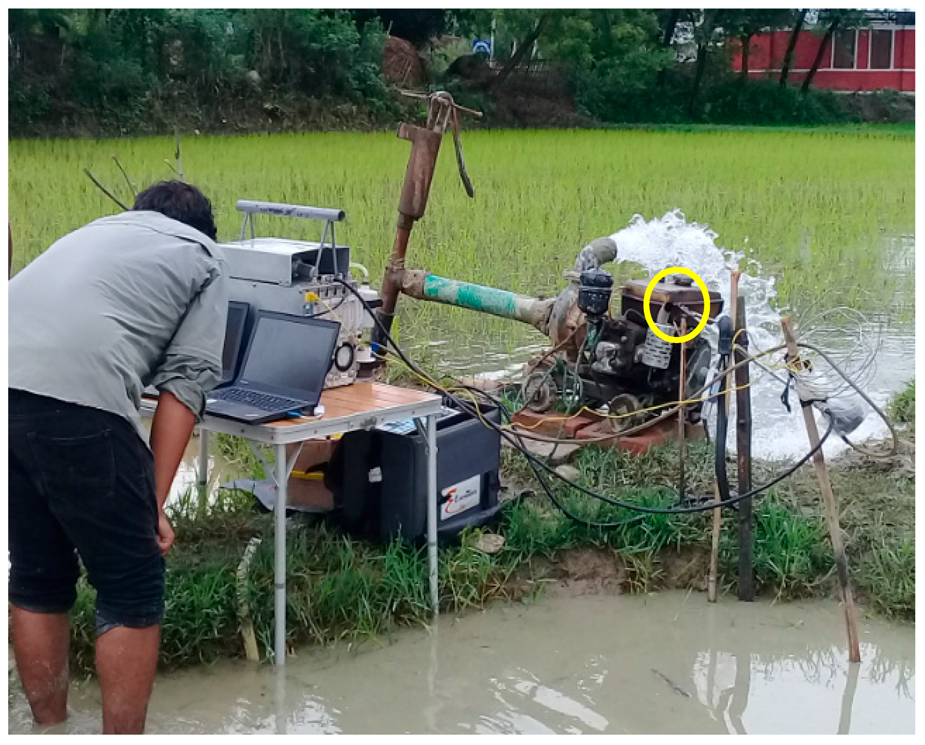
Figure 3.
Real-time measurement of pump emissions in a paddy field, Saptari district, Nepal. Yellow circle indicates Ratnoze1 inlet near to the pump exhaust.
Figure 3.
Real-time measurement of pump emissions in a paddy field, Saptari district, Nepal. Yellow circle indicates Ratnoze1 inlet near to the pump exhaust.

Figure 4.
Box plot showing EFPM2.5 (g/L) (a) and EFBC (g/L) (b) in log scale for all measured pumps. The lower and upper edge of each box represent the 25th and 75th percentiles, respectively; the top and bottom of the whisker represent the 90th and 10th percentiles, respectively. The square box mark within each box represents the average EF and the horizontal mid-line in each box represents the median. EF, emission factors; EFPM2.5, emission factors particulate matter with less than 2.5 µm diameter; EFBC, emission factors black carbon.

Figure 5.
Box plot showing (a) EFCO2 (g/L) and (b) EFCO (g/L) in log scale for all measured pumps. The lower and upper edge of each box represent the 25th and 75th percentiles, respectively; and the top and bottom of the whisker represent the 90th and 10th percentiles, respectively. The square box mark within each box represents the average EF and the horizontal mid-line in each box represents the median. EF, emission factors; EFCO2, emission factors carbon dioxide; EFCO, emission factors carbon monoxide.


Table 1.
Characteristics of diesel irrigation pumps measured during our campaign.
| Pump ID | Depth of Boring (m) | Sampling Date | Pump Manufacturer | Pump Power (kW) | Age of Pump (year) | Fuel Consumption Rate (L/h) | Hours of Operation |
|---|---|---|---|---|---|---|---|
| Pump 1 | 32 | 6-Jul-17 | CD Bharat No1 | 3.73 | 1 | 1.0 | 200 |
| Pump 2 | 32 | 6-Jul-17 | CD Bharat No1 | 3.73 | 1.5 | 1.0 | 150 |
| Pump 3 | 34 | 7-Jul-17 | Kirloskar | 2.98 | 6 | 0.5 | 240 |
| Pump 4 | 34 | 7-Jul-17 | Kirloskar | 3.73 | >10 | 1.5 | 167 |
| Pump 5 | 30 | 8-Jul-17 | CD Bharat No1 | 3.73 | 2 | 1.0 | 150 |
| Pump 6 | 30 | 8-Jul-17 | Birla Power Supply | 2.98 | 5 | 0.5 | 300 |
| Pump 7 | 30 | 9-Jul-17 | Krishiplus China | 3.36 | 6 | 1.0 | 150 |
| Pump 8 | 34 | 10-Jul-17 | Usha Delux | 4.10 | 9 | 1.0 | 100 |
| Pump 9 | 32 | 11-Jul-17 | Super Manokamana Delux | 2.24 | 2 | 0.5 | 300 |
Table 2.
Summary of emission factors for all measured pumps.
| Pump ID | Fuel Used | EFCO2 (g/L) | EFCO (g/L) | EFPM2.5 (g/L) | EFBC (g/L) | MCE (%) |
|---|---|---|---|---|---|---|
| Pump 1 | Diesel | 2592 | 39.1 | 3.72 | 0.46 | 99.6 |
| Pump 2 | Diesel | 2359 | 183.0 | 58.51 | 4.46 | 98.7 |
| Pump 3 | Diesel | 2462 | 121.4 | 5.06 | 0.96 | 98.6 |
| Pump 4 | Diesel | 2145 | 317.4 | 80.33 | 5.86 | 97.2 |
| Pump 5 | Diesel | 2506 | 93.1 | 4.09 | 1.05 | 99.2 |
| Pump 6 | Diesel mixed with gasoline and kerosene | 424 | 1418.9 | 2.67 | 0.24 | 52.0 |
| Pump 7 | Diesel | 2523 | 82.4 | 10.08 | 0.97 | 99.2 |
| Pump 8 | Diesel | 2481 | 106.8 | 6.46 | 3.11 | 99.1 |
| Pump 9 | Diesel | 2471 | 110.0 | 28.06 | 5.76 | 99.2 |
Note: EF, emission factors; EFPM2.5, emission factors particulate matter with less than 2.5 µm diameter; EFBC, emission factors black carbon; EFCO2, emission factors CO2; MCE, modified combustion efficiency.
Table 3.
Comparison of emission factors with previous studies.
| Studies | EFCO2 (g/L) | EF CO2 (g/kg) | EFCO (g/L) | EFPM2.5 (g/L) | EFPM2.5 (g/kWh) | EFBC (g/L) | MCE (%) | CO2 (g/kW) |
|---|---|---|---|---|---|---|---|---|
| Present study | 2218 | 2666 | 274 | 22.1 | 6.58 | 2.5 | 93.6 | 694 |
| Jayarathne et al. 2017 | - | - | - | 5.9 | - | - | - | - |
| Kauret al. 2016 | - | - | - | - | - | - | - | 406 |
| Stockwell et al. 2016 | 2606 | - | - | - | - | 4.7 | 99.20 | - |
| Cai and Wang, 2014 (EF used for NONROAD model for base year 2013) | - | - | - | - | 0.14 | - | - | - |
| Zou et al. 2013 | - | 3300 | - | - | - | - | - | - |
| Ito and Penner, 2005 | - | - | - | - | - | 2.7 | - | - |
| Bond et al. 2004 | - | - | - | - | - | 3.3 | - | - |
EF, emission factors; EFPM2.5, emission factors particulate matter; EFBC, emission factors black carbon; EFCO2, emission factors CO2; MCE, modified combustion efficiency.
© 2019 by the authors. Licensee MDPI, Basel, Switzerland. This article is an open access article distributed under the terms and conditions of the Creative Commons Attribution (CC BY) license (http://creativecommons.org/licenses/by/4.0/).
Share and Cite
MDPI and ACS Style
Adhikari, S.; Mahapatra, P.S.; Sapkota, V.; Puppala, S.P. Characterizing Emissions from Agricultural Diesel Pumps in the Terai Region of Nepal. Atmosphere 2019, 10, 56. https://doi.org/10.3390/atmos10020056
AMA Style
Adhikari S, Mahapatra PS, Sapkota V, Puppala SP. Characterizing Emissions from Agricultural Diesel Pumps in the Terai Region of Nepal. Atmosphere. 2019; 10(2):56. https://doi.org/10.3390/atmos10020056
Chicago/Turabian StyleAdhikari, Sagar, Parth Sarathi Mahapatra, Vikrant Sapkota, and Siva Praveen Puppala. 2019. "Characterizing Emissions from Agricultural Diesel Pumps in the Terai Region of Nepal" Atmosphere 10, no. 2: 56. https://doi.org/10.3390/atmos10020056
Note that from the first issue of 2016, this journal uses article numbers instead of page numbers. See further details here.