Article

Sensitivity of the Reaction Mechanism of the Ozone Depletion Events during the Arctic Spring on the Initial Atmospheric Composition of the Troposphere

1
Key Laboratory for Aerosol-Cloud-Precipitation of China Meteorological Administration, Nanjing University of Information Science and Technology, Nanjing 210044, China
2
Institute of Mechanics, Materials and Civil Engineering, Université catholique de Louvain, Louvain-la-Neuve 1348, Belgium
*
Author to whom correspondence should be addressed.
Atmosphere 2016, 7(10), 124; https://doi.org/10.3390/atmos7100124
Submission received: 1 August 2016 / Revised: 19 September 2016 / Accepted: 25 September 2016 / Published: 30 September 2016

Abstract

:
Ozone depletion events (ODEs) during the Arctic spring have been investigated since the 1980s. It was found that the depletion of ozone is highly associated with the release of halogens, especially bromine containing compounds. These compounds originate from various substrates such as the ice/snow-covered surfaces in Arctic. In the present study, the dependence of the mixing ratios of ozone and principal bromine species during ODEs on the initial composition of the Arctic atmospheric boundary layer was investigated by using a concentration sensitivity analysis. This analysis was performed by implementing a reaction mechanism representing the ozone depletion and halogen release in the box model KINAL (KInetic aNALysis of reaction mechanics). The ratios between the relative change of the mixing ratios of particular species such as ozone and the variation in the initial concentration of each atmospheric component were calculated, which indicate the relative importance of each initial species in the chemical kinetic system. The results of the computations show that the impact of various chemical species is different for ozone and bromine containing compounds during the depletion of ozone. It was found that CH3CHO critically controls the time scale of the complete removal of ozone. However, the rate of the ozone loss and the maximum values of bromine species are only slightly influenced by the initial value of CH3CHO. In addition, according to the concentration sensitivity analysis, the reduction of initial Br2 was found to cause a significant retardant of the ODE while the initial mixing ratio of HBr exerts minor influence on both ozone and bromine species. In addition, it is also interesting to note that the increase of C2H2 would significantly raise the amount of HOBr and Br in the atmosphere while the ozone depletion is hardly changed.

1. Introduction

Due to its unique role in the lower atmosphere, ozone has become the focus of the scientific community since its first discovery by Schoenbein in 1840 [1]. In the stratosphere, ozone is called “good ozone”, as it is capable of absorbing most of the Ultra-Violet (UV) radiations from the sun and, thus, protecting life on earth. Moreover, ozone plays a role in converting radiation to heat so that the top of the upper part of the stratosphere is warmed. As a result, a temperature inversion is formed in the stratospheric layer, which leads to its existence. On the contrary, the troposphere ozone contains a kind of pollutant that has a mixing ratio of 20–60 ppb on average (ppb = parts per billion) [2]. It was found by Lippmann [3] that an exposure of healthy adults to a 100 ppb ozone environment for several hours would lead to a severe reduction of the lung function. Furthermore, this harmful effect brought about by an excessive amount of the tropospheric ozone accumulates when the exposure time is extended. Apart from this, ozone in the troposphere also destroys living tissue, causing eye irritation and chest pain to individuals [4]. Therefore, tropospheric ozone is also called “bad ozone”. Since ozone in the troposphere originates from several precursors such as hydrocarbons and nitrogen oxides (NOx) that are produced from human activities such as gasoline vapors, power plants using fossil fuel and automobile emissions, due to the growing population and industrial activities, the background level of the tropospheric ozone has more than doubled since 1900 [5].
In the 1980s, an abnormal decline in the mixing ratio of the tropospheric ozone in polar regions was reported from various sites such as Barrow, Alaska [6] and Alert, Canada [7] during springtime. In these observations, the surface ozone mixing ratio was found to drop within a couple of days from its background level (∼40 ppb) to less than 1 ppb or even below the detection limit, which is then termed “ozone depletion events” (ODEs). Furthermore, a strong enhancement of halogen species, in particular of bromine containing compounds, in the troposphere during ODEs was also noticed [8]. A strong correlation between the decline of ozone and the rise of the bromine amount in the troposphere was found, which indicates the importance of bromine for the destruction of ozone. Later on, Hönninger and Platt [9] revealed that bromine monoxide (BrO) is involved in an auto-catalytic reaction cycle in which ozone is consumed without any loss of bromine. It was suggested by Hönninger and Platt [9] that BrO participates in the self-reactions,
BrO + BrO Br 2 ( or   2 Br ) + O 2
in which Br2 or Br atoms are formed. In the presence of sunlight, Br2 is rapidly photolyzed and converted to Br which continues to destroy ozone in the troposphere as follows,
Br 2 + h ν 2 Br
Br + O 3 BrO + O 2
However, the Reactions (R1)–(R3) cannot explain the sharp increase of bromine during ODEs. Thus, apart from these reactions, it is supposed that the gas-phase hypobromous acid (HOBr) formed by the oxidation of BrO is also able to activate bromide from various polar substrates such as the suspended aerosols and ice/snow-covered surfaces, leading to an explosive increase of the total bromine amount and also a rapid ozone depletion in the troposphere. This process can be expressed as
Br + O 3 BrO + O 2 BrO + HO 2 HOBr + O 2 HOBr + H + + Br mp Br 2 + H 2 O Br 2 + h ν 2 Br Net : O 3 + HO 2 + H + + Br + h ν mp 2 O 2 + Br + H 2 O
In the above reaction sequence, “mp” represents multiphase reactions which occur in or on the suspended aerosols and the surfaces covered by ice and snow. It is evident that a bromide ion stored in the substrates is activated by HOBr through Reaction (R4). Consequently, it is converted to Br which resides in the troposphere and consumes ozone. As a result, the total gas-phase bromine loading in the troposphere rises exponentially. This reaction sequence is called “bromine explosion” mechanism [9,10,11,12].
The tropospheric ODEs and the associated bromine explosion phenomenon have a great influence on life on earth and also the climate of polar regions. During ODEs, the oxidation ability of the atmosphere in the troposphere is dominated by the bromine containing compounds instead of ozone. As a result, more reactive gas mercury (RGM) is formed and then deposited on the ground surface. In late spring or summertime, due to the increase in temperature, the deposited RGM is then carried by the melted snow, flowing into the ocean. Through the oceanic circulation, RGM would consequently enter the bodies of people at mid-latitudes, damaging their health. Furthermore, as ozone is also a type of greenhouse gas which warms the surface of polar regions, the decline of the ozone mixing ratio during springtime would modify the melting speed of glaciers so that the climate of polar regions is influenced.
In order to investigate the physical and chemical processes related to ODEs, a large amount of studies have been performed previously. Generally, the occurrence and termination of ODEs are determined by the joint effect of the local chemistry, vertical turbulent mixing, and long-range transport. As discussed above, the major chemical pathways for the production and destruction of ozone during ODEs are the brominated Reactions (R1)–(R4) [10,11,12]. This bromine chemistry consists of gas-phase reactions as well as heterogeneous reactions for releasing bromine to the ambient air. The importance of vertical mixing in the boundary layer was first discovered by Lehrer et al. [13] by using the one-dimensional model FACSIMILE. Their computational results indicated for the region above the boundary layer that the formation of a temperature inversion causes a decrease of the turbulent diffusivity. Therefore, the ozone-rich air in the free troposphere is hardly transported into the boundary layer, which favors the occurrence of ODEs therein. Apart from these two mechanisms, ODEs are also influenced by the long-range transport of the air. Strong et al. [14] and Morin et al. [15] pointed out that the ODEs observed around Alert, Canada originate from the air which had previous contact with the newly-formed fresh sea ice northwest of Alert. In contrast to that, when the ozone-rich air influenced by the inland multi-year sea ice is transported from the south to Alert, the low-ozone episodes terminated. Their conclusions are also confirmed through the observations made by Jones et al. [16]. A thorough review of the existing studies on ODEs is given by Platt and Hönninger [10], Simpson et al. [11] and Abbatt et al. [12].
Recently, studies on the sensitivity of the mixing ratios of ozone and principal bromine containing compounds during ODEs on the initial amount of bromine in the atmospheric composition were performed [17]. In addition, the dependence of the ozone depletion rate on the prescribed fluxes of halogen species such as Br2 and BrCl from the underlying surfaces was investigated by Evans et al. [18], and Piot and Von Glasow [19,20]. In these studies [17,18,19,20], it is found that the occurrence of ODEs is deeply influenced by the change of the initial atmospheric composition of the troposphere. However, this kind of sensitivity study is normally performed in a “brute force” way in which the initial mixing ratio of each component of the atmosphere is varied by a certain extent to see the corresponding changes in the computational results of the model. This approach is convenient but also extremely time-consuming. In addition, the change of the system due to the variation of the different species concentrations is incomparable as the magnitude of the variation belonging to each constituent differs a lot. Therefore, in the present study, we adopted a more systematic and economical approach, namely the concentration sensitivity analysis in a box model, to reveal the dependence of ozone and bromine species on the initial mixing ratio of each species in the troposphere. In the concentration sensitivity analysis, the percentage change of the mixing ratio of specified species such as ozone caused by a 1% change in the initial species concentration is computed. Thereby, the importance of each constituent in the initial composition of the atmosphere for the depletion of ozone in the Arctic spring is identified. Moreover, the sensitivity coefficient obtained in this analysis is a dimensionless variable so that a comparison of the relative importance of each constituent in the initial air composition for ozone and bromine species can be performed.
The manuscript is organized as follows. In Section 2, the mathematical equations used in the present study are given. The configuration of the model is also presented in this section. The most significant computational results are shown in Section 3. The importance of each initial species concentration for the mixing ratios of ozone and bromine species during ODEs is indicated by the values of the sensitivity coefficients. At the end of this section, we modify the initial mixing ratios of the most influential/special species which are discovered by the concentration sensitivity analysis to make a comparison between the simulation results before and after the modification. At last (Section 4), the major conclusions drawn from the present study are given. Future improvements of the present model are also discussed.

2. Mathematical Models and Methods

The chemical reaction system used in the present study can be expressed as
d c d t = f ( c , k ) + E
with the initial condition c t = 0 = c 0 . In Equation (1), c is a column vector consisting of species concentrations, and its i-th element, c i , denotes the concentration of the i-th species. k in Equation (1) represents a vector of reaction rate constants, and its j-th element, k j , corresponds to the rate coefficient of the j-th reaction. t in Equation (1) denotes time, and E is the source term for the local emissions from the underlying surface. After implementing a reaction mechanism of ODEs in the box model KINAL (KInetic aNALysis of reaction mechanics) [21] and solving Equation (1), we are able to capture the temporal evolutions of ozone and principal bromine species in the ODE event. The adopted reaction mechanism in the present study is taken from previous studies [13,17,22] and consists of 92 reactions among 39 chemical species. The full reaction mechanism is listed in Table A1 in the Appendix. This mechanism includes both the gaseous reactions and the heterogeneous reactions occurring on the surfaces of polar substrates. The rate coefficients of the gas-phase reactions are estimated by using the Arrhenius equation [23] based on the latest kinetic data for atmospheric chemistry [24]. A constant temperature of 258 K is assumed for the calculation of the gas-phase reaction rates in the mechanism [13].
In contrast to the gas-phase reactions, the estimation of the rates of the heterogeneous reactions depends on the properties of the suspended aerosols and the local meteorological parameters such as the wind speed and the stability of the boundary layer. For the heterogeneous reactions occurring on the aerosol surfaces (reactions No. 14 and No. 90 in Table A1 in the Appendix), the aerosol volume density under typical Arctic springtime conditions, V aerosol = 10 5 cm3·m−3 was assumed according to Staebler et al. [25], and the average aerosol radius r is set to 0.3 μm in the present model. The rate constant of the heterogeneous reactions occurring on the aerosols is calculated as
k aerosol = ( r D g + 4 v therm γ ) 1 α eff , aerosol
where D g = 0.2 cm2·s−1 denotes the gas-phase molecular diffusivity, and v therm is the mean molecular speed. γ represents the uptake coefficient of HOBr or BrONO2 on aerosols. For the HOBr + HBr reaction (reaction No. 14 in Table A1), the estimation of the HOBr uptake coefficient is based on the method of Hanson et al. [26] in which the value of γ depends on the rate of the aqueous reaction between HOBr and HBr. For the hydrolysis reaction of BrONO2 on the aerosol surface (reaction No. 90 in Table A1), a constant uptake coefficient 0.06 is taken from Sander and Crutzen [27]. α eff , aerosol in Equation (2) is the surface area density of the suspended aerosols, and it is estimated as
α eff , aerosol = V aerosol × 3 / r = 10 4 m 1
With respect to the heterogeneous reactions occurring on the ice/snow-covered surfaces (reactions No. 15 and No. 92 in Table A1 in the Appendix), it is necessary to consider the aerodynamic resistance r a , quasi-laminar resistance r b due to the molecular diffusion, and the surface resistance r c . Parametrization from previous model studies [13,17,22] for these heterogeneous reactions is adopted in the present study. In this parametrization, the wind speed 8 m·s−1 is assumed [28], and a constant value of 10−5 m is used for the roughness of the ice surface [29,30,31]. A constant uptake coefficient 0.06 is taken after Sander and Crutzen [27] for HOBr as well as BrONO2 on the ground ice surface. It is also assumed in the model that the bromide storage in the acidic ice/snow-covered surfaces is inexhaustible [13,17,22]. Apart from this, the parametrization adopted in the model still requires the prescription of the height of the boundary layer and the surface layer. In the present box model study, a typical polar boundary layer height of 200 m is used for defining the top of the computational domain. Furthermore, the height of the surface layer is assumed to be 10% of the boundary layer height, i.e., 20 m [29].
In our model, photolysis frequencies were estimated by assuming a fixed solar zenith angle (SZA), 80°, which was also used in the earlier study of Lehrer et al. [13]. The evaluation of the photolysis frequencies J is performed by using a three-coefficient formula from Röth’s ART (Anisotropic Radiation Transfer) model [32,33] with albedo =1.0:
J = J 0 exp ( b [ 1 sec ( c χ ) ] )
In Equation (4), χ is the SZA. The coefficients J 0 , b, c are determined from the ART model at χ = 0°, 60° and 90°. The values of the coefficients, J 0 , b and c, for the estimation of the photolysis reactions are listed in Table A2 in the Appendix.
The initial composition of the atmosphere used in the model, listed in Table 1, represents a typical Arctic condition. A small amount of bromine (0.3 ppt Br2 and 0.01 ppt HBr) is prescribed in the model which plays the role of triggering the bromine explosion mechanism. Nitrogen oxides (NOx), HONO, H2O2 and HCHO were found to be emitted from the underlying surfaces of polar regions [34,35,36,37]. Thus, fluxes of these species emitted from the ice/snow-covered surfaces of the Arctic are also included in the model (see Table 2). The emission rates of these species are estimated according to previous measurements [34,35,36,37], and the emission of HONO is assumed to be equal to that of NO2 [36].
After the initialization of the model, Equation (1) is solved in the box model KINAL using a fourth-order semi-implicit Runge–Kutta scheme [38]. Then, the temporal behavior of ozone and bromine containing compounds are obtained. Afterward, we performed a concentration sensitivity analysis on the present reaction mechanism to identify the most influential/special atmospheric components in the initial atmosthe phere for ozone and bromine species during ODEs. The definition of the relative concentration sensitivity is as follows,
S ˜ i j ( t ) = ln c i ( t ) ln c j 0 = c j 0 c i ( t ) c i ( t ) c j 0
In the above equation, c i ( t ) is the concentration of the i-th chemical species at the time t, and c j 0 denotes the initial concentration of the j-th species. Furthermore, S ˜ i j is the relative concentration sensitivity, which is a dimensionless parameter representing the percentage change of the i-th species concentration due to 1% variation of the initial concentration of the j-th species. By introducing S ˜ i j , we were able to reveal the importance of the initial concentration belonging to each component of the atmosphere for the mixing ratios of ozone and bromine species during ODEs. In KINAL, the relative concentration sensitivity is computed using a Decomposed Direct Method [39], which has been proved robust and highly efficient [40].
After obtaining the relative concentration sensitivity on each initial constituent of the atmosphere, we chose the species with the largest sensitivities and the species with the most special characteristics as candidates for further investigations. The initial mixing ratios of these important species are multiplied by a factor of 1.5 or divided by 2 to observe the corresponding changes of the kinetic system. In the present study, we focus on the deviations of the mixing ratios of ozone and three principal bromine species (BrO, HOBr andBr) during the ODE event.
In the next section, the computational results are presented and discussed.

3. Results and Discussion

In this section, we first show the temporal evolution of the principal chemical species such as ozone in the 200 m boundary layer during the ODE. Then, the relative concentration sensitivities of ozone, BrO and HOBr on the initial mixing ratios of the atmospheric components are displayed. Finally, the initial concentrations of the most influential/special species are varied so that the response of the system is captured and discussed.

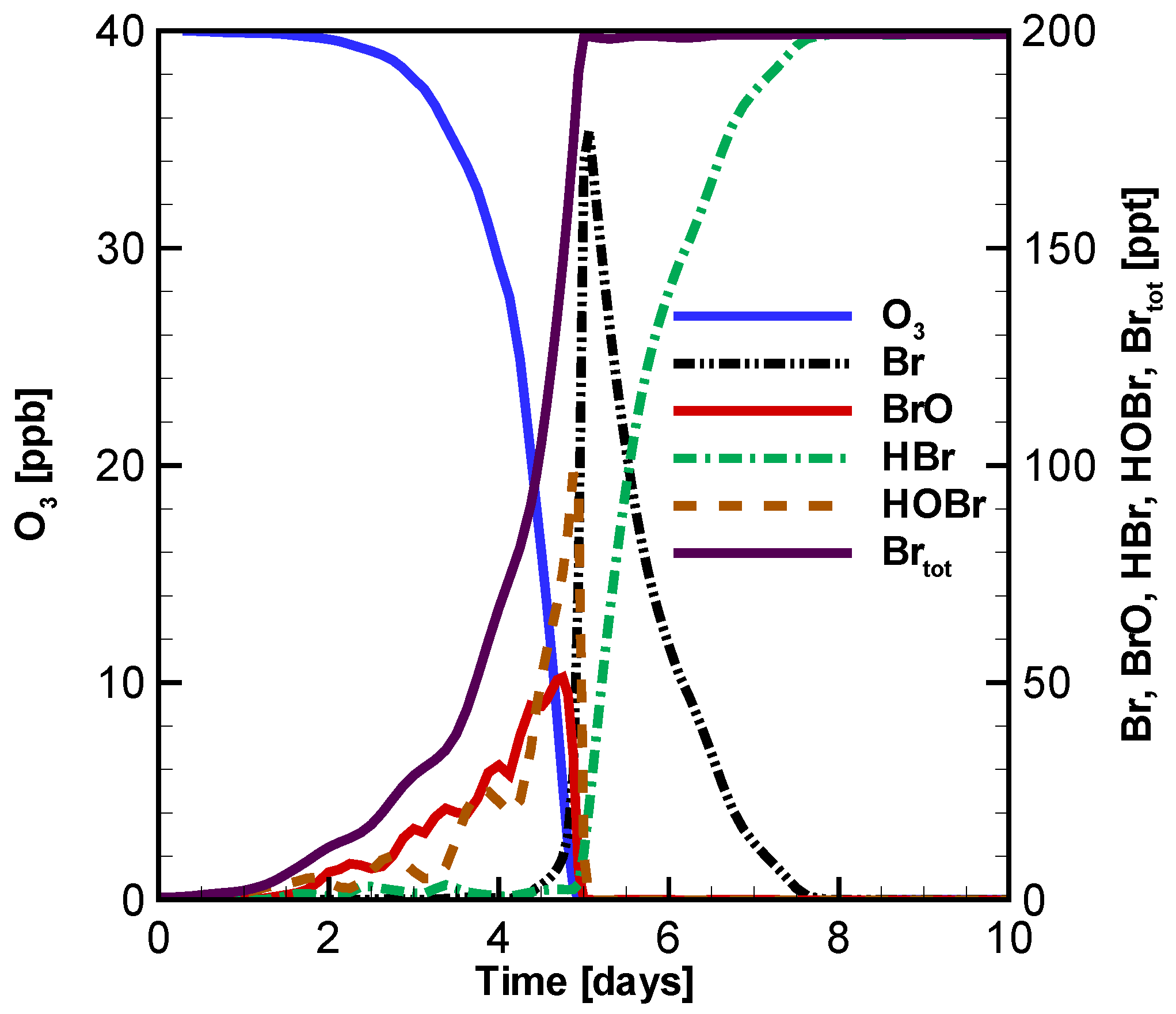
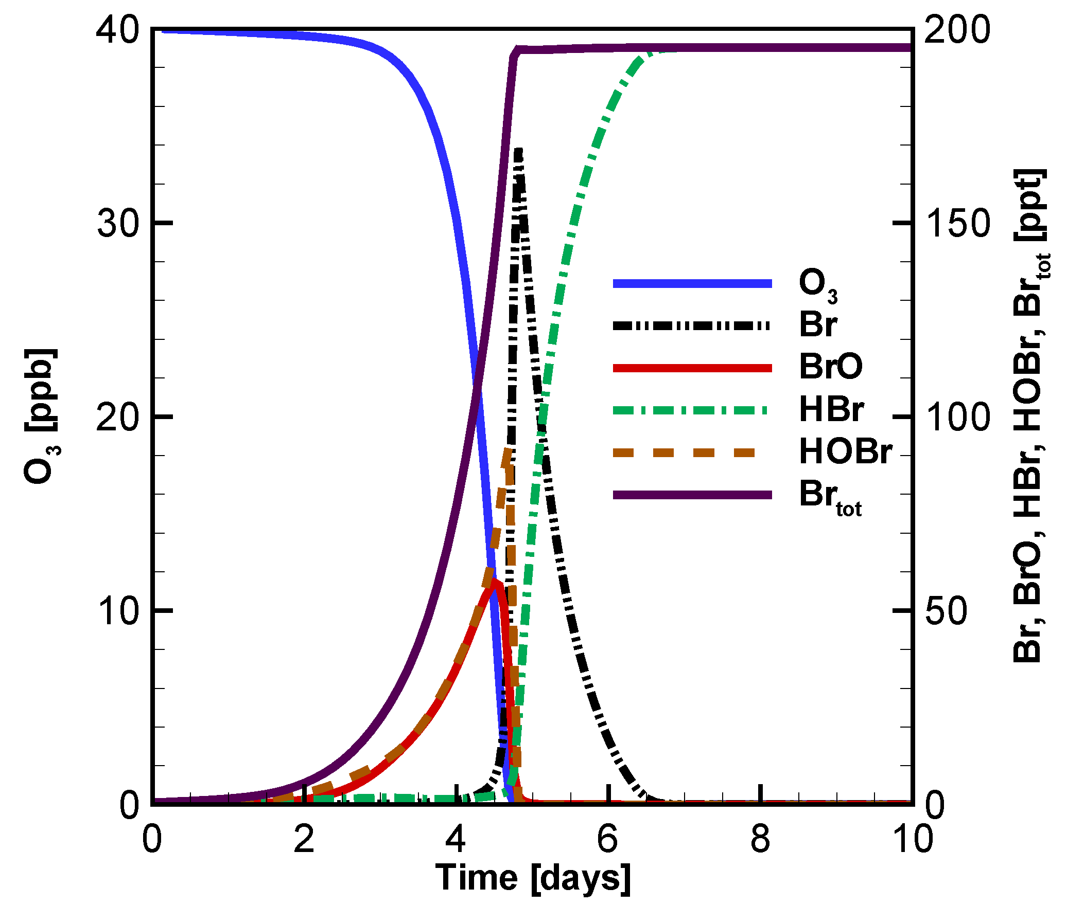
3.1. Temporal Evolution of Ozone and Principal Bromine Species

Figure 1 shows the development of the mixing ratios of ozone and principal bromine species with time. Since this result has been presented and discussed in our previous publications [17,22], we give in the present manuscript only a brief outline of their most important features. It is seen in Figure 1 that ozone starts to drop significantly after day 3 before which the ozone depletion rate is less than 0.1 ppb·h−1. In the early stage of the simulation (before day 3), as ozone is abundant in the boundary layer, the formation of BrO is able to proceed. Therefore, BrO and HOBr increase steadily, which makes them the major contributions to the total bromine amount in the troposphere. In contrast to that, Br atoms can hardly be observed in the early stage since they react rapidly with the present ozone. After day 3, HOBr reaches its peak value of 92 ppt. Consequently, the activation of bromide from the ice/snow-covered surface is strongly enhanced. As a result, the total bromine amount in the ambient air increases explosively, thus speeding up the depletion of ozone. The rate of ozone depletion in this time period exceeds 0.1 ppb·h−1, and reaches the maximum of 1.9 ppb·h−1. After 4.6 days, ozone drops to a level lower than 10% of its background value (4 ppb). The formation of BrO tends to be prohibited. Thus, the mixing ratios of BrO and HOBr decline instantly to a value lower than 1 ppt. Due to the photolytic decomposition of BrO, Br builds up to be the major bromine species and amounts to 170 ppt after 4.8 days. Later on, this amount of Br atoms is converted to HBr through the scavenging process by aldehydes in the troposphere. Thus, HBr becomes the major bromine species remaining in the boundary layer after the ODE, which is in accordance with the previous measurement [41].
In order to investigate the influence brought about by the variation of SZA, we also conducted a simulation by using a varying SZA value. In this simulation, an initial χ 0 value, 85.5° is assumed for the date of April 1 at 80° N. According to Röth’s model [32,33], SZA at this location varies as
χ = χ 0 4.11 × 10 6 time + 6.5 cos ( 2 π / 86400 × time )
The first term on the right-hand side (RHS) of Equation (6) is the initial SZA value. The second term in the RHS denotes the SZA change for different days in April. The third term is the daily change of SZA. The result with varying SZA in the 200 m boundary layer is presented in Figure A1 in the Appendix. It is seen in Figure A1 that although the ozone depletion is prolonged a little bit by approximately half a day after the inclusion of the SZA variation, there has been little change in the temporal behavior of ozone and halogen species concentrations after the modification. Thus, the simulation results with fixed value of SZA are capable of describing the main features of ODEs, and the time used in the present model can be considered as equal to the real time. Thus, we continue using the reaction mechanism with the fixed SZA value in the following exploratory simulations.
In the next section, a concentration sensitivity analysis is applied on the present reaction mechanism for the time period during the depletion of ozone.

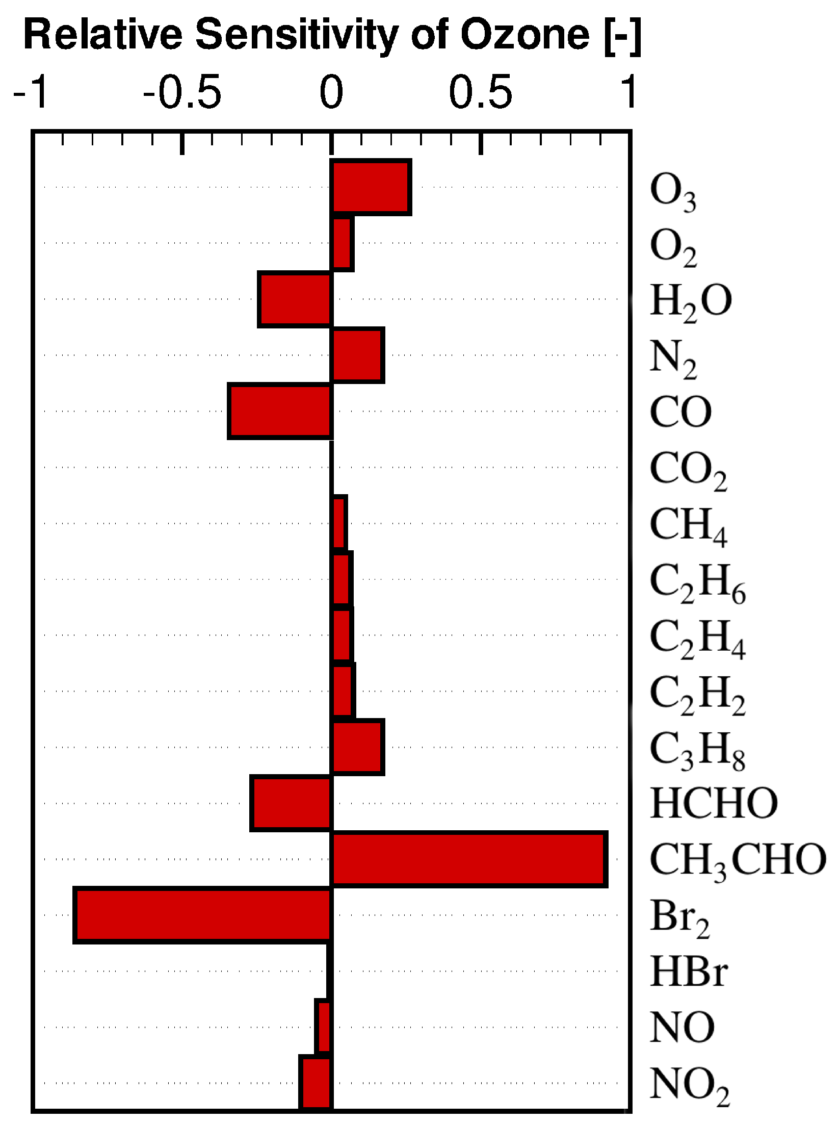
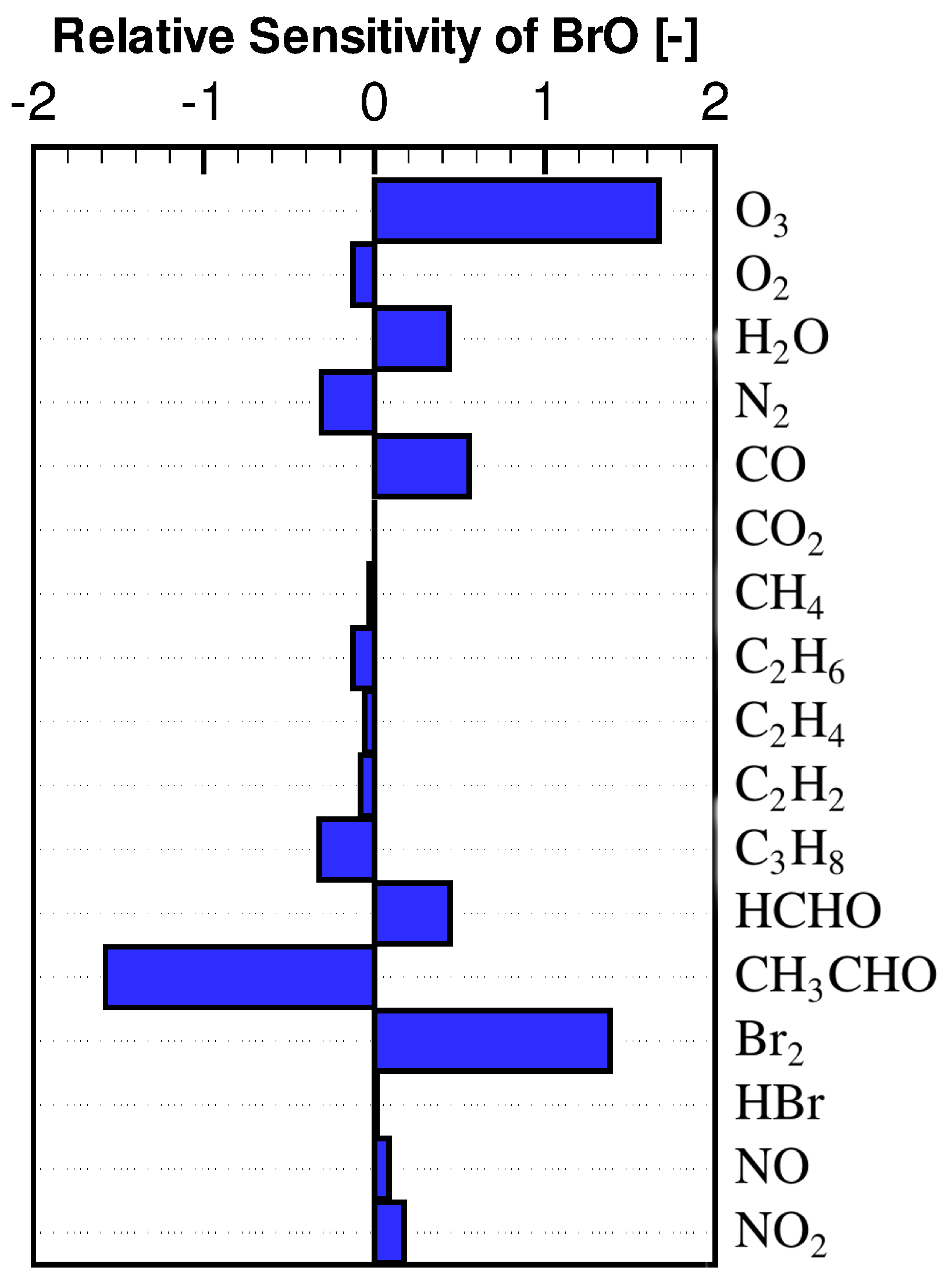
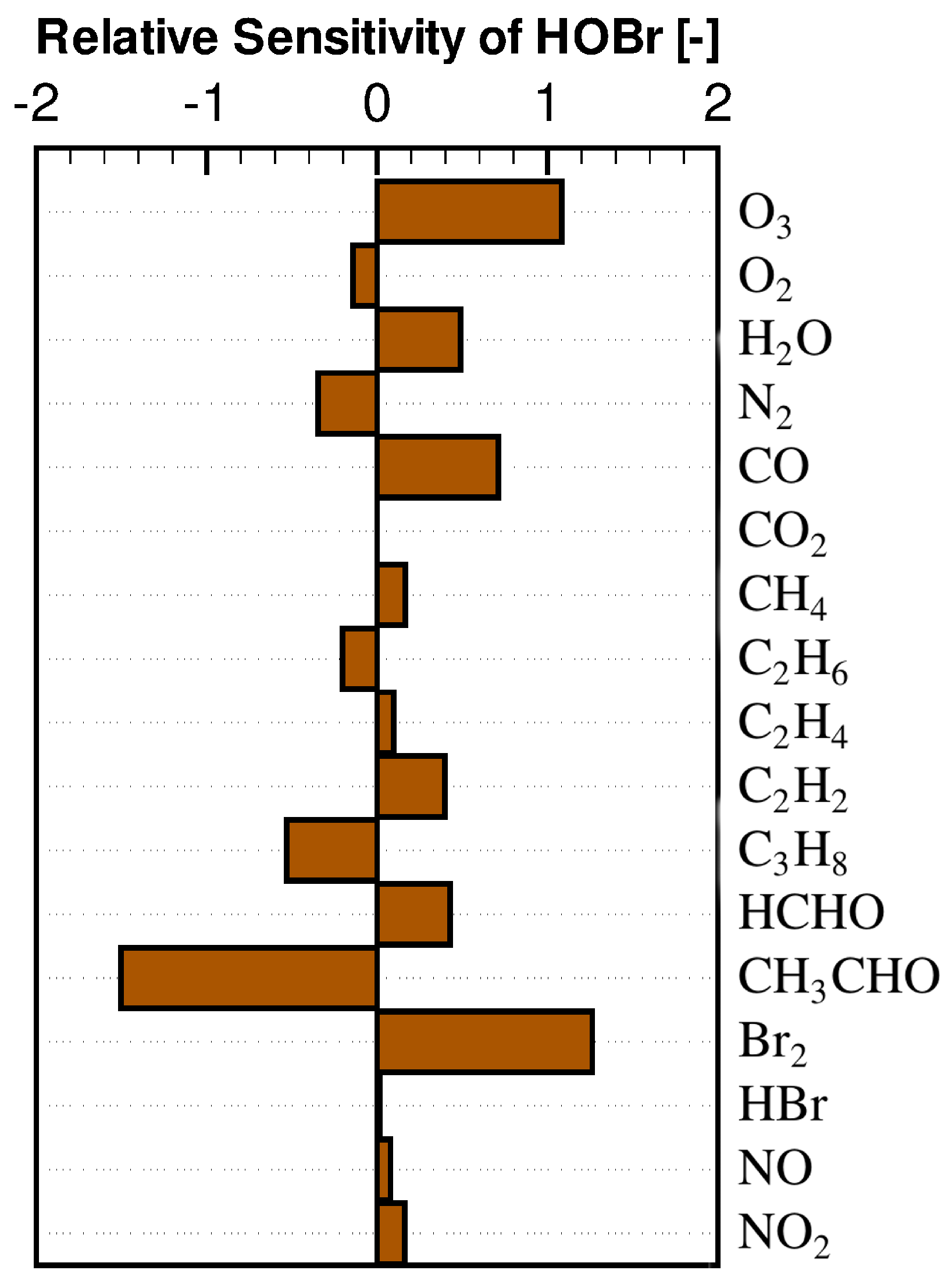
3.2. Concentration Sensitivity Analysis of the Mixing Ratios of Ozone and Bromine Containing Compounds during the ODE

Figure 2 displays the relative concentration sensitivities of ozone in the ambient air on day 4 which resides in the depletion period of ozone on each component of the initial atmospheric composition. It is seen that for the ozone mixing ratio during the ODE, the initial concentration of CH3CHO has the largest absolute value of the relative concentration sensitivity. This means that the ozone during the ODE is mostly influenced by the initial concentration of CH3CHO. In addition, the sign of the sensitivity coefficient corresponding to CH3CHO is positive, which indicates that an increase of the initial concentration of CH3CHO enhances the ozone mixing ratio during ODEs. The reason is attributable to the absorption of Br by CH3CHO:
Br + CH 3 CHO O 2 HBr + CH 3 CO 3
Br is a chemical species that directly consumes ozone. Therefore, an increase of the initial concentration of CH3CHO leads to a decrease of the quantity of Br available for the consumption of ozone during ODEs. As a result, the depletion of ozone is retarded, and the mixing ratio of ozone would increase. This finding is in good agreement with the conclusions obtained by Shepson et al. [42] saying that CH3CHO plays a major role as the sink of the reactive bromine in the Arctic Ocean boundary layer. In contrast to that, it is interesting to note that the sensitivity coefficient of ozone for HCHO has a negative value on day 4 (see Figure 2). This shows that, different from CH3CHO, an increase of the initial concentration of HCHO would decrease the mixing ratio of ozone, and, thus, speed up the ODE. By comparing the reactions of the used mechanism related to CH3CHO and HCHO, we found that, for CH3CHO, the Reaction (R5) outlined above is the major chemical pathway which influences the ozone mixing ratio. As discussed above, through Reaction (R5), the active bromine atoms are scavenged by CH3CHO and converted to HBr, leading to the slow down of the ODE. However, for HCHO the reaction between HCHO and Br is as follows:
Br + HCHO O 2 HBr + CO + HO 2
Although Br is also converted to the inert bromine species HBr through Reaction (R6), CO and HO2 are produced. As CO is able to react with hydroxyl radicals (OH) in the troposphere forming HO2, the total amount of HO2 in the troposphere is strongly enhanced during ODEs when Reaction (R6) proceeds. Since HO2 is capable of oxidizing BrO to HOBr, the increase of the initial mixing ratio of HCHO would strengthen the formation of HOBr, and, thus, speed up the bromine explosion mechanism. As a result, the depletion of ozone is accelerated.
According to the sensitivity values depicted in Figure 2, the second important initial component of the troposphere for the ozone mixing ratio during ODEs is Br2. This is not entirely surprising as the initial Br2 plays the role of stimulating the bromine explosion mechanism which consequently leads to the consumption of ozone. Thus, the increase of the initial Br2 in the atmosphere would significantly speed up the occurrence of ODEs. In contrast to Br2, the sensitivity of the ozone mixing ratio on HBr is negligible. This is because HBr is inert in the reaction cycle of the ozone depletion as it can be hardly reactivated and photodecomposed. The chemical species CO also has a relatively high sensitivity among the initial components of the atmosphere. This is attributed to the speeding up of the bromine explosion mechanism via the reactions
CO + OH O 2 CO 2 + HO 2
and
HO 2 + BrO HOBr + O 2
which has been discussed above. Apart from these species, the initial mixing ratio of water vapor (H2O) has a negative sensitivity as it is the major sink of the Ox family (O3 + O(1D)) in the troposphere [2]. It is also interesting to note that the mixing ratio of ozone during ODEs depends negatively on the initial concentrations of nitrogen oxides (NO + NO2), which means that the role of the nitrogen oxides during ODEs is to accelerate the ODE and decrease the ozone mixing ratio instead of forming ozone. This ozone-consumption effect brought about by nitrogen oxides during ODEs is caused by the hydrolysis of BrONO2, namely
BrONO 2 + H 2 O mp HOBr + HNO 3
during which HOBr is formed. As a result, the bromine explosion and the following ozone consumption are enhanced in the presence of nitrogen oxides. This finding is also consistent to our previous box model study [17] in which the addition of the nitrogen chemistry is found to advance the ODE. In a recent study of Custard et al. [43], by performing two simulation scenarios with different input profiles of NOX, they stated that the rate of ozone loss is decelerated when the mixing ratio of NOX increases. However, in both of the two simulations performed by Custard et al. [43], the input NOX profiles possess the values more than 50 ppt, reaching the maximum as high as 1600 ppt. Thus, the BrO + NO2 reaction which generates BrONO2 in their simulations is insensitive to the quantity of NOX, as the amount of NOX is abundant. As a result, it is not surprising to find in their model that the increase of NOX tends to decelerate the ODE as the additional NOX mostly plays the role of forming ozone. In our present study, the initial amount of NOX is 15 ppt so that the formation of BrONO2 via the BrO + NO2 reaction depends heavily on the availability of NOX. Thus, the increase of NOX in our present model tends to enhance the hydrolysis of BrONO2, leading to a speeding up of the ODE and the enhancement of the bromine explosion mechanism.
The relative concentration sensitivities of BrO on each component of the initial atmospheric composition are displayed in Figure 3. Compared to the results shown in Figure 2, the sensitivity coefficients of all components except ozone have an opposite sign. This is due to the fact that the formation of BrO is correlated with the decline of ozone. In addition, it is shown in Figure 3 that the sensitivity coefficient of BrO on the initial mixing ratio of ozone is relatively large and possesses a positive sign. This is expected as the major formation pathway of BrO is the reaction Br + O3 → BrO + O2, which requires the presence of ozone. These findings are in agreement with the conclusions obtained by Hausmann and Platt [44], suggesting that BrO is an important indicator of ODEs as the enhancement of BrO requires the presence of ozone and a drop of the ozone mixing ratio.
At the end of this section, attention is paid to the relative concentration sensitivities of HOBr on the initial atmospheric composition (see Figure 4). It is found that the results obtained for HOBr are similar to those for BrO shown in Figure 3. However, the initial concentrations of CH4, C2H4 and C2H2 have positive sensitivities for the HOBr mixing ratio while negative values are obtained for the mixing ratio of BrO. By investigating the reaction mechanism used in the present study, we found that CH4 participates in the reaction sequence as follows:
CH 4 + OH O 2 CH 3 O 2 + H 2 O
CH 3 O 2 + BrO HOBr + HCHO + 0.5 O 2
Therefore, through Reactions (R10) and (R11), BrO is converted to HOBr, which explains the different signs of the sensitivity coefficients for the mixing ratios of BrO and HOBr. With respect to C2H4 and C2H2, these two species are involved in the reactions
Br + C 2 H 4 2.5 O 2 2 CO + HO 2 + HBr + H 2 O
and
Br + C 2 H 2 2 O 2 2 CO + HO 2 + HBr
In these two reactions, not only the major reactant of BrO, namely Br atoms, are consumed, but also HO2 is formed. As HO2 is able to oxidize BrO to HOBr, these two reactions with the involvement of C2H4 and C2H2 cause a speciation shift from BrO to HOBr, leading to negative sensitivities of these two species for BrO and positive sensitivities for HOBr.
Next, we chose the most influential species with the largest absolute values of the sensitivity coefficients, CH3CHO and Br2, and the most special species, C2H2, which is identified in the concentration sensitivity analysis to perform numerical tests by multiplying their initial mixing ratios by 1.5 and 0.5 to study the corresponding changes in the concentrations of ozone and principal bromine species.

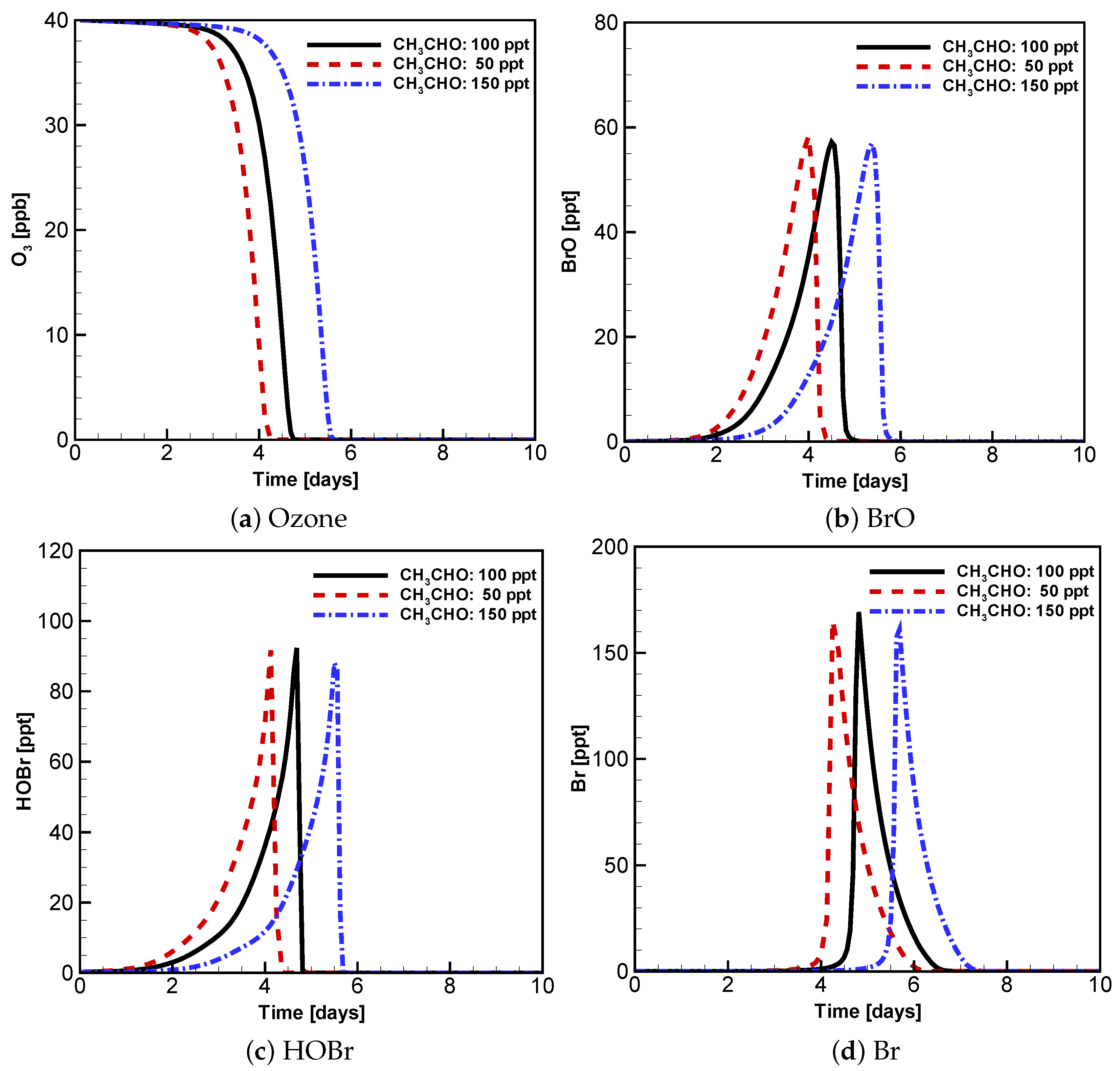
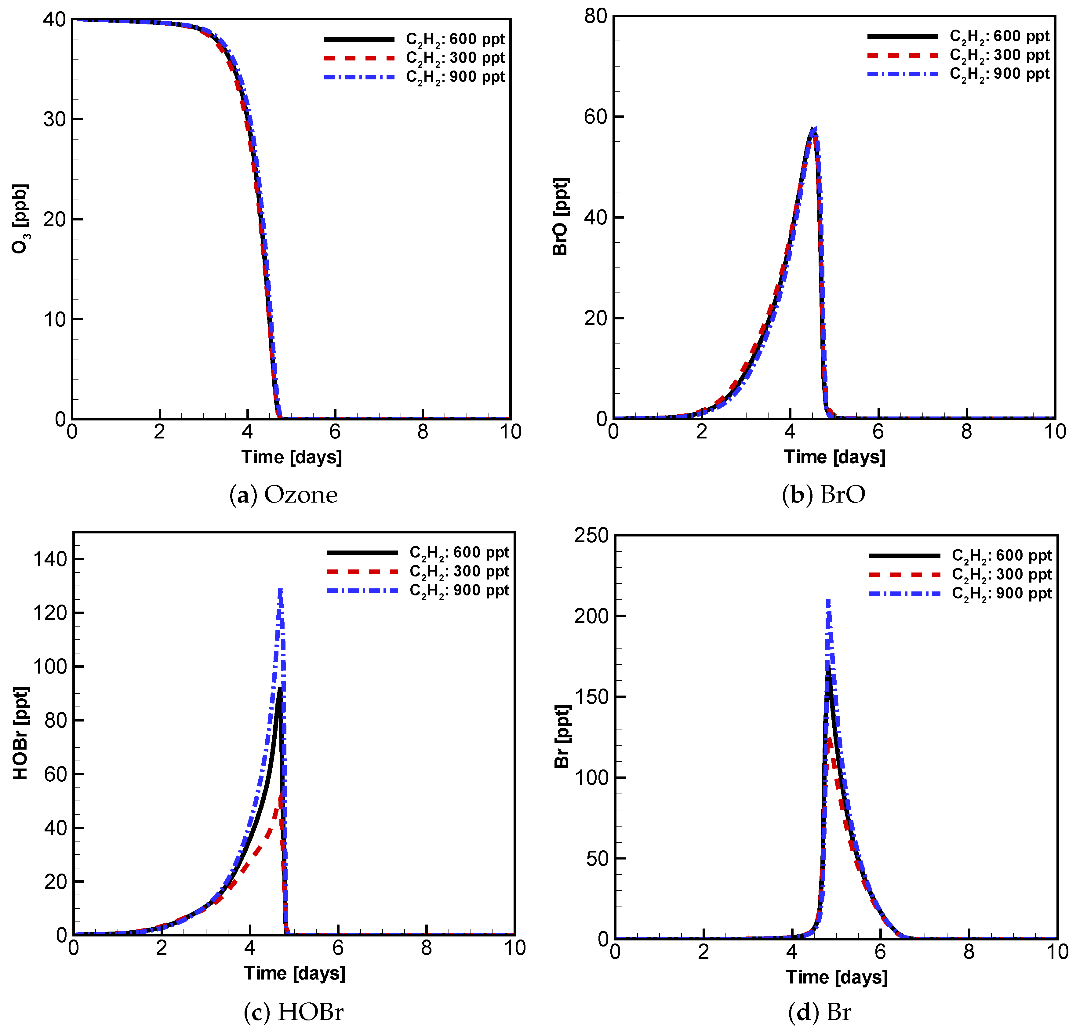
3.3. Evolution of Ozone, BrO, HOBr and Br with Different Initial Atmospheric Composition

Figure 5 shows the temporal behavior of ozone and principal bromine species (BrO, HOBr and Br) before and after the modification of the initial mixing ratio of CH3CHO. It is evident in Figure 5a that the change in the initial CH3CHO causes a significant acceleration or retardation of the ODE. The ozone in the 200 m boundary layer declines to a level lower than 4 ppb after four and 5.5 days when the initial mixing ratio of CH3CHO changes to 50 ppt and 150 ppt, respectively. However, from Figure 5a, it is also found that the acceleration or deceleration of the ODE is mostly attributable to the shortening of the induction stage, which resides before the significant decline of ozone. The simulated ozone depletion rates under different initial conditions are actually similar. Meanwhile, in Figure 5b–d, we found that, although the increase of the bromine species such as BrO and HOBr are advanced or delayed after the modification of the initial CH3CHO, the peak values of these principal bromine species during ODEs are approximately equal to that without the modification. Therefore, we conclude that the change in the initial mixing ratio of CH3CHO leads to a significant variation in the onset of the ODE while the depletion rate of ozone and the peak values of the principal bromine species during ODEs are only slightly influenced.
Simulation results after changing the initial mixing ratio of Br2 from 0.3 ppt to 0.15 ppt and 0.45 ppt are also obtained (not shown here). We found that the effects on the mixing ratios of ozone and bromine species caused by the modification of the initial Br2 are similar to those with the modification of the initial CH3CHO shown in Figure 5. It is observed that when the initial Br2 is reduced from the original value 0.3 ppt to 0.15 ppt, the depletion of ozone occurs one day later than with the original Br2 value, starting approximately during day 4. In contrast, a prescribed 0.45 ppt Br2 in the initial composition of the troposphere leads to an advancement of the ODE, which occurs after 2.6 days. However, similar to the simulation scenario with the CH3CHO variations, little changes about the peak values of principal bromine species and the depletion rate of ozone after the variation in the initial mixing ratio of Br2.
Finally, we chose a special chemical species indicated by the concentration sensitivity analysis, C2H2, to perform the numerical tests. It is seen in Figure 2 and Figure 3 that the relative concentration sensitivities of ozone and BrO on the initial mixing ratio of C2H2 are lower than 0.1. This means that the mixing ratios of ozone and BrO during ODEs are only slightly influenced by the initial C2H2. However, Figure 4 reveals a sensitivity coefficient of approximately 0.4 related to C2H2. It indicates that the HOBr mixing ratio during ODEs depends heavily on the initial C2H2. Thus, we modified the initial mixing ratio of C2H2 from the original value 600 ppt to 300 ppt and 900 ppt. The outcome of the simulation is depicted in Figure 6. It can be observed in Figure 6a,b that the depletion of ozone and the temporal behavior of BrO after the modifications are almost identical to those with the original value of the initial C2H2, which is also consistent with the results obtained in the sensitivity analysis. In contrast, the increase of the initial mixing ratio of C2H2 leads to a significant rise up of HOBr and Br levels (see Figure 6c,d). Under the condition of 600 ppt initial C2H2, HOBr and Br amount to the maximum of 129 ppt and 210 ppt, respectively. In addition, when the initial C2H2 is reduced to 300 ppt, the peak values of HOBr and Br drop to 51 ppt and 126 ppt, which are only 40% and 60% of the values in the simulation with 600 ppt initial C2H2. To sum up, according to the present simulation results, we can say that the mixing ratio of C2H2 in the troposphere would not affect the depletion of ozone and the temporal change of BrO significantly, but the amount of HOBr and Br atoms in the troposphere during ODEs are critically determined by the C2H2 concentration.

4. Conclusions

In the present study, a concentration sensitivity analysis is applied on a reaction mechanism representing the ozone depletion and the associated bromine explosion in the Arctic spring. The dependence of the mixing ratios of ozone and principal bromine species on the initial composition of the atmosphere in the polar boundary layer is investigated. It is found that for the ozone mixing ratio during the ODE, the initial concentration of CH3CHO is the most influential factor which critically controls the startup of the ozone depletion. The reason for the relatively high importance of CH3CHO is attributable to the absorption of Br atoms by the initial CH3CHO, which reduces the reactive bromine in the troposphere and slows down the ozone depletion. In contrast, although Br is also scavenged by HCHO, the formation of HO2 is enhanced in the presence of HCHO. As a result, the oxidation of BrO and the associated bromine explosion mechanism with the involvement of HOBr are strengthened by the increase of the initial concentration of HCHO, leading to a speedup of the ODE, which is also indicated by the negative ozone sensitivity coefficient on HCHO. In addition, CH4, C2H4 and C2H2 are shown to cause a speciation shift from BrO to HOBr, which causes an opposite sign of the sensitivity coefficients of these species for BrO and HOBr during ODEs.
After changing the initial concentrations of CH3CHO and Br2 in the computations, we found that the onset of the ODE is strongly influenced by the modification of the initial mixing ratios of these two species. However, the rate of ozone depletion and the peak values of principal bromine species such as BrO and HOBr are as similar as those before the modification. In contrast, the increase of the initial concentration of C2H2 exerts negligible influence on shortening the induction time of the ODE. In addition, the development of BrO with time is found to be less dependent on the C2H2 concentration. However, the peak values of HOBr and Br during ODEs are found to be critically controlled by the initial mixing ratio of C2H2.
Our findings in the present study are helpful for clarifying the potential source regions of the ODE. Up to the present, although it is widely accepted that the ODEs observed at a fixed location are mostly caused by a transport of the ozone-poor air mass to the measurement site, the region where the bulk of the ozone depletion occurs is still not clear. In the earlier studies, Bottenheim et al. [45] and Jacobi et al. [46] found that the depletion of ozone is linked to a long-range transport of the air mass to the observational site. However, by analyzing a combined set of the observational data, Koo et al. [47] proposed that ODEs appear to occur with the effect of a 1–2 day short-range transport from BrO-rich regions. Therefore, in order to figure out the source regions where the ODE starts to occur, according to the findings of our present study, it is helpful to pay more attention to the quantity of CH3CHO in the air mass transported to these observational sites as the increase of the CH3CHO concentration may significantly delay the occurrence of the ODE.
It is also worth noting the limitations of the present study. For instance, the concentration sensitivity analysis can only be performed on a species with a non-zero value of the initial mixing ratio due to the definition of the relative concentration sensitivity in the form of Equation (5). It would be helpful if the dependence of the ODE and the bromine explosion mechanism on the initial mixing ratios of all the chemical species included in the model could be estimated. In addition, the model can be improved by running with the diurnal pattern, as some reactions occurring at night or in low sun conditions may influence the temporal behavior of ozone and bromine species (e.g., through formation of reservoir compounds). The surface emissions implemented in the model should also be a function of time. Currently, the authors are developing a modified relative concentration sensitivity analysis so that the relative importance of each constituent in the troposphere on the ODE can be revealed. Moreover, many factors such as the diurnal variation of the surface processes are being added to the present model, which is attributed to a future work.

Acknowledgments

This work was financially supported by the National Natural Science Foundation of China (No. 41375044), the Natural Science Foundation of Jiangsu Province (No. BK20130991 & BK20150916), the Double Innovation Talent Program (No. R2015SCB02), the Polar Strategic Foundation (No. 20150308) and the Open Project Program of Key Laboratory for Aerosol-Cloud-Precipitation of China Meteorological Administration (No. KDW1202).

Author Contributions

Le Cao conceived and designed the simulation scenarios, and also performed the computations. Nianwen Cao and Haimei Jiang analyzed the concentration sensitivity data and gave valuable suggestions. Le Cao and Min He wrote the paper. Holger Grosshans participated in the discussion of the study and revised the manuscript. All the authors listed have read and approved the final manuscript.

Conflicts of Interest

The authors declare no conflict of interest.

Appendix

Table A1. The complete chemical reaction mechanism with an implementation of a constant temperature T = 258 K, and the rate of third-body reactions is estimated as k = k × k 0 / k ( 1 + k 0 / k ) × F c 1 1 + ( log 10 ( k 0 / k ) ) 2 [24].
Reaction NumberReactionk ((molec. cm−3)1 − n·s−1)Order (n)Reference
(1) O 3 + h ν O ( 1 D ) + O 2 4.70 × 10 7 1Lehrer et al. [13]
(2) O ( 1 D ) + O 2 O 3 3.20 × 10 11 exp ( 67 / T ) 2Atkinson et al. [24]
(3) O ( 1 D ) + N 2 O 3 + N 2 1.80 × 10 11 exp ( 107 / T ) 2Atkinson et al. [24]
(4) O ( 1 D ) + H 2 O 2 OH 2.20 × 10 10 2Atkinson et al. [24]
(5) Br + O 3 BrO + O 2 1.70 × 10 11 exp ( 800 / T ) 2Atkinson et al. [24]
(6) Br 2 + h ν 2 Br 0.0211Lehrer et al. [13]
(7) BrO + h ν O 2 Br + O 3 0.0141Lehrer et al. [13]
(8) BrO + BrO 2 Br + O 2 2.70 × 10 12 2Atkinson et al. [24]
(9) BrO + BrO Br 2 + O 2 2.90 × 10 14 exp ( 840 / T ) 2Atkinson et al. [24]
(10) BrO + HO 2 HOBr + O 2 4.5 × 10 12 exp ( 500 / T ) 2Atkinson et al. [24]
(11) HOBr + h ν Br + OH 3.00 × 10 4 1Lehrer et al. [13]
(12) CO + OH ( + M ) O 2 HO 2 + CO 2 ( + M ) 1.44 × 10 13 ( 1 + [ N 2 ] 4 × 10 19 ) 2Atkinson et al. [24]
(13) Br + HO 2 HBr + O 2 7.70 × 10 12 exp ( 450 / T ) 2Atkinson et al. [24]
(14) HOBr + HBr aerosol Br 2 + H 2 O ( r D g + 4 v therm γ ) 1 α eff , aerosol Cao et al. [17]
(15) HOBr + H + + Br ice Br 2 + H 2 O ( r a + r b + r c ) 1 α eff , ice Cao et al. [17]
(16) Br + HCHO O 2 HBr + CO + HO 2 7.70 × 10 12 exp ( 580 / T ) 2Atkinson et al. [24]
(17) Br + CH 3 CHO O 2 HBr + CH 3 CO 3 1.80 × 10 11 exp ( 460 / T ) 2Atkinson et al. [24]
(18) Br 2 + OH HOBr + Br 2.0 × 10 11 exp ( 240 / T ) 2Atkinson et al. [24]
(19) HBr + OH H 2 O + Br 5.50 × 10 12 exp ( 205 / T ) 2Atkinson et al. [24]
(20) Br + C 2 H 2 3 O 2 2 CO + 2 HO 2 + Br 4.20 × 10 14 2Borken [48]
(21) Br + C 2 H 2 2 O 2 2 CO + HO 2 + HBr 8.92 × 10 14 2Borken [48]
(22) Br + C 2 H 4 3.5 O 2 2 CO + 2 HO 2 + Br + H 2 O 2.52 × 10 13 2Barnes et al. [49]
(23) Br + C 2 H 4 2.5 O 2 2 CO + HO 2 + HBr + H 2 O 5.34 × 10 13 2Barnes et al. [49]
(24) C H 4 + OH O 2 CH 3 O 2 + H 2 O 1.85 × 10 12 exp ( 1690 / T ) 2Atkinson et al. [24]
(25) BrO + CH 3 O 2 Br + HCHO + HO 2 1.60 × 10 12 2Aranda et al. [50]
(26) BrO + CH 3 O 2 HOBr + HCHO + 0.5 O 2 4.10 × 10 12 2Aranda et al. [50]
(27) OH + O 3 HO 2 + O 2 1.70 × 10 12 exp ( 940 / T ) 2Atkinson et al. [24]
(28) OH + HO 2 H 2 O + O 2 4.80 × 10 11 exp ( 250 / T ) 2Atkinson et al. [24]
(29) OH + H 2 O 2 HO 2 + H 2 O 2.90 × 10 12 exp ( 160 / T ) 2Atkinson et al. [24]
(30) OH + OH O 2 H 2 O + O 3 6.20 × 10 14 ( T / 298 ) 2.6 exp ( 945 / T ) 2Atkinson et al. [24]
(31) HO 2 + O 3 OH + 2 O 2 2.03 × 10 16 ( T / 300 ) 4.57 exp ( 693 / T ) 2Atkinson et al. [24]
(32) HO 2 + HO 2 O 2 + H 2 O 2 2.20 × 10 13 exp ( 600 / T ) 2Atkinson et al. [24]
(33) C 2 H 6 + OH C 2 H 5 + H 2 O 6.90 × 10 12 exp ( 1000 / T ) 2Atkinson et al. [24]
(34) C 2 H 5 + O 2 C 2 H 4 + HO 2 3.80 × 10 15 2Atkinson et al. [24]
(35) C 2 H 5 + O 2 ( + M ) C 2 H 5 O 2 ( + M ) k 0 = 5.90 × 10 29 ( T / 300 ) 3.8 [ N 2 ] 2Atkinson et al. [24]
k = 7.80 × 10 12
F c = 0.58 exp ( T / 1250 )
+ 0.42 exp ( T / 183 )
(36) C 2 H 4 + OH ( + M ) 1.5 O 2 CH 3 O 2 + CO + H 2 O ( + M ) k 0 = 8.60 × 10 29 ( T / 300 ) 3.1 [ N 2 ] 2Atkinson et al. [24]
k = 9.00 × 10 12 ( T / 300 ) 0.85
F c = 0.48
(37) C 2 H 4 + O 3 HCHO + CO + H 2 O 4.33 × 10 19 2Sander et al. [51]
(38) C 2 H 2 + OH ( + M ) 1.5 O 2 HCHO + CO + HO 2 ( + M ) k 0 = 5.00 × 10 30 ( T / 300 ) 1.5 [ N 2 ] 2Atkinson et al. [24]
k = 1.00 × 10 12
F c = 0.37
(39) C 3 H 8 + OH 2 O 2 C 2 H 5 O 2 + CO + 2 H 2 O 7.60 × 10 12 exp ( 585 / T ) 2Atkinson et al. [24]
(40) HCHO + OH O 2 CO + H 2 O + HO 2 5.40 × 10 12 exp ( 135 / T ) 2Atkinson et al. [24]
(41) CH 3 CHO + OH O 2 CH 3 CO 3 + H 2 O 4.40 × 10 12 exp ( 365 / T ) 2Atkinson et al. [24]
(42) CH 3 O 2 + HO 2 CH 3 O 2 H + O 2 3.42 × 10 13 exp ( 780 / T ) 2Atkinson et al. [24]
(43) CH 3 O 2 + HO 2 HCHO + H 2 O + O 2 3.79 × 10 14 exp ( 780 / T ) 2Atkinson et al. [24]
(44) CH 3 O OH + OH CH 3 O 2 + H 2 O 1.00 × 10 12 exp ( 190 / T ) 2Atkinson et al. [24]
(45) CH 3 O OH + OH HCHO + OH + H 2 O 1.90 × 10 12 exp ( 190 / T ) 2Atkinson et al. [24]
(46) CH 3 O OH + Br CH 3 O 2 + HBr 2.66 × 10 12 exp ( 1610 / T ) 2Mallard et al. [52]
(47) CH 3 O 2 + CH 3 O 2 CH 3 OH + HCHO + O 2 6.29 × 10 14 exp ( 365 / T ) 2Atkinson et al. [24]
(48) CH 3 O 2 + CH 3 O 2 O 2 2 HCHO + 2 HO 2 3.71 × 10 14 exp ( 365 / T ) 2Atkinson et al. [24]
(49) CH 3 OH + OH O 2 HCHO + HO 2 + H 2 O 2.42 × 10 12 exp ( 345 / T ) 2Atkinson et al. [24]
(50) C 2 H 5 O 2 + C 2 H 5 O 2 C 2 H 5 O + C 2 H 5 O + O 2 6.40 × 10 14 2Atkinson et al. [24]
(51) C 2 H 5 O + O 2 CH 3 CHO + HO 2 7.44 × 10 15 2Sander et al. [51]
(52) C 2 H 5 O + O 2 CH 3 O 2 + HCHO 7.51 × 10 17 2Sander et al. [51]
(53) C 2 H 5 O 2 + HO 2 C 2 H 5 O OH + O 2 3.80 × 10 13 exp ( 900 / T ) 2Atkinson et al. [24]
(54) C 2 H 5 O OH + OH C 2 H 5 O 2 + H 2 O 8.21 × 10 12 2Sander et al. [51]
(55) C 2 H 5 O OH + Br C 2 H 5 O 2 + HBr 5.19 × 10 15 2Sander et al. [51]
(56) OH + OH ( + M ) H 2 O 2 ( + M ) k 0 = 6.90 × 10 31 ( T / 300 ) 0.8 [ N 2 ] 2Atkinson et al. [24]
k = 2.60 × 10 11
F c = 0.50
(57) H 2 O 2 + h ν 2 OH 2.00 × 10 6 1Lehrer et al. [13]
(58) HCHO + h ν 2 O 2 2 HO 2 + CO 5.50 × 10 6 1Lehrer et al. [13]
(59) HCHO + h ν H 2 + CO 9.60 × 10 6 1Lehrer et al. [13]
(60) C 2 H 4 O + h ν CH 3 O 2 + CO + + HO 2 6.90 × 10 7 1Lehrer et al. [13]
(61) CH 3 O 2 H + h ν OH + HCHO + HO 2 1.20 × 10 6 1Lehrer et al. [13]
(62) C 2 H 5 O 2 H + h ν C 2 H 5 O + OH 1.20 × 10 6 1Lehrer et al. [13]
(63) N O + O 3 N O 2 + O 2 1.40 × 10 12 exp ( 1310 / T ) 2Atkinson et al. [24]
(64) N O + HO 2 N O 2 + OH 3.60 × 10 12 exp ( 270 / T ) 2Atkinson et al. [24]
(65) N O 2 + O 3 N O 3 + O 2 1.40 × 10 13 exp ( 2470 / T ) 2Atkinson et al. [24]
(66) N O 2 + OH ( + M ) H N O 3 ( + M ) k 0 = 3.30 × 10 30 ( T / 300 ) 3.0 [ N 2 ] 2Atkinson et al. [24]
k = 4.10 × 10 11
F c = 0.40
(67) N O + N O 3 2 N O 2 1.80 × 10 11 exp ( 110 / T ) 2Atkinson et al. [24]
(68) H O N O + OH N O 2 + H 2 O 2.50 × 10 12 exp ( 260 / T ) 2Atkinson et al. [24]
(69) HO 2 + N O 2 ( + M ) H N O 4 ( + M ) k 0 = 1.80 × 10 31 ( T / 300 ) 3.2 [ N 2 ] 2Atkinson et al. [24]
k = 4.70 × 10 12
F c = 0.60
(70) H N O 4 ( + M ) N O 2 + HO 2 ( + M ) k 0 = 4.10 × 10 5 exp ( 10650 / T ) [ N 2 ] 1Atkinson et al. [24]
k = 4.80 × 10 15 exp ( 11170 / T )
F c = 0.60
(71) H N O 4 + OH N O 2 + H 2 O + O 2 3.20 × 10 13 exp ( 690 / T ) 2Atkinson et al. [24]
(72) N O + OH ( + M ) H O N O ( + M ) k 0 = 7.40 × 10 31 ( T / 300 ) 2.4 [ N 2 ] 2Atkinson et al. [24]
k = 3.30 × 10 11 ( T / 300 ) 0.3
F c = 0.81
(73) OH + N O 3 N O 2 + HO 2 2.00 × 10 11 2Atkinson et al. [24]
(74) H N O 3 + h ν N O 2 + OH 4.40 × 10 8 1Lehrer et al. [13]
(75) N O 2 + h ν O 2 N O + O 3 3.50 × 10 3 1Lehrer et al. [13]
(76) N O 3 + h ν O 2 N O 2 + O 3 1.40 × 10 1 1Lehrer et al. [13]
(77) N O 3 + h ν N O + O 2 1.70 × 10 2 1Lehrer et al. [13]
(78) N O + CH 3 O 2 O 2 HCHO + HO 2 + N O 2 2.30 × 10 12 exp ( 360 / T ) 2Atkinson et al. [24]
(79) N O 3 + CH 3 OH O 2 HCHO + HO 2 + H N O 3 9.40 × 10 13 exp ( 2650 / T ) 2Atkinson et al. [24]
(80) N O 3 + HCHO O 2 CO + HO 2 + H N O 3 5.60 × 10 16 2Atkinson et al. [24]
(81) N O + C 2 H 5 O 2 O 2 CH 3 CHO + N O 2 + HO 2 2.60 × 10 12 exp ( 380 / T ) 2Atkinson et al. [24]
(82) N O + CH 3 CO 3 O 2 CH 3 O 2 + N O 2 + CO 2 7.50 × 10 12 exp ( 290 / T ) 2Atkinson et al. [24]
(83) N O 2 + CH 3 CO 3 ( + M ) PAN ( + M ) k 0 = 2.70 × 10 28 ( T / 300 ) 7.1 [ N 2 ] 2Atkinson et al. [24]
k = 1.20 × 10 11 ( T / 300 ) 0.9
F c = 0.30
(84) Br + N O 2 ( + M ) Br N O 2 ( + M ) k 0 = 4.20 × 10 31 ( T / 300 ) 2.4 [ N 2 ] 2Atkinson et al. [24]
k = 2.70 × 10 11
F c = 0.55
(85) Br + N O 3 BrO + N O 2 1.60 × 10 11 2Atkinson et al. [24]
(86) BrO + N O 2 ( + M ) BrO N O 2 ( + M ) k 0 = 4.70 × 10 31 ( T / 300 ) 3.1 [ N 2 ] 2Atkinson et al. [24]
k = 1.80 × 10 11
F c = 0.40
(87) BrO + N O Br + N O 2 8.70 × 10 12 exp ( 260 / T ) 2Atkinson et al. [24]
(88) BrO N O 2 + h ν N O 2 + BrO 3.40 × 10 4 1Lehrer et al. [13]
(89) Br N O 2 + h ν N O 2 + Br 9.30 × 10 5 1Lehrer et al. [13]
(90) BrO N O 2 + H 2 O aerosol HOBr + H N O 3 ( r D g + 4 v therm γ ) 1 α eff , aerosol Cao et al. [17]
(91) PAN + h ν N O 2 + CH 3 CO 3 6.79 × 10 7 1Fishman and Carney [53]
(92) BrO N O 2 + H 2 O ice HOBr + H N O 3 ( r a + r b + r c ) 1 α eff , ice Cao et al. [17]
Table A2. Coefficients for the estimation of the photolysis reaction rates (see Equation (4)). The values of these coefficients are obtained from the ART (Anisotropic Radiation Transfer) model [32,33].
SpeciesJ0 (s−1)bc
O36.85 × 10−53.5100.820
Br21.07 × 10−10.7340.900
BrO1.27 × 10−11.2900.857
HOBr2.62 × 10−31.2160.861
H2O22.75 × 10−51.5950.848
HCHO→HO21.03 × 10−41.7850.848
HCHO→H21.08 × 10−41.4310.853
C2H4O1.95 × 10−54.0500.710
CH3O2H1.60 × 10−51.5530.849
C2H5O2H1.60 × 10−51.5530.849
HNO31.39 × 10−62.0940.848
NO22.62 × 10−21.0680.871
NO3→NO26.20 × 10−10.6080.915
NO3→NO7.03 × 10−20.5830.917
BrONO23.11 × 10−31.2700.859
BrNO21.11 × 10−31.4790.851
Figure A1. Temporal evolution of the chemical species concentrations with varying solar zenith angle (SZA) in the 200 m boundary layer.
Atmosphere 07 00124 g007

References

  1. Schoenbein, C. Recherches Sur La Nature de L’odeur Qui se Manifeste Dans Certaines Actions Chimiques. C.R. Acad. Sci. Paris 1840, 10, 706–710. [Google Scholar]
  2. Seinfeld, J.H.; Pandis, S.N. Atmospheric Chemistry and Physics: From Air Pollution to Climate Change; Wiley-Interscience: Hoboken, NJ, USA, 2006. [Google Scholar]
  3. Lippmann, M. Health effects of tropospheric ozone. Environ. Sci. Technol. 1991, 25, 1954–1962. [Google Scholar] [CrossRef]
  4. Tropospheric Ozone, the Polluter. Available online: http://www.ucar.edu/learn/1_7_1.htm/ (accessed on 1 July 2016).
  5. Vingarzan, R. A review of surface ozone background levels and trends. Atmos. Environ. 2004, 38, 3431–3442. [Google Scholar] [CrossRef]
  6. Oltmans, S.J. Surface ozone measurements in clean air. J. Geophys. Res. Oceans 1981, 86, 1174–1180. [Google Scholar] [CrossRef]
  7. Bottenheim, J.; Gallant, A.; Brice, K. Measurements of NOY species and O3 at 82°N latitude. Geophys. Res. Lett. 1986, 13, 113–116. [Google Scholar] [CrossRef]
  8. Barrie, L.A.; Bottenheim, J.W.; Schnell, R.C.; Crutzen, P.J.; Rasmussen, R.A. Ozone destruction and photochemical reactions at polar sunrise in the lower Arctic atmosphere. Nature 1988, 334, 138–141. [Google Scholar] [CrossRef]
  9. Hönninger, G.; Platt, U. Observations of BrO and its vertical distribution during surface ozone depletion at Alert. Atmos. Environ. 2002, 36, 2481–2489. [Google Scholar] [CrossRef]
  10. Platt, U.; Hönninger, G. The role of halogen species in the troposphere. Chemosphere 2003, 52, 325–338. [Google Scholar] [CrossRef]
  11. Simpson, W.R.; von Glasow, R.; Riedel, K.; Anderson, P.; Ariya, P.; Bottenheim, J.; Burrows, J.; Carpenter, L.J.; Frieß, U.; Goodsite, M.E.; et al. Halogens and their role in polar boundary-layer ozone depletion. Atmos. Chem. Phys. 2007, 7, 4375–4418. [Google Scholar] [CrossRef] [Green Version]
  12. Abbatt, J.P.D.; Thomas, J.L.; Abrahamsson, K.; Boxe, C.; Granfors, A.; Jones, A.E.; King, M.D.; Saiz-Lopez, A.; Shepson, P.B.; Sodeau, J.; et al. Halogen activation via interactions with environmental ice and snow in the polar lower troposphere and other regions. Atmos. Chem. Phys. 2012, 12, 6237–6271. [Google Scholar] [CrossRef] [Green Version]
  13. Lehrer, E.; Hönninger, G.; Platt, U. A one dimensional model study of the mechanism of halogen liberation and vertical transport in the polar troposphere. Atmos. Chem. Phys. 2004, 4, 2427–2440. [Google Scholar] [CrossRef]
  14. Strong, C.; Fuentes, J.D.; Davis, R.E.; Bottenheim, J.W. Thermodynamic attributes of Arctic boundary layer ozone depletion. Atmos. Environ. 2002, 36, 2641–2652. [Google Scholar] [CrossRef]
  15. Morin, S.; Hönninger, G.; Staebler, R.M.; Bottenheim, J.W. A high time resolution study of boundary layer ozone chemistry and dynamics over the Arctic Ocean near Alert, Nunavut. Geophys. Res. Lett. 2005, 32, 165–176. [Google Scholar] [CrossRef]
  16. Jones, A.E.; Anderson, P.S.; Wolff, E.W.; Turner, J.; Rankin, A.M.; Colwell, S.R. A role for newly forming sea ice in springtime polar tropospheric ozone loss? Observational evidence from Halley station, Antarctica. J. Geophys. Res. Atmos. 2006, 111, 375–390. [Google Scholar] [CrossRef]
  17. Cao, L.; Sihler, H.; Platt, U.; Gutheil, E. Numerical analysis of the chemical kinetic mechanisms of ozone depletion and halogen release in the polar troposphere. Atmos. Chem. Phys. 2014, 14, 3771–3787. [Google Scholar] [CrossRef] [Green Version]
  18. Evans, M.J.; Jacob, D.J.; Atlas, E.; Cantrell, C.A.; Eisele, F.; Flocke, F.; Fried, A.; Mauldin, R.L.; Ridley, B.A.; Wert, B.; et al. Coupled evolution of BrOx-ClOx-HOx-NOx chemistry during bromine-catalyzed ozone depletion events in the Arctic boundary layer. J. Geophys. Res. Atmos. 2003, 108. [Google Scholar] [CrossRef]
  19. Piot, M.; Von Glasow, R. The potential importance of frost flowers, recycling on snow, and open leads for ozone depletion events. Atmos. Chem. Phys. 2008, 8, 2437–2467. [Google Scholar] [CrossRef]
  20. Piot, M.; Glasow, R. Modelling the multiphase near-surface chemistry related to ozone depletions in polar spring. J. Atmos. Chem. 2009, 64, 77–105. [Google Scholar] [CrossRef]
  21. Turanyi, T. KINAL—A program package for kinetic analysis of reaction mechanisms. Comput. Chem. 1990, 14, 253–254. [Google Scholar] [CrossRef]
  22. Cao, L.; Platt, U.; Gutheil, E. Role of the boundary layer in the occurrence and termination of the tropospheric ozone depletion events in polar spring. Atmos. Environ. 2016, 132, 98–110. [Google Scholar] [CrossRef]
  23. Atkins, P.; De Paula, J. Elements of Physical Chemistry; Oxford University Press: New York, NY, USA, 2013. [Google Scholar]
  24. Atkinson, R.; Baulch, D.L.; Cox, R.A.; Crowley, J.N.; Hampson, R.F.; Hynes, R.G.; Jenkin, M.E.; Kerr, J.A.; Rossi, M.; Troe, J. Summary of Evaluated Kinetic and Photochemical Data for Atmospheric Chemistry (Web Version). Available online: http://www.iupac-kinetic.ch.cam.ac.uk/ (accessed on 1 July 2016).
  25. Staebler, R.; Toom-Sauntry, D.; Barrie, L.; Langendörfer, U.; Lehrer, E.; Li, S.M.; Dryfhout-Clark, H. Physical and chemical characteristics of aerosols at Spitsbergen in the spring of 1996. J. Geophys. Res. Atmos. 1999, 104, 5515–5529. [Google Scholar] [CrossRef]
  26. Hanson, D.R.; Ravishankara, A.R.; Solomon, S. Heterogeneous reactions in sulfuric acid aerosols: A framework for model calculations. J. Geophys. Res. Atmos. 1994, 99, 3615–3629. [Google Scholar] [CrossRef]
  27. Sander, R.; Crutzen, P.J. Model study indicating halogen activation and ozone destruction in polluted air masses transported to the sea. J. Geophys. Res. Atmos. 1996, 101, 9121–9138. [Google Scholar] [CrossRef]
  28. Beare, R.; Macvean, M.; Holtslag, A.; Cuxart, J.; Esau, I.; Golaz, J.C.; Jimenez, M.; Khairoutdinov, M.; Kosovic, B.; Lewellen, D.; et al. An intercomparison of large-eddy simulations of the stable boundary layer. Bound.-Layer Meteorol. 2006, 118, 247–272. [Google Scholar] [CrossRef]
  29. Stull, R.B. An Introduction to Boundary Layer Meteorology; Kluwer Academic Publishers: Dordrecht, The Netherlands, 1988. [Google Scholar]
  30. Huff, A.K.; Abbatt, J.P.D. Gas-phase Br2 production in heterogeneous reactions of Cl2, HOCl, and BrCl with halide–ice surfaces. J. Phys. Chem. A 2000, 104, 7284–7293. [Google Scholar] [CrossRef]
  31. Huff, A.K.; Abbatt, J.P.D. Kinetics and product yields in the heterogeneous reactions of HOBr with ice surfaces containing NaBr and NaCl. J. Phys. Chem. A 2002, 106, 5279–5287. [Google Scholar] [CrossRef]
  32. Röth, E.P. A fast algorithm to calculate the photonflux in optically dense media for use in photochemical models. Ber. Bunsenges. Phys. Chem. 1992, 96, 417–420. [Google Scholar] [CrossRef]
  33. Röth, E.P. Description of the Anisotropic Radiation Transfer Model ART To Dermine Photodissociation Coefficients; Berichte des Forschungszentrums Jülich; Forschungszentrum, Zentralbibliothek: Jülich, Germany, 2002; Volume 3960. [Google Scholar]
  34. Jones, A.E.; Weller, R.; Wolff, E.W.; Jacobi, H.W. Speciation and rate of photochemical NO and NO2 production in Antarctic snow. Geophys. Res. Lett. 2000, 27, 345–348. [Google Scholar] [CrossRef]
  35. Jones, A.E.; Weller, R.; Anderson, P.S.; Jacobi, H.W.; Wolff, E.W.; Schrems, O.; Miller, H. Measurements of NOx emissions from the Antarctic snowpack. Geophys. Res. Lett. 2001, 28, 1499–1502. [Google Scholar] [CrossRef]
  36. Grannas, A.M.; Jones, A.E.; Dibb, J.; Ammann, M.; Anastasio, C.; Beine, H.J.; Bergin, M.; Bottenheim, J.; Boxe, C.S.; Carver, G.; et al. An overview of snow photochemistry: Evidence, mechanisms and impacts. Atmos. Chem. Phys. 2007, 7, 4329–4373. [Google Scholar] [CrossRef]
  37. Jacobi, H.W.; Frey, M.M.; Hutterli, M.A.; Bales, R.C.; Schrems, O.; Cullen, N.J.; Steffen, K.; Koehler, C. Measurements of hydrogen peroxide and formaldehyde exchange between the atmosphere and surface snow at Summit, Greenland. Atmos. Environ. 2002, 36, 2619–2628. [Google Scholar] [CrossRef] [Green Version]
  38. Gottwald, B.A.; Wanner, G. A reliable rosenbrock integrator for stiff differential equations. Computing 1981, 26, 355–360. [Google Scholar] [CrossRef]
  39. Valko, P.; Vajda, S. An extended ode solver for sensitivity calculations. Comput. Chem. 1984, 8, 255–271. [Google Scholar] [CrossRef]
  40. Turányi, T. Sensitivity analysis of complex kinetic systems. Tools and applications. J. Math. Chem. 1990, 5, 203–248. [Google Scholar] [CrossRef]
  41. Langendörfer, U.; Lehrer, E.; Wagenbach, D.; Platt, U. Observation of filterable bromine variabilities during arctic tropospheric ozone depletion events in high (1 hour) time resolution. J. Atmos. Chem. 1999, 34, 39–54. [Google Scholar] [CrossRef]
  42. Shepson, P.B.; Sirju, A.P.; Hopper, J.R.; Barrie, L.A.; Young, V.; Niki, H.; Dryfhout, H. Sources and sinks of carbonyl compounds in the Arctic Ocean boundary layer: Polar ice floe experiment. J. Geophys. Res. Atmos. 1996, 101, 21081–21089. [Google Scholar] [CrossRef]
  43. Custard, K.D.; Thompson, C.R.; Pratt, K.A.; Shepson, P.B.; Liao, J.; Huey, L.G.; Orlando, J.J.; Weinheimer, A.J.; Apel, E.; Hall, S.R. The NOX dependence of bromine chemistry in the Arctic atmospheric boundary layer. Atmos. Chem. Phys. 2015, 15, 8329–8360. [Google Scholar] [CrossRef]
  44. Hausmann, M.; Platt, U. Spectroscopic measurement of bromine oxide and ozone in the high Arctic during Polar Sunrise Experiment 1992. J. Geophys. Res. Atmos. 1994, 99, 25399–25413. [Google Scholar] [CrossRef]
  45. Bottenheim, J.W.; Netcheva, S.; Morin, S.; Nghiem, S.V. Ozone in the boundary layer air over the Arctic Ocean: Measurements during the TARA transpolar drift 2006–2008. Atmos. Chem. Phys. 2009, 9, 4545–4557. [Google Scholar] [CrossRef] [Green Version]
  46. Jacobi, H.W.; Morin, S.; Bottenheim, J.W. Observation of widespread depletion of ozone in the springtime boundary layer of the central Arctic linked to mesoscale synoptic conditions. J. Geophys. Res. Atmos. 2010, 115, 1383–1392. [Google Scholar] [CrossRef]
  47. Koo, J.H.; Wang, Y.; Kurosu, T.P.; Chance, K.; Rozanov, A.; Richter, A.; Oltmans, S.J.; Thompson, A.M.; Hair, J.W.; Fenn, M.A.; et al. Characteristics of tropospheric ozone depletion events in the Arctic spring: Analysis of the ARCTAS, ARCPAC, and ARCIONS measurements and satellite BrO observations. Atmos. Chem. Phys. 2012, 12, 9909–9922. [Google Scholar] [CrossRef] [Green Version]
  48. Borken, J. Ozonabbau Durch Halogene in der Arktischen Grenzschicht. Ph.D. Thesis, Heidelberg University, Heidelberg, Germany, 1996. [Google Scholar]
  49. Barnes, I.; Becker, K.; Overath, R. Oxidation of organic sulfur compounds. In The Tropospheric Chemistry of Ozone in the Polar Regions; Niki, H., Becker, K., Eds.; Springer: Berlin/Heidelberg, Germany, 1993; Volume 7, pp. 371–383. [Google Scholar]
  50. Aranda, A.; Le Bras, G.; La Verdet, G.; Poulet, G. The BrO + Ch3O2 reaction: Kinetics and role in the atmospheric ozone budget. Geophys. Res. Lett. 1997, 24, 2745–2748. [Google Scholar] [CrossRef]
  51. Sander, R.; Vogt, R.; Harris, G.W.; Crutzen, P.J. Modelling the chemistry of ozone, halogen compounds, and hydrocarbons in the arctic troposphere during spring. Tellus B 1997, 49, 522–532. [Google Scholar] [CrossRef]
  52. Mallard, W.G.; Westley, F.; Herron, J.T.; Hampson, R.F.; Frizzel, D.H. NIST Chemical Kinetics Database: Version 5.0 (Web Version). Available online: http://kinetics.nist.gov/ (accessed on 1 May 2014).
  53. Fishman, J.; Carney, T.A. A one-dimensional photochemical model of the troposphere with planetary boundary-layer parameterization. J. Atmos. Chem. 1984, 1, 351–376. [Google Scholar] [CrossRef]
Figure 1. Temporal evolution of ozone and principal bromine species in a 200 m boundary layer with the original initial atmospheric composition [17,22].
Atmosphere 07 00124 g001
Figure 2. Relative concentration sensitivities of ozone in the initial mixing ratio of each component in the troposphere (on day 4).
Atmosphere 07 00124 g002
Figure 3. Relative concentration sensitivities of BrO on the initial mixing ratio of each component in the troposphere (on day 4).
Atmosphere 07 00124 g003
Figure 4. Relative concentration sensitivities of HOBr in the initial mixing ratio of each component in the troposphere (on day 4).
Atmosphere 07 00124 g004
Figure 5. Simulated evolution of (a) ozone; (b) BrO; (c) HOBr; and (d) Br over 10 days with three different initial CH3CHO mixing ratios (100 ppt (solid line), 150 ppt (dashed line) and 50 ppt (dashed dotted line)).
Atmosphere 07 00124 g005
Figure 6. Simulated evolution of (a) ozone; (b) BrO; (c) HOBr; and (d) Br over 10 days with three different initial C2H2 mixing ratios (600 ppt (solid line), 300 ppt (dashed line) and 450 ppt (dashed dotted line)).
Atmosphere 07 00124 g006
Table 1. Initial atmospheric composition in the boundary layer (ppm = parts per million, ppb = parts per billion, ppt = parts per trillion) [17].
SpeciesMixing Ratio
O340 ppb
Br20.3 ppt
HBr0.01 ppt
CH41.9 ppm
CO2371 ppm
CO132 ppb
HCHO100 ppt
CH3CHO100 ppt
C2H62.5 ppb
C2H4100 ppt
C2H2600 ppt
C3H81.2 ppb
NO5 ppt
NO210 ppt
H2O800 ppm
Table 2. Emission fluxes from the ice/snow-covered ground surface [17].
SpeciesEmission Rates (molec. cm−2·s−1)Reference
NO1.6 × 107Jones et al. [34,35]
NO21.6 × 107Jones et al. [34,35]
HONO1.6 × 107Grannas et al. [36]
H2O21.0 × 108Jacobi et al. [37]
HCHO6.0 × 107Jacobi et al. [37]

