Analysis of Air Pressure Fluctuations and Topsoil Gas Concentrations within a Scots Pine Forest

Abstract

High-precision differential air pressure measurements were conducted in the below-canopy space of a Scots pine forest and in the forest soil to investigate small air pressure fluctuations and their effect on soil gas flux. In addition to air pressure measurements, tracer gas concentration in the soil and airflow characteristics above and below the canopy were measured. Results suggest that air pressure fluctuations in the frequency range of 0.01 Hz–0.1 Hz are strongly dependent on above-canopy wind speed. While amplitudes of the observed air pressure fluctuations (<10 Pa) increase significantly with increasing above-canopy wind speed, the periods decrease significantly with increasing above-canopy wind speed. These air pressure fluctuations are associated with the pressure-pumping effect in the soil. A pressure-pumping coefficient was defined, which describes the strength of the pressure-pumping effect. During the measurement period, pressure-pumping coefficients up to 0.44 Pa·s⁻¹ were found. The dependence of the pressure-pumping coefficient on mean above-canopy wind speed can be described well with a polynomial fit of second degree. The knowledge of this relation simplifies the quantification of the pressure-pumping effect in a Scots pine forest considerably, since only the mean above-canopy wind speed has to be measured. In addition, empirical modeling revealed that the pressure-pumping coefficient explains the largest fraction of the variance of tracer gas concentration in the topsoil.

1. Introduction

The occurrence of small air pressure fluctuations (<10 Pa) has been known since the 1960s [1,2]. Subsequent research found a relationship between the standard deviation of air pressure fluctuations and airflow variables like the mean wind speed and the friction velocity [3,4,5,6,7,8]. In addition, an influence of air pressure fluctuations on soil gas transport was observed [2,9,10,11]. This influence is referred to as turbulence-induced “pressure pumping” and has attracted great interest in recent years [8,12,13,14,15,16,17,18,19,20]. Results from present research suggest that soil gas transport is enhanced up to 100% by air pressure fluctuations induced by airflow, dependent on the investigated soil [18,19,21]. This can be an important driver for the soil–atmosphere exchange rates of greenhouse gases. However, there is still need for further in situ quantification of the variables associated with the pressure-pumping effect, such as amplitudes and frequencies of air pressure fluctuations.

The pressure-pumping effect might also influence the soil gas measurements conducted with chamber methods. Studies indicated a modification of soil gas transport under chambers used for soil flux measurements [22,23,24]. However, recent results from field studies report both positive and negative correlations between measured soil gas efflux and near-surface turbulence [13,25,26,27,28,29,30].

The knowledge of pressure-pumping-related pressure fluctuations is still limited, since the measurement of air pressure fluctuations is very challenging. One problem associated with the measurement of air pressure fluctuations is the need for pressure probes that do not add artificial pressure effects, which become apparent at higher wind speeds [31,32,33,34,35]. Another problem is the small amplitudes of air pressure fluctuations. Currently, only differential pressure sensors have the accuracy to measure such small pressure amplitudes. Differential pressure sensors need a reference [5,36,37], which makes simultaneous pressure measurements even more complex. The challenge of simultaneous air pressure fluctuation measurements over larger distances is to develop a system that uses either the same reference or several calibrated references for all involved pressure sensors. Moreover, the measured air pressure signals may be altered due to lengths of tubes [12] and temperature effects [38]. Further problems with differential pressure measurements include saturation or damage of the pressure sensors due to diurnal changes of the barometric air pressure [37].

Measurements of atmospheric pressure fluctuations in a forest are rare [5,39,40], and the altering of pressure measurements caused by a forest canopy remains unclear. Some studies focused solely on air pressure fluctuations at the forest floor [2,6], with the advantage that the reference chamber can be buried in the ground to achieve relatively constant conditions in the chamber [41]. Other studies tried to retrieve air pressure fluctuations from airflow and air temperature characteristics [7,42], which are easier to measure.

Therefore, this study aims to (1) specify the characteristics of air pressure fluctuations associated with pressure pumping; (2) clarify functional relationships between airflow and air pressure fluctuation characteristics; and (3) verify the effect of air pressure fluctuations on topsoil gas concentrations in a Scots pine forest.

2. Material and Methods

2.1. Measurement Site

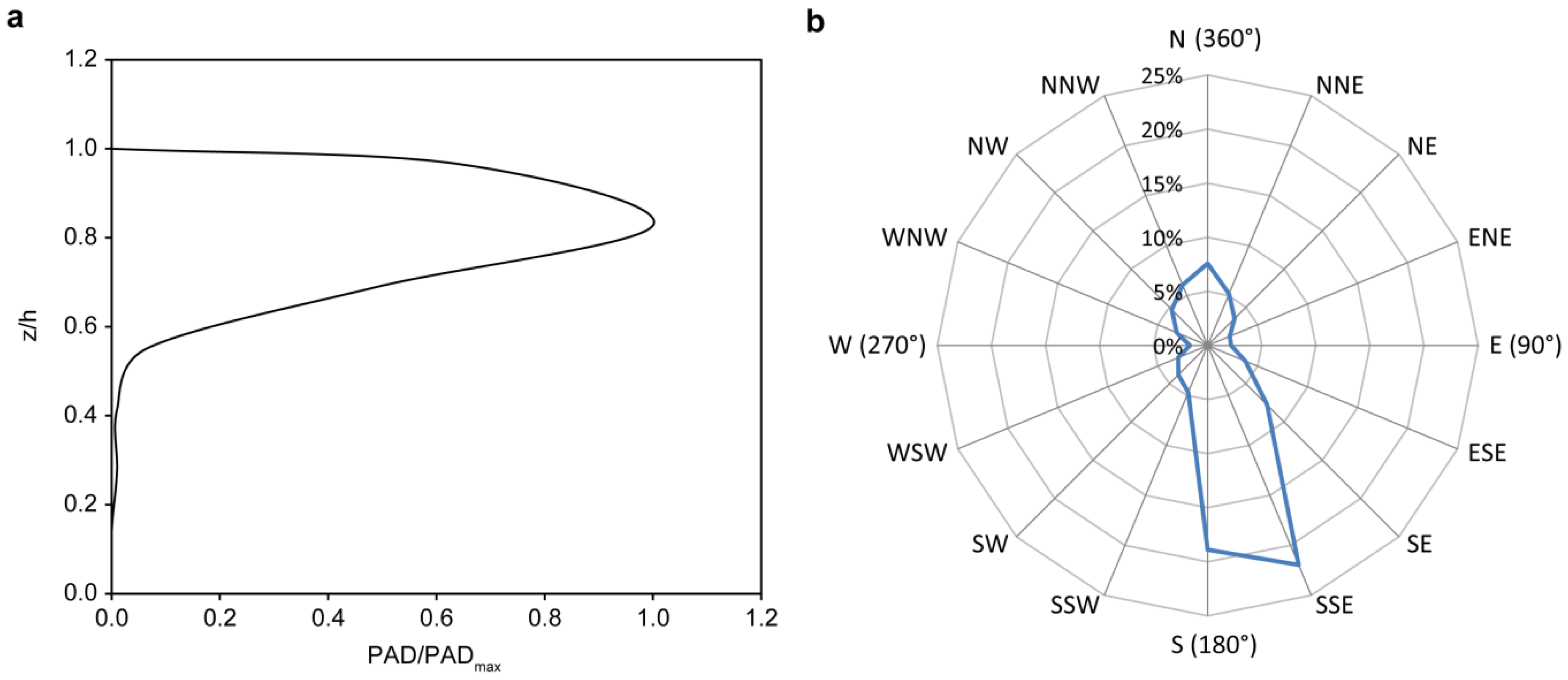
Air pressure fluctuations and airflow characteristics were measured at the forest research site Hartheim, operated by the Chair of Environmental Meteorology of the University of Freiburg. It is located approximately 25 km southwest of Freiburg in the flat southern Upper Rhine Valley (47°56′04″N, 7°36′02″E, 201 m above sea level). The forest at the research site is a single-layered plantation of Scots pines (Pinus sylvestris L.) and was established in the 1960s. The mean tree height ($h$) in the year 2016 was approximately 18 m, and the mean stand density was 580 trees·ha⁻¹. The mean plant area index is 1.5. Figure 1a shows the normalized plant area density (PAD, in m²·m⁻³) profile at the research site.

The research site has a lattice tower with a top height of 30 m. It is equipped with a large number of meteorological instruments, including psychrometers to measure dry-bulb and wet-bulb temperature, radiometers to measure the components of the radiation balance, and ultrasonic anemometers [43]. Soil temperature and soil moisture were measured at two locations next to the tower at a depth of −0.10 m with Aquaflex probes (Umweltanalytische Produkte GmbH, Ibbenbüren, Germany). Furthermore, a soil temperature (${\theta }_S$, in K) was measured with PT100 sensors at the depths −0.01 m (${\theta }_{S1}$), −0.03 m (${\theta }_{S2}$), −0.05 m (${\theta }_{S3}$), −0.10 m (${\theta }_{S4}$), −0.20 m (${\theta }_{S5}$), and −0.40 m (${\theta }_{S6}$). Soil heat flux was measured at two locations ($H{f}_1$ and $H{f}_2$, in W·m⁻²) near the tower at a depth of −0.03 m with heat flux plates (HFP01SC, Hukseflux, Delft, The Netherlands).

According to the World Reference Base (WRB) classification, the soil at the research site is classified as Haplic Regosol [44]. Its topsoil is covered by a humus type of mull followed by a silty loam texture over a subsoil consisting partly of sand and gravel [8].

2.2. Airflow Measurements

The wind vector components in $x$− ($u$), $y$− ($v$), and $z$− direction ($w$) were measured simultaneously (in m·s⁻¹) at five different heights with ultrasonic anemometers (81000VRE, R.M. Young Company, Traverse City, MI, USA) during the period 29 March 2016 to 13 July 2016. The ultrasonic anemometers were mounted on the tower at the heights 2 m ($z_1/h$ = 0.11), 9 m ($z_2/h$ = 0.50), 18 m ($z_3/h$ = 1.00), 21 m ($z_4/h$ = 1.15), and 30 m ($z_5/h$ = 1.67) above ground level (a.g.l.). The sampling rate of the ultrasonic anemometers was 10 Hz and data were analyzed per 30 min interval. At the measurement site, airflow from northern and southern directions dominated during the measurement period (Figure 1b). To minimize the influence of the tower on the measurements, all ultrasonic anemometers were installed on 1.5 m long supporting booms directed to the west. The maxima of the 30 min mean wind speed during the measurement period at $z_1$, $z_2$, $z_3$, $z_4$, and $z_5$ were ${\overline{U}}_{1,max}$ = 0.8 m·s⁻¹, ${\overline{U}}_{2,max}$ = 1.2 m·s⁻¹, ${\overline{U}}_{3,max}$ = 3.8 m·s⁻¹, ${\overline{U}}_{4,max}$ = 4.1 m·s⁻¹, and ${\overline{U}}_{5,max}$ = 6.5 m·s⁻¹.

2.3. Air Pressure Measurements

2.3.1. Pressure Sensors

Below-canopy and soil air pressures ($p$, in Pa) were measured with three piezo-resistive differential pressure sensors (GMSD 2.5 MR, Greisinger Electronic GmbH, Regenstauf, Germany) to achieve the highest accuracies currently available (sensitivity 0.1 Pa, accuracy 1%, measurement range −2 hPa to +2.5 hPa). Two sensors were installed at the same heights as the below-canopy airflow measurements ($p_1$ at $z_1$, $p_2$ at $z_2$). An additional pressure sensor measured the air pressure fluctuations in the soil ($p_0$ at $z_0$ = −0.03 m). The air pressure data were also analyzed per 30 min interval.

One inlet of each pressure sensor in the below-canopy space was connected with a tube (inner diameter: 2 mm) to a low-cost pressure head. The pressure head consists of a metal pipe (inner diameter: 2 mm) which was inserted half way into a plastic sphere with 25 holes (outer diameter: 72 mm, hole diameter: 9 mm). The sphere was used to ensure omnidirectionality of the air pressure measurement and to prevent errors due to dynamic pressure effects. The other inlet of the pressure sensor was connected to the reference, which filters all high-frequency air pressure fluctuations (see below).

This design was tested against a state-of-the-art high-performance DigiPort pressure head (DigiPort, Paroscientific Inc., Redmond, WA, USA) used for barometric air pressure measurements at high wind speeds [33]. The DigiPort pressure head has been designed to provide accuracy in air pressure measurements of 1 Pa at a wind speed of 5 m·s⁻¹ [45]. For all 30 min intervals with mean wind speeds up to 1.5 m·s⁻¹ the measurement values obtained from the DigiPort pressure head correlated well with the measurement values obtained from our pressure head (Pearson correlation coefficient $R$ = 0.99 ± 0.01). In the below-canopy space, 30 min mean values of the wind speed never exceeded 1.5 m·s⁻¹. Therefore, it was believed that the air pressure measurements below the forest canopy were not disturbed by dynamic pressure errors.

2.3.2. Pressure Reference

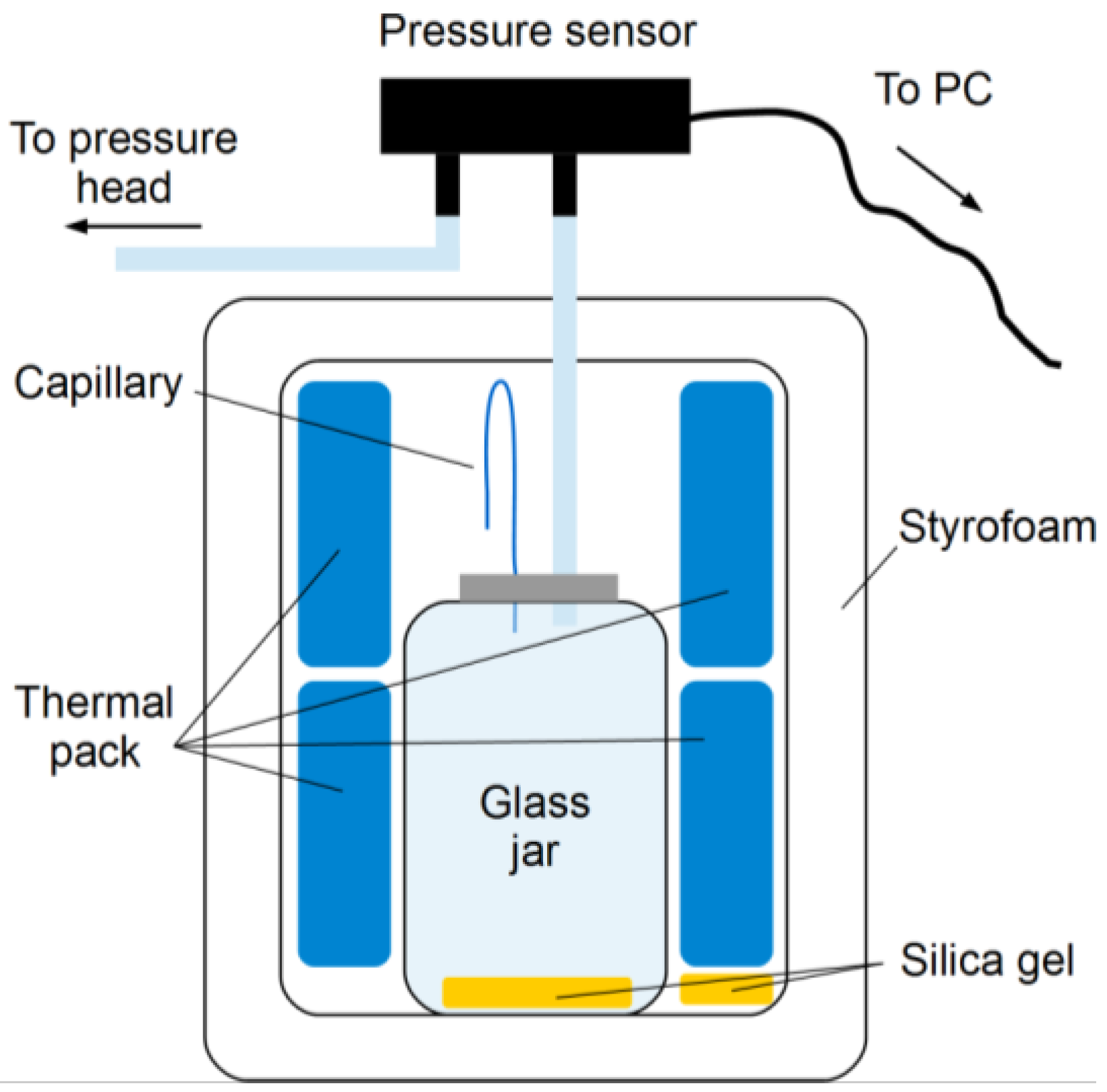
The pressure reference consists of two nested volumes: a glass jar (volume: 0.225 l inside an insulating box of Styrofoam (volume: 4.2 l) which is in exchange with the atmosphere (Figure 2). The inlet of the pressure sensor for the reference is connected to the glass jar. Air exchange between the glass jar and the Styrofoam box is possible through a capillary, which acts as a pressure equalizer. The capillary has a length $L=0.15\mathrm{m}$ and inner diameter $d=2,r=0.124\mathrm{mm}$, with $r$ being the radius of the capillary. To avoid temperature effects on the air pressure measurement, the temperature inside the reference chamber should only change slowly over time [37]. Therefore, thermal packs were put inside the box to increase thermal inertia, and the insulating box was wrapped in a reflecting blanket to minimize heating up due to insulation. In addition, silica gel inside the box was used to maintain a low humidity and to avoid blocking the capillary with water droplets.

The high-frequency cutoff of the pressure reference was determined theoretically as follows. The volumetric flux $q_v$ of air (in m³·s⁻¹) with dynamic viscosity $\eta$ (in kg·m⁻¹·s⁻¹) through the capillary caused by the difference between the air pressure in the reference chamber $p_c$ (in Pa) and the air pressure of the atmosphere $p_a$ (in Pa) is [46]:

$$q_v=\frac{\pi }{8}\frac{r^4}{\eta L}\left(p_c-p_a\right)$$

(1)

With the ideal gas law, constant $V$ (in m³), and assuming constant air temperature ${\theta }_a$ (in K), the resulting change of amount of substance $dn$ (in mol) in the chamber per change of time $dt\prime$ can be written as:

$$\frac{dn}{dt\prime }=\frac{V}{R_g{\theta }_a}\frac{d{p}_c}{dt\prime }$$

(2)

The universal gas constant is $R_g=8.3144598\mathrm{J}\cdot {\mathrm{mol}}^{-1}\cdot {\mathrm{K}}^{-1}$ [47]. With the molar volume of air $V_m$ (in m³·mol⁻¹) Equations (1) and (2) can be equated:

$$\frac{dn}{dt\prime }{V}_m=-q_v$$

(3)

$$\frac{V{V}_m}{R_g{\theta }_a}\frac{d{p}_c}{dt\prime }=-\frac{\pi }{8}\frac{r^4}{\eta L}\left(p_c-p_a\right)$$

(4)

Solving this differential equation from time $t_0=0$ to time $t$ with $p_c\left(0\right)=p_0$ and $p_c\left(t\right)=p_t$ yields:

$$p_t=p_a+\left(p_0-p_a\right)e^{-\beta t}$$

(5)

$$\beta =\frac{\pi }{8}\frac{r^4{R}_g{\theta }_a}{\eta LV{V}_m}$$

(6)

The time $\tau$ (in s), when the difference between the air pressure in the reference chamber and the air pressure outside has been attenuated to $1/e$ times the initial value is:

$$\tau =\frac{1}{\beta }$$

(7)

The time constant $\tau$ along with the values for $\eta$ and $V_m$ used for the calculation are listed in

Table 1. Values for $\eta$ and calculated $V_m$ and $\tau$ (time constant) of air for $T=298\mathrm{K}$ (25 °C) and $p=1013.25\mathrm{hPa}$.

Quantity	Value
Dynamic viscosity $\eta$	$18.468\times {10}^{-6}$kg·m−1·s−1 [48]
Molar volume $V_m$	$24.453\times {10}^{-3}$m3·mol−1
$\tau$	$933.7$ s

.

After a time of $3\tau$, the pressure difference between the reference chamber and the outside was smaller than 5% of the initial value. This value was used to calculate the frequency cutoff $f_c$. Thus, the reference acts as a low-pass filter with $f_c=1/3\tau \approx 4\times {10}^{-4}$ Hz. The filter behavior was verified by evaluating the quotient of the Fourier spectral energy density of the filtered pressure signal and the Fourier spectral energy density of the unfiltered pressure signal. The resulting filter behavior yielded a cutoff frequency of $5\times {10}^{-4}$ Hz, i.e., about 33 min, and was therefore in good agreement with the theoretical considerations.

2.4. Soil Gas Measurements

To investigate the effect of air pressure fluctuations on soil gas concentration, a state-of-the-art gas concentration measurement system was used [49]. The measurement system consists of a gas sampling pole, a tracer gas injection device, a valve system and a microgas chromatograph (3000 Micro GC Gas 176 Analyzer, Inficon GmbH, Cologne, Germany). The gas sampling pole has a length of 50 cm and features gas sampling membranes at seven depths (from +0.01 m to −0.41 m depth). At a soil depth of −0.21 m, a tracer gas was continuously injected. In this study, helium was used as tracer gas, since it is inert and has a low solubility in water [49]. The soil air was sampled through the membranes at several depths and transferred to the microgas chromatograph, which analyzed the soil air and determined the helium concentration. Thus, the helium concentration profile could be monitored. Assuming molecular diffusion as the main soil gas transport process, a steady-state profile of helium concentration is reached. A deviation of the soil helium profile from the steady-state profile indicated an external effect on soil gas transport.

The gas sampling pole was installed approximately 10 m southwest of the tower in a hole drilled in the soil. Helium was continuously injected at a constant rate into the soil during the period 5 July 2016 to 13 July 2016. Helium concentrations (He, in ppm) were measured at the five depths of −0.01 m ($H{e}_1$), −0.06 m ($H{e}_2$), −0.11 m ($H{e}_3$), −0.31 m ($H{e}_4$), and −0.41 m ($H{e}_5$), and the helium concentrations measured at −0.01 m were used to study the effect of air pressure fluctuations on topsoil gas concentrations.

2.5. Data Processing

2.5.1. Airflow Data

The half-hourly time series of wind vector data were despiked and a double rotation was applied [50]. In addition, the data of heights $z_1$–$z_4$ were rotated in the mean wind direction at $z_5$, ensuring that for the time series of all heights the same coordinate system was used. Data of 30 min intervals when wind from eastern directions prevailed were excluded from the analysis (<10% of all 30 min intervals) to rule out influences from the measurement tower.

To distinguish between different atmospheric stabilities, the Obukhov length $\Lambda$ (in m) was calculated [51,52]:

$$\Lambda =\frac{-\overline{{\theta }_v}{u}_{*}^3}{\kappa g\overline{w^{\prime }{\theta }_v^{\prime }}}$$

(8)

with the virtual potential temperature ${\theta }_v$ (in K), the friction velocity $u_{*}={\left|{\overline{u^{\prime }{w}^{\prime }}}^2+{\overline{v^{\prime }{w}^{\prime }}}^2\right|}^{1/4}$ (in m·s⁻¹), the von Kármán constant $\kappa$ = 0.4 and the gravitational acceleration $g$ = 9.81 m·s⁻¹. The canopy-top stability parameter ${\zeta }_3=z_3/{\Lambda }_{z_3}$ was calculated for every 30 min interval [50]. All available half-hourly data sets were then assigned to the six stability classes listed in

Table 2. Classification of atmospheric stability according to the stability parameter ${\zeta }_3$.

Stability Class	${\mathit{\zeta }}_3$
Very stable	>1
Stable	0.6 … 1
Transition to stable	0.02 … 0.6
Near-neutral	−0.03 … 0.02
Forced convection	−0.8 … −0.03
Free convection	<−0.8

.

For every 30 min interval the mean wind speed at canopy height (${\overline{U}}_3$) and the friction velocity at canopy height ($u_{*3}$) were calculated.

Five exchange regimes (C1 − C5) were defined based on the correlation of coherent structures derived from momentum flux analysis over all measurement heights [50]. Exchange regime C1 is associated with uncoupled momentum flux above and below the forest canopy, while exchange regime C5 is associated with fully coupled momentum flux from $z_5$ to $z_1$. That means, during times specified as C1, no momentum is transferred from $z_5$ downwards. On the other hand, during times specified as C5, momentum is transferred from $z_5$ down to the forest floor at $z_1$ [50].

2.5.2. Air Pressure Data

All pressure sensors were sampled with a rate of 2.0 Hz. Every 30 min interval influenced by precipitation were excluded from analysis. For each remaining interval the air pressure fluctuations were investigated separately for three different frequency ranges: high frequency range ($p_{\mathrm{high}}$, 0.1 Hz – 1.0 Hz), medium frequency range ($p_{\mathrm{med}}$, 0.01 Hz – 0.1 Hz) and low frequency range ($p_{\mathrm{low}}$, 0.001 Hz – 0.01 Hz). A fourth-order infinite impulse response (IIR) filter was used as a band-pass filter to separate the air pressure signal into separate frequency ranges. The air pressure fluctuations were described statistically by calculating the arithmetic means $\overline{p}$ and standard deviations ${\sigma }_p$.

Mean amplitudes of the air pressure fluctuations were determined through the upper envelope $p_{\max }$ and lower envelope $p_{\min }$ of the air pressure fluctuations: the mean peak-to-peak amplitude was defined as $\widehat{p}=\overline{p_{\max }-p_{\min }}$.

The dominating periods of the air pressure fluctuations $T$ (in s) per 30 min interval were determined by investigating the normalized wavelet variance spectrum [53,54,55]. The wavelet coefficients were calculated for 100 scales using the Morlet wavelet, corresponding to up to 103 s. Then, the normalized wavelet variance spectrum was calculated. The scale $a$ of the first peak in the spectrum is associated with the dominating wavelet scale of the air pressure fluctuations. The Fourier-equivalent frequency $F_a$ (in Hz) of a wavelet scale $a$ can be calculated from the center frequency $F_c$ of the used wavelet (in cycles per unit time) and the sampling period $t_s$ (in s) [56]:

$$F_a=\frac{F_c}{a{t}_s}$$

(9)

Thus, the dominating period is $T=1/F_a$.

The correlation and time lags between two air pressure datasets $i$ and $j$ was determined by calculating the Pearson correlation coefficient $R\left(p_i,p_j\right)$ and the cross-correlation between $p_i$ and $p_j$. The Wilcoxon rank sum (WRS) test was used to evaluate if differences between air pressure fluctuation properties for different stability conditions and different exchange regimes were significant (level of significance $\alpha$ = 0.05) [57].

To describe the strength of the air pressure fluctuations, the pumping coefficient $\gamma$ (in Pa·s⁻¹) was defined as follows. First, the absolute slope $\left|\mathsf{∆}p/\mathsf{∆}t\right|$ (with $\mathsf{∆}t=1/F_s$ = 0.5 s) between two subsequent measurement points is calculated for every measurement point in the 30 min interval. Then, $\gamma$ was obtained by calculating the mean of all absolute slopes in the 30 min interval:

$$\gamma =\overline{\left|\frac{\mathsf{∆}p}{\mathsf{∆}t}\right|}$$

(10)

Therefore, the pumping coefficient $\gamma$ describes the mean change in air pressure fluctuation amplitude per second in a 30 min interval.

3. Empirical Modeling of Topsoil Helium Concentrations

To identify the factors that have an effect on the temporal evolution of $H{e}_1$, the ensemble learning method random forests (RF) implemented in the Matlab^® Statistics and Machine Learning Toolbox (The MathWorks Inc., Natick, MA, USA, Release 2016a) was applied. Using bootstrap samples, RF combined binary decision trees, which were built on 66% of the available helium concentration data (D1). The remaining 34% of the helium concentration data (D2) were used for model evaluation and prediction of the topsoil helium concentration.

The following predictor variables were considered as potentially informative input to the RF model: dry-bulb and wet-bulb air temperature above and below the canopy, components of the radiation balance at canopy top, soil temperatures, soil moistures, and soil heat fluxes.

Prior to model building, (1) all variables were detrended using a sixth degree polynomial; and (2) the strength of collinearity among the predictor variables was assessed by the variance inflation factor ($VIF<2$) and Belsley collinearity diagnostics [58]. If collinearity was detected among two predictor variables, the predictor variable contributing less to the final RF model accuracy was excluded from further model building. The relative contribution of the selected predictor variables to the final RF model output was evaluated by the predictor importance (PI, in %) quantified for D2. The PI values were used to identify important predictor variables which strongly impact the RF model accuracy after being randomly permuted.

After testing for collinearity, various combinations of predictor variables were evaluated for their power to predict $H{e}_1$. Starting with one predictor variable, further predictor variables were sequentially added to the RF model and retained when the model error decreased. The coefficient of determination $\left(R^2\right)$, the mean squared error $\left(MSE\right)$ and the mean absolute error ($MAE$) were used to assess the accuracy with which the RF model simulated the measured $H{e}_1$ concentration values.

4. Results and Discussion

4.1. Frequency Characteristics of Air Pressure Fluctuations

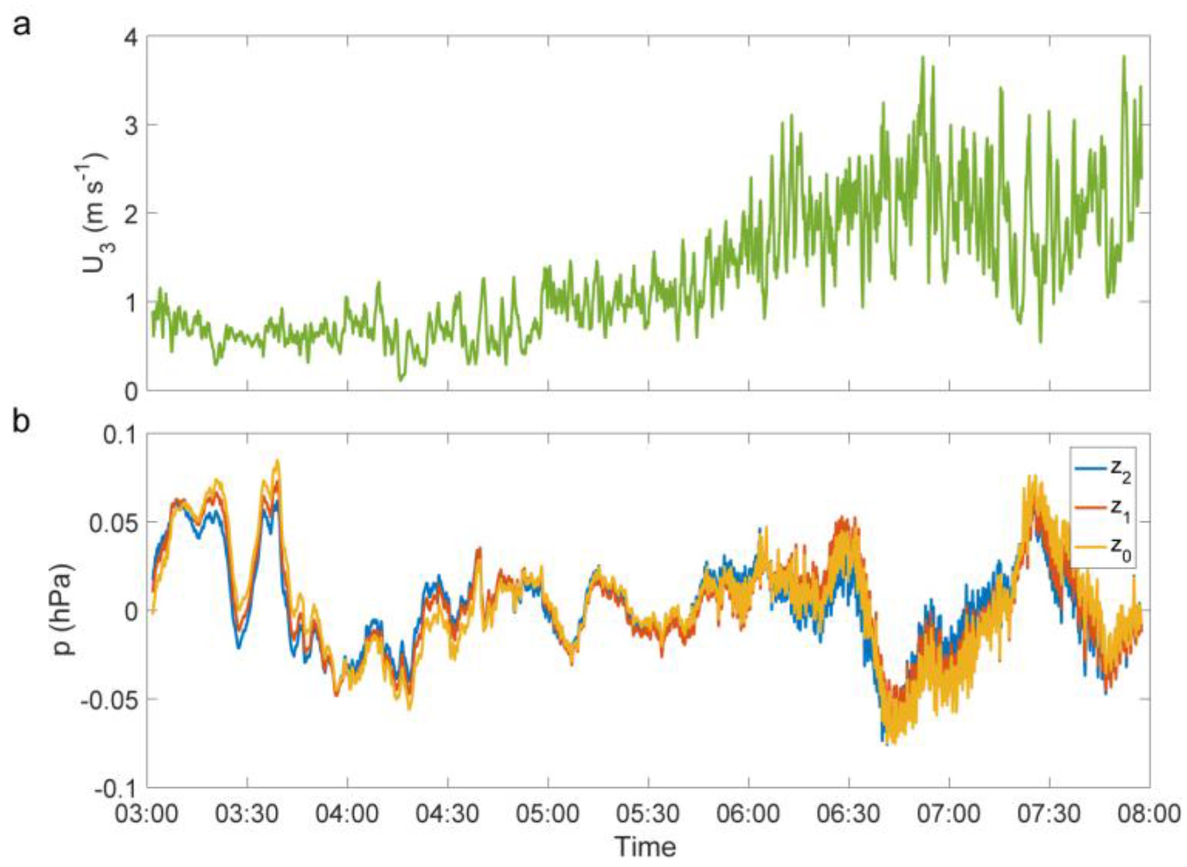
Figure 3 shows the raw air pressure signals measured below the canopy ($p_1$ and $p_2$) and in the soil ($p_0$) over a six-hour period (22 April 2016, 02:00–08:00) with increasing above-canopy wind speed $U_3$. The low-frequency fluctuations are visible in the air pressure signals of all measurement heights. However, as $U_3$ increases, the air pressure signals contain fluctuations of higher frequencies that do not occur at low $U_3$ values. Other than results from a previous study [39], the fluctuations did not show a deterministic relationship with $U$, $u$, $v$, $w$, momentum flux ($u\prime w\prime$), or air temperature (${\theta }_a$) associated with coherent structures [59]. Therefore, subsequent analysis focuses on 30 min statistics.

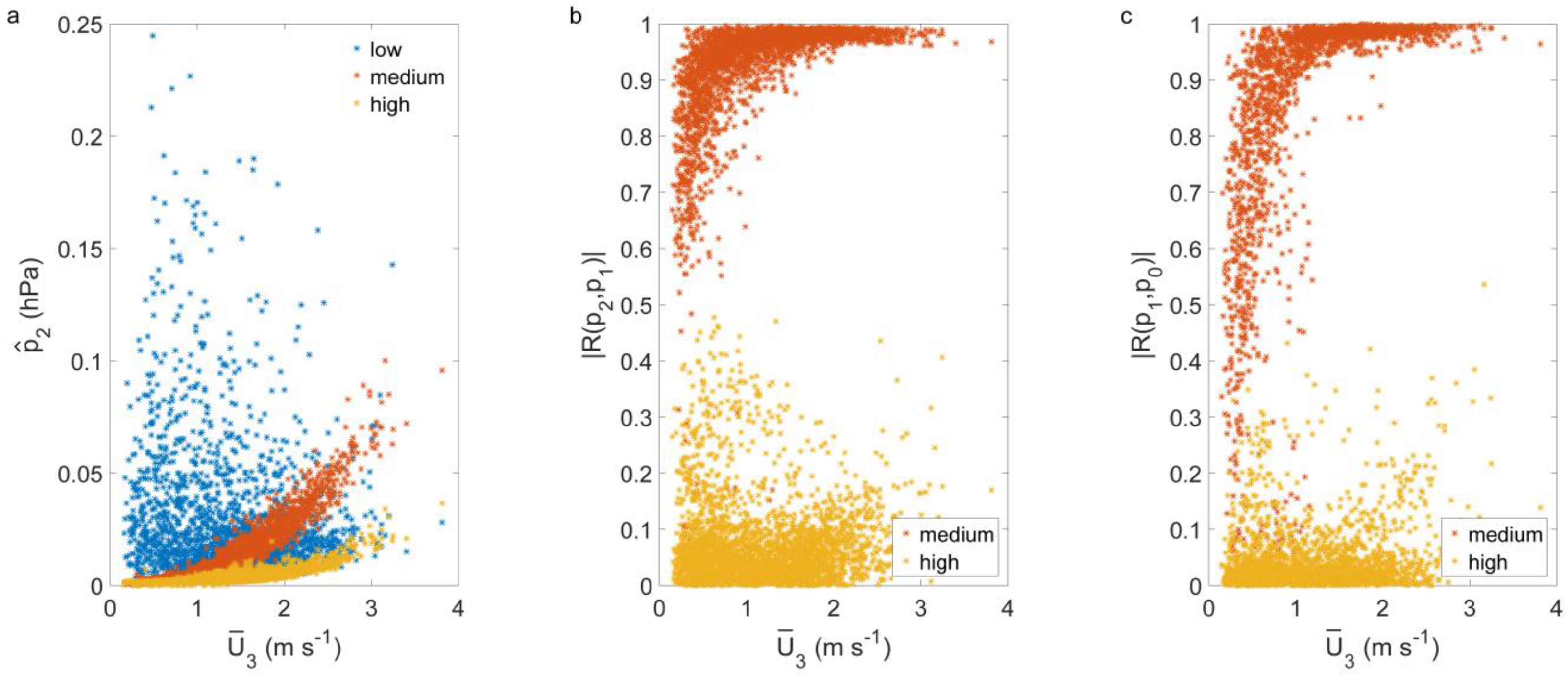
The dependence of the air pressure amplitudes at $z_2$ (${\widehat{p}}_2$) on above-canopy mean wind speed (${\overline{U}}_3$) was used to determine whether the amplitudes of the fluctuations in a frequency range change as a function of wind speed (Figure 4a). In addition, the correlation of the fluctuations between $p_2$ and $p_1$, and $p_1$ and $p_0$ was determined by analysis of $R\left(p_2,p_1\right)$ and $R\left(p_1,p_0\right)$ with respect to ${\overline{U}}_3$ (Figure 4b). Combination of both information yielded the frequency range of interest. While no clear dependence of the mean amplitudes of the low frequency air pressure fluctuations (${\widehat{p}}_{2,\mathrm{low}}$) on mean above-canopy wind speed was found, ${\widehat{p}}_2$ increased with increasing ${\overline{U}}_3$ in the medium and high frequency range (Figure 4a). Therefore, low frequency fluctuations were contained in the air pressure signal independent of wind speed, and were not investigated further. The fluctuations in the medium frequency range (0.01 Hz – 0.1 Hz) showed strong correlation below the canopy, while the high frequency fluctuations were mostly uncorrelated (Figure 4b,c). Moreover, the amplitudes of the air pressure fluctuations in the medium frequency range (${\widehat{p}}_{2,\mathrm{med}}$) were around five times larger than the amplitudes of the air pressure fluctuations in the high frequency range (${\widehat{p}}_{2,\mathrm{high}}$). Based on these results, subsequent analysis of air pressure fluctuations focuses on the medium frequency range. This result is also in agreement with a previous study that suggested air pressure fluctuations with frequencies <0.1 Hz are important [12].

4.2. Dependences on Airflow Characteristics

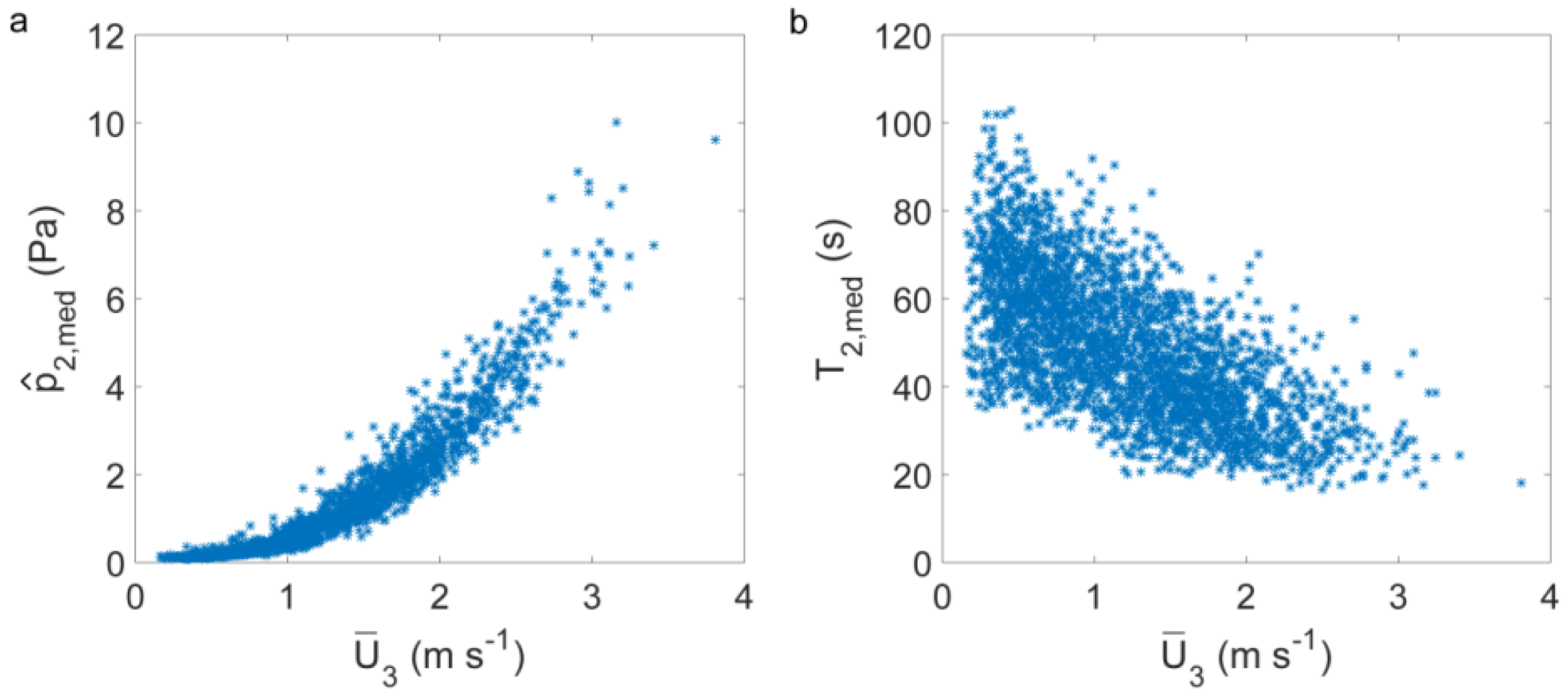
4.2.1. Mean Wind Speed at Canopy Height

Since strongly correlated air pressure fluctuations were measured at $z_2$ to $z_0$, dependences are only shown for one air pressure signal ($p_2$). While no clear dependence of ${\sigma }_{p_{2,\mathrm{med}}}$ on the mean wind speed measured at the same height ${\overline{U}}_2$ was found (Figure 5a), ${\sigma }_{p_{2,\mathrm{med}}}$ showed a quadratic dependence on ${\overline{U}}_3$ (Figure 5b) in accordance with a previous study [7]. This emphasizes that these air pressure fluctuations are not produced locally. In contrast to other studies, no clear linear dependence of ${\sigma }_p^2$ on the mean wind speed $\overline{U}$ [5,6], or an exponential dependence of ${\sigma }_p$ on the friction velocity $u_{*}$ [8] was found.

The threshold value of ${\overline{U}}_3$ for the occurrence of air pressure fluctuations in the below-canopy space in the medium frequency range can be specified as approximately 1.5 m·s⁻¹, which is also consistent with results from Fourier spectral analysis. Fourier spectra of 30 min intervals with ${\overline{U}}_3$ < 1.5 m·s⁻¹ have a slope of −1 in the medium-frequency range. During intervals with ${\overline{U}}_3$ > 1.5 m·s⁻¹ a broad peak forms between 0.01 Hz and 0.1 Hz.

A similar dependence on ${\overline{U}}_3$ was found for the amplitudes ${\widehat{p}}_{2,\mathrm{med}}$ (Figure 6a). Moreover, a decrease of $T_{2,\mathrm{med}}$ with increasing ${\overline{U}}_3$ was found (Figure 6b). At the highest values of ${\overline{U}}_3$, the values decreased to 20 s. Results from WRS test showed that ${\widehat{p}}_{\mathrm{med}}$ increased significantly with increasing ${\overline{U}}_3$, but that there were no significant differences between ${\widehat{p}}_{\mathrm{med}}$ at $z_2$, $z_1$ and $z_0$. Moreover, results from WRS test also showed a significant decrease of mean periods $T_{\mathrm{med}}$ with increasing ${\overline{U}}_3$.

4.2.2. Atmospheric Stability

The dependence of the amplitudes ${\widehat{p}}_{\mathrm{med}}$ and periods $T_{\mathrm{med}}$ was analyzed under different stability conditions (

Table 3. Mean values for mean above-canopy wind speed ${\overline{U}}_3$, dominant period in the medium frequency range $T_{\mathrm{med}}$ and amplitudes in the medium frequency range ${\widehat{p}}_{\mathrm{med}}$ under different stability conditions.

Stability	${\overline{\mathit{U}}}_3$ (m·s−1)	${\mathit{T}}_{\mathbf{m}\mathbf{e}\mathbf{d}}$ (s)			${\widehat{\mathit{p}}}_{\mathbf{m}\mathbf{e}\mathbf{d}}$ (Pa)
		${\mathit{z}}_0$	${\mathit{z}}_1$	${\mathit{z}}_2$	${\mathit{z}}_0$	${\mathit{z}}_1$	${\mathit{z}}_2$
Very stable	0.6 ± 0.3	59 ± 13	60 ± 14	55 ± 15	0.3 ± 0.3	0.3 ± 0.3	0.4 ± 0.4
Stable	1.0 ± 0.4	55 ± 14	55 ± 14	52 ± 14	0.7 ± 0.5	0.7 ± 0.5	0.7 ± 0.6
Transition to stable	1.6 ± 0.5	43 ± 13	45 ± 13	41 ± 13	1.9 ± 1.3	1.8 ± 1.3	1.9 ± 1.4
Near neutral	2.0 ± 0.5	38 ± 10	39 ± 10	35 ± 10	2.9 ± 1.8	2.8 ± 1.7	3.0 ± 1.9
Forced convection	1.6 ± 0.5	44 ± 12	46 ± 13	41 ±13	2.0 ± 1.3	1.8 ± 1.4	2.0 ± 1.5
Free convection	0.9 ± 0.4	54 ± 14	56 ± 14	51 ± 16	0.9 ± 0.8	0.7 ± 0.7	0.8 ± 0.9

). Results from the WRS test showed that ${\widehat{p}}_{\mathrm{med}}$ was significantly larger under near-neutral conditions than ${\widehat{p}}_{\mathrm{med}}$ under all other stability conditions. This can be attributed to higher wind speeds under near-neutral conditions, which are assumed to be the main generator of the air pressure fluctuations.

4.2.3. Exchange Regime

Since dependences of ${\sigma }_p$ on $u_{*}$ had been found in previous studies [19], and $u_{*}$ is related to $u\prime w\prime$, a dependence of $p$ on $u\prime w\prime$ was expected. In addition, $p/\rho$ ($\rho$: volumetric mass density) and $u\prime w\prime$ have the same unit. Therefore, differences between the air pressure fluctuations under the momentum flux-derived exchange regimes C1 (no coupling, 83% of all 30 min intervals) and C5 (completely coupled, 12% of all 30 min intervals) were investigated.

Table 4. Mean values for mean above-canopy wind speed ${\overline{U}}_3$, dominant period in the medium frequency range $T_{\mathrm{med}}$ and amplitudes in the medium frequency range ${\widehat{p}}_{\mathrm{med}}$ under different exchange regimes.

Exchange Regime	${\overline{\mathit{U}}}_3$ (m·s−1)	${\mathit{T}}_{\mathbf{m}\mathbf{e}\mathbf{d}}$ (s)			${\widehat{\mathit{p}}}_{\mathbf{m}\mathbf{e}\mathbf{d}}$ (Pa)
		${\mathit{z}}_0$	${\mathit{z}}_1$	${\mathit{z}}_2$	${\mathit{z}}_0$	${\mathit{z}}_1$	${\mathit{z}}_2$
C1	1.2 ± 0.7	47 ± 14	49 ± 15	45 ± 15	1.7± 1.4	1.4 ± 1.4	1.5 ± 1.5
C5	1.1 ± 0.5	52 ± 14	54 ± 14	49 ± 15	1.1 ± 0.7	1.0 ± 0.7	1.1 ± 0.8

lists the means for $T_{\mathrm{med}}$ and ${\widehat{p}}_{\mathrm{med}}$ under the different exchange regimes.

Results from WRS test showed no significant differences between the two exchange regimes. Since mean values for ${\overline{U}}_3$ under C1 and C5 are similar, these results emphasize that the occurrence of air pressure fluctuations in the medium frequency range are dependent on ${\overline{U}}_3$.

4.3. Pressure-Pumping Coefficient

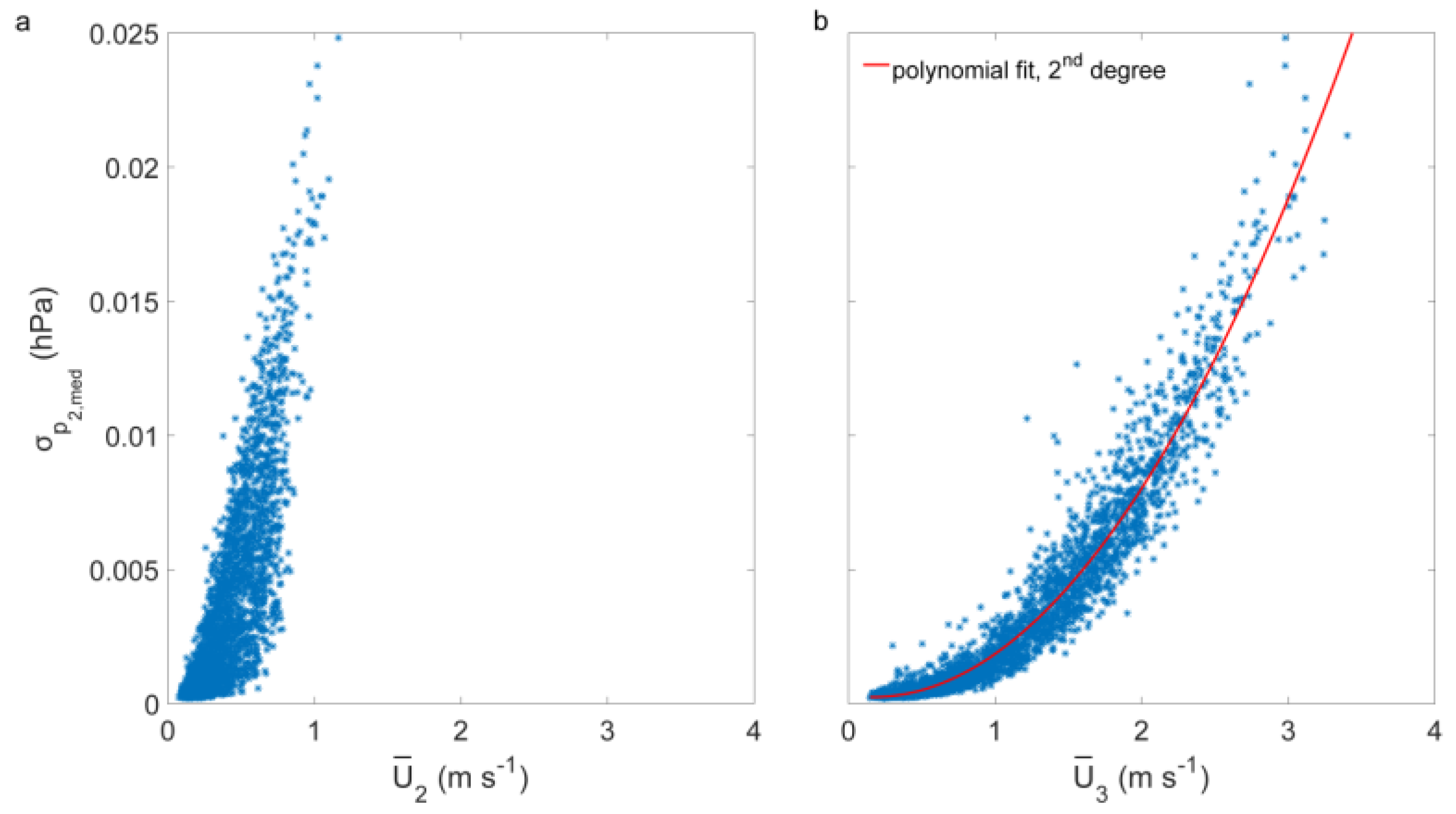
Since pressure pumping is especially important for soil gas transport, the dependence of the pressure-pumping coefficient in the soil (${\gamma }_{0,\mathrm{med}}$) on the mean above-canopy wind speed ${\overline{U}}_3$ was investigated. Values of ${\gamma }_{0,\mathrm{med}}$ vary between 0 during intervals of low ${\overline{U}}_3$ and 0.44 Pa·s⁻¹ during intervals of high ${\overline{U}}_3$ (Figure 7).

Results from WRS test showed a significant increase of ${\gamma }_{0,\mathrm{med}}$ with increasing ${\overline{U}}_3$. The dependence of ${\gamma }_{0,\mathrm{med}}$ on ${\overline{U}}_3$ for ${\overline{U}}_3$ > 0.75 m·s⁻¹ can be described by a second-degree polynomial ($R^2$ = 0.97)

$${\gamma }_{0,\mathrm{med}}=0.0451{{\overline{U}}_3}^2-0.05527{\overline{U}}_3+0.02370$$

(11)

In contrast, the pressure-pumping coefficient calculated for the low-frequency range ${\gamma }_{0,\mathrm{low}}$ remained relatively constant, varying between 0.008 ± 0.004 Pa·s⁻¹ at ${\overline{U}}_3$ < 0.5 m·s⁻¹ and 0.030 ± 0.012 Pa·s⁻¹ at ${\overline{U}}_3$ > 2.5 m·s⁻¹. The pressure-pumping coefficient for the high-frequency range ${\gamma }_{0,\mathrm{high}}$ also stayed constant with ${\overline{U}}_3$, but was on average 4.5 times larger than ${\gamma }_{0,\mathrm{low}}$. It varied between 0.042 ± 0.004 Pa·s⁻¹ at ${\overline{U}}_3$ < 0.5 m·s⁻¹ and 0.070 ± 0.010 Pa·s⁻¹ at ${\overline{U}}_3$ > 2.5 m·s⁻¹. Therefore, ${\gamma }_{0,\mathrm{med}}$ is by far the most important pressure-pumping coefficient.

The threshold value of ${\overline{U}}_3$ = 1.5 m·s⁻¹ for the occurrence of air pressure fluctuations in the medium-frequency range is also a reasonable threshold value for pressure pumping in the soil for this measurement site.

4.4. Influence on Soil Gas Transport

The mean helium concentration at the injection depth for the period 5 July 2016 to 13 July 2016 $(\langle H{e}_3\rangle )$ was 388 ± 69 ppm. Towards the soil surface, the mean helium concentration decreased to $\langle H{e}_2\rangle$ = 115 ± 11 ppm and $\langle H{e}_1\rangle$ = 28 ± 5 ppm.

The evaluation of collinearity among the most important predictor variables revealed that ${\overline{U}}_3$ and ${\gamma }_{0,\mathrm{med}}$, and ${\overline{U}}_3$ and $H{f}_{mean}$ (mean of $H{f}_1$ and $H{f}_2$) were collinear $(VIF>3.5)$ while ${\gamma }_{0,\mathrm{med}}$ did not exhibit any collinearity with other important predictor variables. Therefore, ${\overline{U}}_3$ was excluded from building the final RF model.

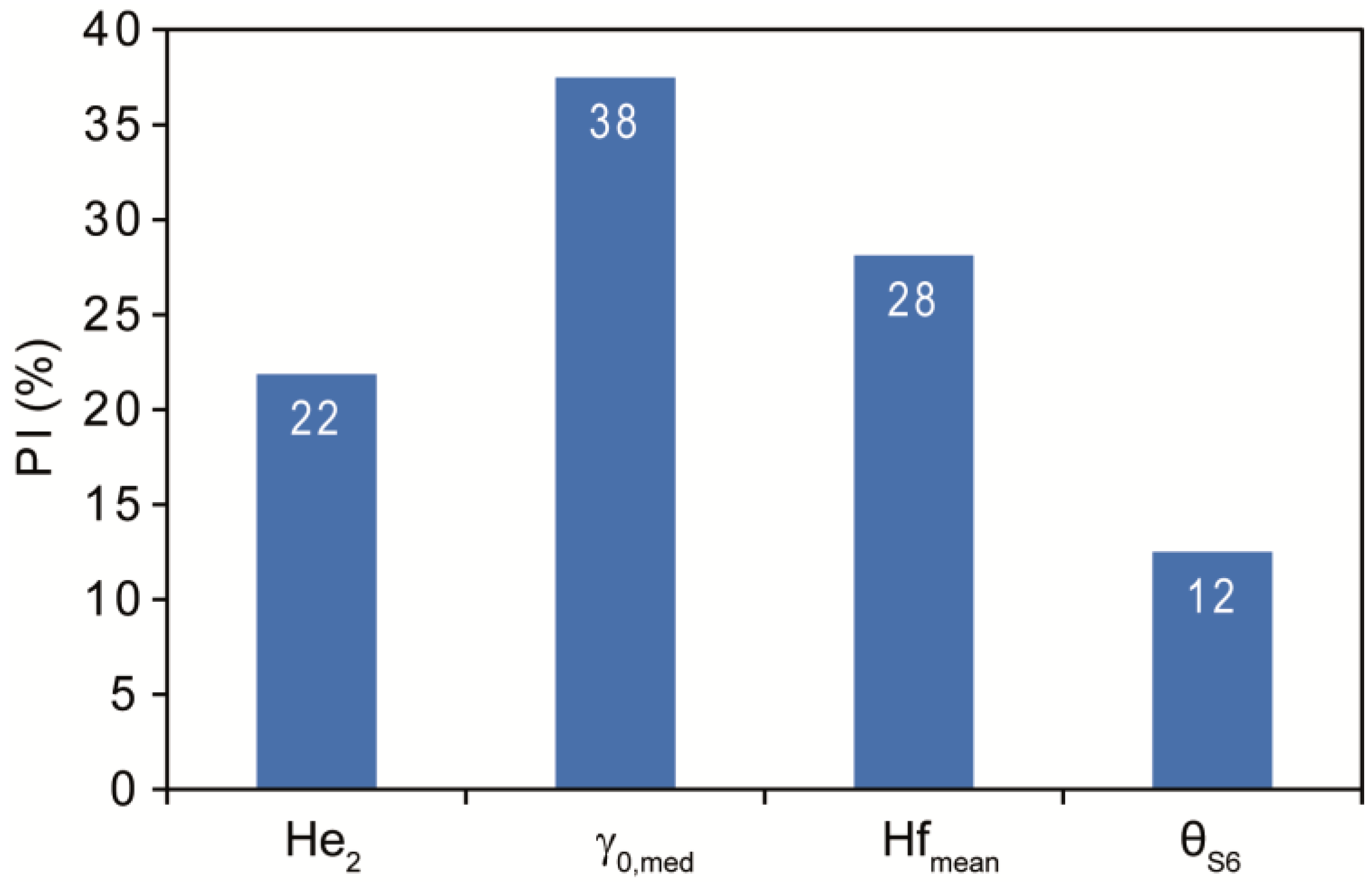
The predictor variable combination that provided the best discrimination between RF modeling results for D2 data and $H{e}_1$ $\left(R^2=0.72\right)$ included $H{e}_2$, ${\gamma }_{0,\mathrm{med}}$, $H{f}_{mean}$, and ${\theta }_{S6}$. Results from PI evaluation demonstrate that the relative impact of ${\gamma }_{0,\mathrm{med}}$ on the predictive accuracy of the RF model was greatest $\left(PI=38\%\right)$.

The second most important predictor variable was $H{f}_{mean}\left(PI=28\%\right)$, followed by $H{e}_2\left(PI=22\%\right),$ and ${\theta }_{S6}\left(PI=12\%\right)$ (Figure 8). Considering the results from the collinearity analysis, the most accurate RF model including ${\overline{U}}_3$ as a predictor variable yielded $R^2=0.64$. This finding indicates that ${\gamma }_{0,\mathrm{med}}$ is better suited for empirical modelling of $H{e}_1$ than ${\overline{U}}_3$.

The RF model results indicate that large proportions of $H{e}_1$ variance can be explained by at least two processes. On the one hand, $H{e}_1$ variance is strongly affected by the soil heat flux. On the other hand, a substantial proportion of $H{e}_1$ variance can be explained by wind-induced air pressure fluctuations.

5. Conclusions

The results of the present study reveal a strong positive, quadratic relationship between 30 min mean values of wind speed at canopy top and pressure-pumping coefficient in the topsoil. This simplifies the quantification of the pressure-pumping effect considerably, since only wind speed has to be measured. However, it is still unclear whether this relationship is site-dependent or universally applicable. The pressure pumping may be affected by the canopy type, canopy height, and foliage. Therefore, the presented methodology has to be conducted at other sites with different canopy characteristics in the future.

The pressure-pumping coefficient was calculated based on air pressure fluctuations occurring in the frequency range 0.01 Hz – 0.1 Hz. It is a measure for the half-hourly intensity of air pressure fluctuations and describes the mean change in pressure per second. Empirical modeling of helium concentration demonstrated that the pressure-pumping coefficient is an important predictor for changes in the topsoil gas concentration, and thus, an important factor for soil gas transport.

Knowledge of the half-hourly amplitudes and frequencies of the air pressure fluctuations can serve as a basis for the investigation of the pressure-pumping effect in the laboratory. By reproducing air pressure fluctuations based on the findings of this study, laboratory studies allow for a clear quantification of air pressure fluctuations on topsoil gas concentrations.

References

- Gossard, E.E. Spectra of atmospheric scalars. J. Geophys. Res. 1960, 65, 3339–3351. [Google Scholar] [CrossRef]
- Kimball, B.A.; Lemon, E.R. Spectra of air pressure fluctuations at the soil surface. J. Geophys. Res. 1970, 75, 6771–6777. [Google Scholar] [CrossRef]
- Elliott, J.A. Microscale pressure fluctuations near waves being generated by the wind. J. Fluid Mech. 1972, 53, 351–383. [Google Scholar] [CrossRef]
- Elliott, J.A. Microscale pressure fluctuations measured within the lower atmospheric boundary layer. J. Fluid Mech. 1972, 54, 427–448. [Google Scholar] [CrossRef]
- Sigmon, J.T.; Knoerr, K.R.; Shaughnessy, E.J. Microscale pressure fluctuations in a mature deciduous forest. Bound.-Layer Meteorol. 1983, 27, 345–358. [Google Scholar] [CrossRef]
- Sigmon, J.T.; Knoerr, K.R.; Shaughnessy, E.J. Leaf emergence and flow-through effects on mean winds peed profiles and microscale pressure fluctuations in a deciduous forest. Agric. For. Meteorol. 1984, 31, 329–337. [Google Scholar] [CrossRef]
- Shaw, R.H.; Paw, K.T.U.; Zhang, X.J.; Gao, W.; den Hartog, G.; Neumann, H.H. Retrieval of turbulent pressure fluctuations at the ground surface beneath a forest. Bound.-Layer Meteorol. 1990, 50, 319–338. [Google Scholar] [CrossRef]
- Maier, M.; Schack-Kirchner, H.; Hildebrand, E.E.; Holst, J. Pore-space CO2 dynamics in a deep, well-aerated soil. Eur. J. Soil Sci. 2010, 61, 877–887. [Google Scholar] [CrossRef]
- Farrell, D.A.; Greacen, E.L.; Gurr, C.G. Vapor transfer in soil due to air turbulence. Soil Sci. 1966, 102, 305–313. [Google Scholar] [CrossRef]
- Scotter, D.R.; Raats, P.A.C. Dispersion of water vapor in soil due to air turbulence. Soil Sci. 1969, 108, 170–176. [Google Scholar] [CrossRef]
- Clements, W.E.; Wilkening, M.H. Atmospheric pressure effects on 222Rn Transport across the earth-air interface. J. Geophys. Res. 1974, 79, 5025–5029. [Google Scholar] [CrossRef]
- Massman, W.J.; Sommerfeld, R.A.; Mosier, A.R.; Zeller, K.F.; Hehen, T.J.; Rochelle, S.G. A model investigation of turbulence driven pressure-pumping effects on the rate of diffusion of CO2, N2O, and CH4 through layered snowpacks. J. Geophys. Res. 1997, 102, 18851–18863. [Google Scholar] [CrossRef]
- Takle, E.S.; Massman, W.J.; Brandle, J.R.; Schmidt, R.A.; Zhou, X.; Livina, I.V.; Garcia, R.; Doyle, G.; Rice, C.W. Influence of high-frequency ambient pressure pumping on carbon dioxide efflux from soil. Agric. For. Meteorol. 2004, 124, 193–206. [Google Scholar] [CrossRef]
- Takagi, K.; Nomura, M.; Ashiya, D.; Takahashi, H.; Sasa, K.; Fujinuma, Y.; Shibata, H.; Akibayashi, Y.; Koike, T. Dynamic carbon dioxide exchange through snowpack by wind-driven mass transfer in a conifer-broadleaf mixed forest in northernmost Japan. Glob. Biogeochem. Cycles 2005, 19, 52–55. [Google Scholar] [CrossRef]
- Massman, W.J.; Frank, J.M. Advective transport of CO2 in permeable media induced by atmospheric pressure fluctuations: 2. Observational evidence under snowpacks. J. Geophys. Res. 2006, 111, 1109–1113. [Google Scholar]
- Poulsen, T.; Møldrup, P. Evaluating effects on wind-induced pressure fluctuations on soil-atmosphere gas exchange at a landfill using stochastic modelling. Waste Manag. Res. 2006, 24, 473–481. [Google Scholar] [CrossRef] [PubMed]
- Drewitt, G.; Warland, J.S. Continuous measurements of belowground nitrous oxide concentrations. Soil Sci. Soc. Am. J. 2007, 71, 1–7. [Google Scholar] [CrossRef]
- Bowling, D.R.; Massman, W.J. Persistent wind-induced enhancement of diffusive CO2 transport in a mountain forest snowpack. J. Geophys. Res. 2011, 116, 327–336. [Google Scholar] [CrossRef]
- Maier, M.; Schack-Kirchner, H.; Aubinet, M.; Goffin, S.; Longdoz, B.; Parent, F. Turbulence effect on gas transport in three contrasting forest soils. Soil Sci. Soc. Am. J. 2012, 76, 1518–1528. [Google Scholar] [CrossRef]
- Maier, M.; Schack-Kirchner, H. Using the gradient method to determine soil gas flux: A review. Agric. For. Meteorol. 2014, 192–193, 78–95. [Google Scholar] [CrossRef]
- Hirsch, A.I.; Trumbore, S.E.; Goulden, M.L. The surface CO2 gradient and pore-space storage flux in a high-porosity litter layer. Tellus B 2004, 56, 312–321. [Google Scholar] [CrossRef]
- Janssens, I.A.; Kowalski, A.S.; Longdoz, B.; Ceulemans, R. Assessing forest soil CO2 efflux. An in situ comparison of four techniques. Tree Physiol. 2000, 20, 23–32. [Google Scholar] [CrossRef] [PubMed]
- Longdoz, B.; Yernaux, M.; Aubinet, M. Soil CO2 efflux measurements in a mixed forest. Impact of chamber disturbances, spatial variability and seasonal evolution. Glob. Chang. Biol. 2000, 6, 907–917. [Google Scholar] [CrossRef]
- Xu, L.; Furtaw, M.D.; Madsen, R.A.; Garcia, R.L.; Anderson, D.J.; McDermitt, D.K. On maintaining pressure equilibrium between a soil CO2 flux chamber and the ambient air. J. Geophys. Res. 2006, 111, 811–830. [Google Scholar] [CrossRef]
- Subke, J.-A.; Reichstein, M.; Tenhunen, J.D. Explaining temporal variation in soil CO2 efflux in a mature spruce forest in Southern Germany. Soil Biol. Biochem. 2003, 35, 1467–1483. [Google Scholar] [CrossRef]
- Schneider, J.; Kutzbach, L.; Schulz, S.; Wilmking, M. Overestimation of CO2 respiration fluxes by the closed chamber method in low-turbulence nighttime conditions. J. Geophys. Res. 2009, 114, G03005. [Google Scholar] [CrossRef]
- Suleau, M.; Debacq, A.; Dehaes, V.; Aubinet, M. Wind velocity perturbation of soil respiration measurements using closed dynamic chambers. Eur. J. Soil Sci. 2009, 60, 515–524. [Google Scholar] [CrossRef]
- Lai, D.Y.F.; Roulet, N.T.; Humphreys, E.R.; Moore, T.R.; Dalva, M. The effect of atmospheric turbulence and chamber deployment period on autochamber CO2 and CH4 flux measurements in an ombrotrophic peatland. Biogeosciences 2012, 9, 3305–3322. [Google Scholar] [CrossRef]
- Amonette, J.E.; Barr, J.L.; Erikson, R.L.; Dobeck, L.M.; Shaw, J.A. Measurement of advective soil gas flux. Results of field and laboratory experiments with CO2. Environ. Earth Sci. 2013, 70, 1717–1726. [Google Scholar] [CrossRef]
- Redeker, K.R.; Baird, A.J.; Teh, Y.A. Quantifing wind and pressure effects on trace gas fluxes across the soil–atmosphere interface. Biogeosciences 2015, 12, 7423–7434. [Google Scholar] [CrossRef]
- Elliott, J.A. Instrumentation for measuring static pressure fluctuations within the atmospheric boundary layer. Bound.-Layer Meteorol. 1972, 2, 476–495. [Google Scholar] [CrossRef]
- Miksad, R.W. An Omni-directional static pressure probe. J. Appl. Meteorol. 1976, 15, 1215–1225. [Google Scholar] [CrossRef]
- Nishiyama, R.T.; Bedard, A.J., Jr. A “QuadDisc” static pressure probe for measurement in adverse atmospheres: With a comparative review of static pressure probe designs. Rev. Sci. Instrum. 1991, 62, 2193–2204. [Google Scholar] [CrossRef]
- Wilczak, J.M.; Bedard, A.J., Jr. A new turbulence microbarometer and its evaluation using budget of horizontal heat flux. J. Atmos. Ocean. Technpl. 2004, 21, 1170–1181. [Google Scholar] [CrossRef]
- Lanzinger, E.; Schubotz, K. A laboratory intercomparison of static pressure heads. In Presented at WMO Technical Conference on Meteorological and Environmental Instruments and Methods of Observation TECO, Brussels, Belgium, 16–18 October 2012.
- Baldocchi, D.D.; Meyers, T.P. Trace gas exchange above the floor of a deciduous forest: 1. Evaporation and CO2 efflux. J. Geophys. Res. 1991, 96, 7271–7285. [Google Scholar] [CrossRef]
- Nappo, C. An Introduction to Atmospheric Gravity Waves; Academic Press: Boston, MA, USA, 2002. [Google Scholar]
- Hauf, T.; Finke, U.; Neisser, J.; Bull, G.; Stangenberg, J.-G. A ground-based network for atmospheric pressure fluctuations. J. Atmos. Ocean. Technol. 1996, 13, 1001–1023. [Google Scholar] [CrossRef]
- Conklin, P.S. Turbulent Wind Temperature and Pressure in a Mature Hardwood Canopy. Ph.D. Dissertation, Duke University, Durham, NC, USA, 1994. [Google Scholar]
- Nieveen, J.P.; El-Kilani, R.M.M.; Jacobs, A.F.G. Behaviour of the static pressure around a tussock frassland-forest interface. Agric. For. Meteorol. 2001, 106, 253–259. [Google Scholar] [CrossRef]
- Wilson, J.D. A field study of the mean pressure about a wind break. Bound.-Layer Meteorol. 1997, 85, 327–358. [Google Scholar] [CrossRef]
- Zhuang, Y.; Amiro, B.D. Pressure fluctuations during coherent motions and their effects on the budget of turbulent kinetic energy and momentum flux within a forest canopy. J. Appl. Meteorol. 1994, 33, 704–711. [Google Scholar] [CrossRef]
- Mayer, H.; Schindler, D.; Holst, J.; Redepenning, D.; Fernbach, G. The forest meteorological experimental site Hartheim of the Meteorological Institute, Albert-Ludwigs-University of Freiburg. Ber. Meteorol. Inst. Univ. Freibg. 2008, 17, 17–38. (In German) [Google Scholar]
- FAO (Food and Agricultural Organization). World Reference Base for Soil Resources 2014; World Soil Resources Reports; FAO: Rome, Italy, 2015. [Google Scholar]
- Paroscientific. User’s Manual for DigiPort High Performance Pressure Port; Paroscientific, Inc.: Redmond, WA, USA, 2012. [Google Scholar]
- Clement, C.F. Aerosol penetration through capillaries and leaks: Theory. J. Aerosol Sci. 1995, 26, 369–385. [Google Scholar] [CrossRef]
- Mohr, P.J.; Newell, D.B.; Taylor, B.N. CODATA Recommended Values of the Fundamental Physical Constants: 2014; National Institute of Standards and Technology: Gaithersburg, MD, USA, 2015. [Google Scholar]
- Kadoya, K.; Matsunaga, N.; Nagashima, A. Viscosity and thermal conductivity of dry air in the gaseous phase. J. Phys. Chem. Ref. Data 1985, 14, 947–970. [Google Scholar] [CrossRef]
- Laemmel, T.; Maier, M.; Schack-Kirchner, H.; Lang, F. An in situ method for real-time measurement of soil gas transport. Eur. J. Soil Sci. 2016, 18, 15708. [Google Scholar]
- Mohr, M.; Schindler, D. Coherent momentum exchange above and within a Scots pine forest. Atmosphere 2016, 7, 61. [Google Scholar] [CrossRef]
- Obukhov, A.M. Turbulence in an atmosphere with a non-uniform temperature. Bound.-Layer Meteorol. 1971, 2, 7–29. [Google Scholar] [CrossRef]
- Stull, R.B. An Introduction to Boundary Layer Meteorology; Kluwer Academic Publishers: Dordrecht, The Netherlands, 1988. [Google Scholar]
- Torrence, C.; Compo, G.P. A practical guide to wavelet analysis. Bull. Am. Meteorol. Soc. 1998, 79, 61–78. [Google Scholar] [CrossRef]
- Thomas, C.; Foken, T. Detection of long-term coherent exchange over spruce forest using wavelet analysis. Theor. Appl. Climatol. 2005, 80, 91–104. [Google Scholar] [CrossRef]
- Schindler, D.; Fugmann, H.; Schönborn, J.; Mayer, H. Coherent response of a group of plantation-grown Scots pine trees to wind loading. Eur. J. For. Res. 2012, 131, 191–202. [Google Scholar] [CrossRef]
- Abry, P. Ondelettes et Turbulence: Multirésolutions, Algorithmes de Décomposition, Invariance D'échelles; Diderot Editeur: Paris, France, 1997. (In French) [Google Scholar]
- Mann, H.B.; Whitney, D.R. On a test of whether one of two random variables is stochastically larger than the other. Ann. Math. Stat. 1947, 18, 50–60. [Google Scholar] [CrossRef]
- Belsley, D.A.; Kuh, E.; Welsh, R.E. Regression Diagnostics; John Wiley & Sons: New York, NY, USA, 2001. [Google Scholar]
- Finnigan, J. Turbulence in plant canopies. Annu. Rev. Fluid Mech. 2000, 32, 519–571. [Google Scholar] [CrossRef]
© 2016 by the authors; licensee MDPI, Basel, Switzerland. This article is an open access article distributed under the terms and conditions of the Creative Commons Attribution (CC-BY) license (http://creativecommons.org/licenses/by/4.0/).