Article

A Modelling Study of the Impact of On-Road Diesel Emissions on Arctic Black Carbon and Solar Radiation Transfer

Department of Physical and Chemical Sciences, Università degli Studi dell’Aquila, Via Vetoio, Coppito, 67100 L’Aquila, Italy
*
Author to whom correspondence should be addressed.
Atmosphere 2015, 6(3), 318-340; https://doi.org/10.3390/atmos6030318
Submission received: 29 December 2014 / Revised: 19 February 2015 / Accepted: 3 March 2015 / Published: 12 March 2015
(This article belongs to the Special Issue Climate-Chemistry Interactions)

Abstract

:
Market strategies have greatly incentivized the use of diesel engines for land transportation. These engines are responsible for a large fraction of black carbon (BC) emissions in the extra-tropical Northern Hemisphere, with significant effects on both air quality and global climate. In addition to direct radiative forcing, planetary-scale transport of BC to the Arctic region may significantly impact the surface albedo of this region through wet and dry deposition on ice and snow. A sensitivity study is made with the University of L’Aquila climate-chemistry-aerosol model by eliminating on-road diesel emissions of BC (which represent approximately 50% of BC emissions from land transportation). According to the model and using emission scenarios for the year 2000, this would imply an average change in tropopause direct radiative forcing (RF) of −0.054 W∙m−2 (globally) and −0.074 W∙m−2 over the Arctic region, with a peak of −0.22 W∙m−2 during Arctic springtime months. These RF values increase to −0.064, −0.16 and −0.50 W∙m−2, respectively, when also taking into account the BC snow-albedo forcing. The calculated BC optical thickness decrease (at λ = 0.55 µm) is 0.48 × 10⁻³ (globally) and 0.74 × 10⁻³ over the Arctic (i.e., 10.5% and 16.5%, respectively), with a peak of 1.3 × 10⁻³ during the Arctic springtime.

Graphical Abstract

1. Introduction

Motor vehicles used for land transportation (automobiles, trains, freight traffic, agriculture) contribute in a significant way to emissions of atmospheric pollutants that are relevant for global climate and/or local air quality, namely CO2, CH4, NMHC (non-methane hydrocarbons), CO, NOx (and O3 as a photo-chemically-produced secondary species), SO2 and PM (i.e., aerosol particles, mainly carbonaceous and sulfate) [1]. Quantifying the climate impact of these species in terms of radiative forcing (RF) is a well-assessed exercise only for well-mixed long-lived species (CO2 and CH4), whereas it is a much more complex problem (often with uncertain results) for greenhouse gases with shorter lifetimes that may have large spatial gradients (e.g., O3) and for aerosols that may have highly variable sizes, compositions and spatial distributions [2,3].
Aerosols of anthropogenic origin (mostly from fossil fuel combustion) are normally purely scattering particles (i.e., unity single scattering albedo and negligible absorption of incoming solar radiation), as, for example, sulfate and organic carbon (OC) particles. By increasing the equivalent surface-atmosphere albedo, these aerosols tend to cool the Earth’s surface, both directly through solar radiation scattering and indirectly by acting as cloud condensation nuclei. A very different type of particle produced during combustion is that made of elemental carbon, the so-called black carbon aerosols (BC), whose imaginary part of the refractive index is quite large, making the solar radiation absorption by these particles dominant over scattering, with single scattering albedo values for freshly-emitted anthropogenic BC close to 0.2–0.3 at λ = 0.55 µm [4]. Some recent studies suggest that also OC aerosols (at least from biomass burning sources) can be absorbing, due to their partial BC content [5]. Most BC particles have a relatively short lifetime (approximately one week), but in some recent studies, it was suggested that BC particles are the second-most important climate-forcing agent after CO2 [6,7].
The interest in anthropogenic BC aerosols, beyond their role in offsetting the cooling due to sulfate, mineral dust, sea salt and organic aerosols, also regards their pollutant aspect. Several studies have demonstrated the negative health impact of fossil fuel combustion BC from inhalation, due to their small size and consequent ability to penetrate deep into the respiratory system, promoting allergy and cancers [8]. Neurodegenerative effects on children have also been shown [9], as well as a potential reduction of the length of telomeres, a measure of biological ageing, thus increasing the risk of atherosclerosis, diabetes, hypertension, coronary artery disease and heart failure [10].
Open biomass burning (i.e., grass and forest fires) is another important source of BC: in this case, there is normally a large burden of co-emitted organic material that can quickly condense onto the BC cores, thereby increasing the single scattering albedo (with canonical values at λ = 0.55 µm close to 0.7–0.8). Among anthropogenic emissions, diesel engines used for land transportation are the most important BC source. Diesel engines are very common in developing countries, East Asia and Eastern Europe and also in Western Europe and the U.S., because market strategies and policy decisions have encouraged these engines compared to gasoline engines, because they are more fuel-efficient, thus emitting less CO2/km. Despite their higher fuel-efficiency, diesel engines release more particles, including BC [11,12]. These engines account for approximately one-third of the global anthropogenic emissions of BC and approximately 17% of the total [13]. The relative weight of BC diesel emissions may be substantially larger on a regional basis, mainly in western industrialized countries. In the U.S., for example, diesel engines represent almost 27% of the total BC emissions [14].
Because of the large warming effect per unit mass of BC emitted, the reduction of diesel engines is a good candidate to mitigate climate forcing [15]. After a large expansion of diesel engines in public transportation, recent concerns about the environmental impact of these engines has encouraged some municipal transportation agencies around the world to look for replacement technologies or at least complementary alternatives to diesel buses. In 2013, the Los Angeles Metro switched the entire bus fleet to compressed natural gas; the same policy was adopted in New Delhi (India) for all public vehicles in 2001. In New York City, after a period of operating hybrid-electric buses, they readopted diesel buses in 2013, due to poor hybrid engine performance.
Non-CO2 emissions due to land transportation are estimated to have a significant climate impact, with a net RF of approximately 20% of total anthropogenic CO2 emissions [1]. The WMO [16] assessment study has calculated that a large reduction of BC emissions coupled with reductions of NOx, NMHC and CH4 may reduce the radiative forcing by up to 50% globally and by 2/3 over the Arctic region, if combined with CO2 emission cuts. In addition, the beneficial effects of BC reduction could be achieved in a few weeks, due to its short atmospheric lifetime. New technologies are available for diesel engines with the use of innovative and more efficient anti-particulate filters (DFP) that may reach a 90% BC cut-off from the exhaust, requiring, however, the use of fuel with very low sulfur content (ULSD).
One important aspect of the potential emission reduction of pollutants in Northern Hemisphere source regions is that these short-lived species may be effectively transported over large spatial scales with significant impact on remote regions. As discussed in Pitari et al. [17], the local concentration of aerosols in an urban site may be greatly perturbed by large-scale transport events of desert dust and forest fire smoke. Similarly, remote sites may be impacted by planetary-scale transport of aerosols from anthropogenic sources, namely pollutants from motor vehicle emissions and other sources. BC transport from Northern Hemisphere (NH) mid-latitudes over the Arctic region is an important example of this source-receptor problem [18].
Although the Arctic climate has a complex meteorological system, its major features could be summarized as follows: (1) the formation of a strong polar vortex during winter with relatively stable stratification in the troposphere; (2) weakening of the polar vortex in late winter and spring months, allowing greater exchange of low level with upper level air, due to breaking of the vertical stability. Upper level air, in turn, is more efficiently affected by transport from the mid-latitudes due to more intense zonal and southerly winds. BC particles transported to the Arctic polar latitudes and deposited over snow and ice on the surface [19] may have important consequences on the polar surface albedo and on local and global climate forcing [20,21]. In addition, the solar radiation absorbing efficiency of BC particles located above a high albedo surface (i.e., ice and snow) is by far larger than for other types of soils or the ocean [22].
The focus of the present study is the quantification of the potential mitigation effect due to a reduction of BC emissions from land traffic to be (realistically) obtained by a complete reconversion of on-road diesel engines to other forms of vehicle propulsion (i.e., gasoline, electric, etc.) or with new technologies capable of controlling soot emissions. Here, a simple “upper-limit” approach is adopted by setting all on-road diesel emissions of BC to zero and leaving all other relevant species emissions (i.e., NOx, CO, OC, sulfate, off-road BC) unchanged. Detailed radiative transfer calculations are carried out over the global domain with a specific focus on the Arctic region, including the BC snow-albedo forcing.

2. Experimental Section

A brief description of the climate-chemistry-aerosol model used in this study and its basic setups are presented in the following subsections, along with a description of the adopted emission inventories and overall presentation of the numerical experiment setup.

2.1. The Model

The University of L’Aquila model used in this study is a global-scale climate-chemistry coupled model with an interactive aerosol module (ULAQ-CCM). This model has been fully described in Pitari et al. [23] and also in Eyring et al. [24] and Morgenstern et al. [25] for the climate-chemistry model validation initiative, SPARC-CCMVal (Stratospheric Processes and Their Role in Climate-Climate Chemistry Model Validation). Since then, some important updates have been made to the model: (1) increases in horizontal and vertical resolution, now T21 (5° × 6° lat × lon) with 126 log-pressure levels (approximate pressure altitude increment of 568 m); (2) inclusion of a numerical code for the formation of upper tropospheric cirrus cloud ice particles [26,27]; (3) upgrade of the radiative transfer code for calculations of photolysis, solar heating rates and radiative forcing. This updated model version was used and documented in Pitari et al. [28].
The ULAQ model includes the major components of stratospheric and tropospheric aerosols (sulfate, carbonaceous, soil dust, sea salt), with the calculation at each size bin of surface fluxes, removal and transport terms, in external mixing conditions. BC and OC particles are treated separately; the BC fraction emitted by fossil fuel combustion is assumed to be hydrophobic [29], with an ageing time of 1 day [30] (although this time may vary significantly, depending upon co-emitted species). BC is treated in a bin model, with 7 bins from 10 nm to 0.64 µm by doubling the particle radius and assuming a log-normal distribution of the emissions. BC from fossil fuel and biomass burning sources are treated separately. A 0.1 cm·s−1 surface dry deposition velocity is used for BC (0.03 cm·s−1 on snow/ice). Wet deposition removal is calculated as the product of climatological precipitation rates and a scavenging coefficient (2.1 cm−1 for stratiform precipitation and 0.6 cm−1 for convective precipitation), using a climatological cloud distribution. BC, OC and SO2 surface fluxes are those made available for the climate-chemistry model initiative (CCMI) community [31] and relative to the year 2000. Details on the treatment of emissions and removal processes (i.e., wet/dry deposition and gravitational settling) can be found in Textor et al. [32] and Kinne et al. [33]. The ULAQ model has extensively participated in several aerosol evaluation campaigns [34,35,36,37] and in BC-specific studies under the AeroCom project [19,30,38] (Aerosol Comparisons between Observations and Models).
Since the first radiative calculations made with the ULAQ model in the framework of AeroCom Phase I [22], a new radiative transfer module has been included. It is a two-stream delta-Eddington approximation model operating on-line in the ULAQ-CCM and used for chemical species photolysis rate calculation at UV-visible wavelengths and for solar heating rates and radiative forcing at UV-VIS-NIR bands [39]. In addition, a companion broadband, k-distribution longwave radiative module is used to compute radiative transfer and heating rates in the planetary infrared spectrum [40], with stratospheric temperature adjustment for the calculation of top-of-atmosphere/tropopause RFs. Aerosol optical parameters are calculated with a Mie scattering program [41], using wavelength-dependent refractive indices as the input mainly from the OPAC database and the aerosol size distribution from the ULAQ model. Calculations of photolysis rates and radiative fluxes have been validated in the framework of SPARC-CCMVal [42] and AeroCom inter-comparison campaigns [39]. In the latter case, the radiative transfer code was validated for the AeroCom Phase II direct aerosol effect (DAE) experiment, where 15 detailed global aerosol models have been used to simulate the changes in the aerosol distribution over the industrial era.

2.2. BC Radiative Properties
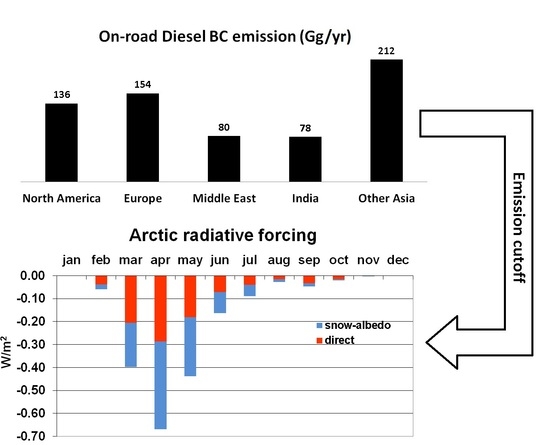
Carbonaceous particles are both primary (BC and OC) and secondary particles (OC), the latter mostly originating from emissions of complex hydrocarbons from vegetation (terpene families) and leading to the formation of the so-called secondary organic aerosols (SOA). Anthropogenic combustion produces primary carbonaceous particles with an organic fraction (OC) or pure elemental carbon (BC). BC particles have a large hydrophobic fraction, with a bulk density of approximately 1.7 g·cm−3 [6] and a size distribution in the accumulation mode with a mean radius close to 0.07–0.1 µm (see, for example, Schwarz et al. [43] and Pueschel and Kinne [44]). Sulfate (SO4) and OC, on the other hand, are highly soluble particles.
The most important difference among these aerosol families, however, is in the optical characteristics of the particles, with SO4 and OC acting as almost purely scattering aerosols in the visible range of the solar spectrum. BC, in contrast, has a significant imaginary part of the refractive index and a single scattering albedo in the visible range close to 0.4–0.5 when an organic material coating of ~50 nm in thickness is considered [43]. These characteristics imply a strong absorbing capacity of BC aerosols, which produces a warming in the vertical layer containing BC particles. If the surface albedo is sufficiently high, the resulting radiative forcing will be positive, due to the BC optical depth, and have a high normalized value per unit optical depth. OC and SO4, in turn, tend to cool the surface both directly, by increasing the atmospheric reflectivity, and indirectly, by acting as cloud condensation nuclei. More cloud droplets, in turn, may increase the equivalent surface-atmosphere albedo. The aerosol-cloud indirect effect, however, is not considered in the present study.
In a remote site (such as the Arctic region), the aerosol concentration is determined by spatial-temporal features of planetary-scale transport and by the efficiency of anthropogenic emissions in the polluted source regions, coupled to local removal processes. Consequently, a meaningful impact study on aerosols located in a remote region requires good knowledge of the anthropogenic emissions in the source regions (1), their potential perturbations related to trends or pollution-control measures (such as a limitation of on-road diesel engines) (2), the efficiency of irreversible loss rates (3) and a proper description of the large-scale transport pathways towards the receptor region (4). The Arctic region is vulnerable to BC transport from Northern Hemisphere mid-latitude source regions; over the Arctic, not only is the radiative efficiency of BC the highest, but its snow-albedo forcing is also potentially important [19].

2.3. BC Emissions

According to WMO [16] (World Meteorological Organization), open biomass burning dominates BC emissions on a global scale (41%), with the largest contribution from the tropics. Total land transportation accounts for 19% of the total and 37% of the anthropogenic fraction; diesel on-road transportation emissions account for 10% of the total and 19% of the anthropogenic fraction. Figure 1 is adapted from Bond et al. [13] and shows the on-road diesel percent fraction of total land transportation BC emissions on a regional basis and on-road diesel and total BC emissions in absolute units. The relative contribution of BC emissions from on-road diesel is close to 50% of the total land transport BC emissions in western industrialized countries. The relative contribution of on-road diesel to total BC emissions ranges from 2% in China to 29% in Europe and 48% in the Middle East. As mentioned above, gridded emissions for the year 2000 are taken from the CCMI database [31,32].
Figure 1. (a) On-road diesel percent fraction of total land transport black carbon (BC) emissions (regional). (b) On-road diesel and total BC emissions (Gg/yr) (regional). Adapted from Bond et al. [13].
Atmosphere 06 00318 g001

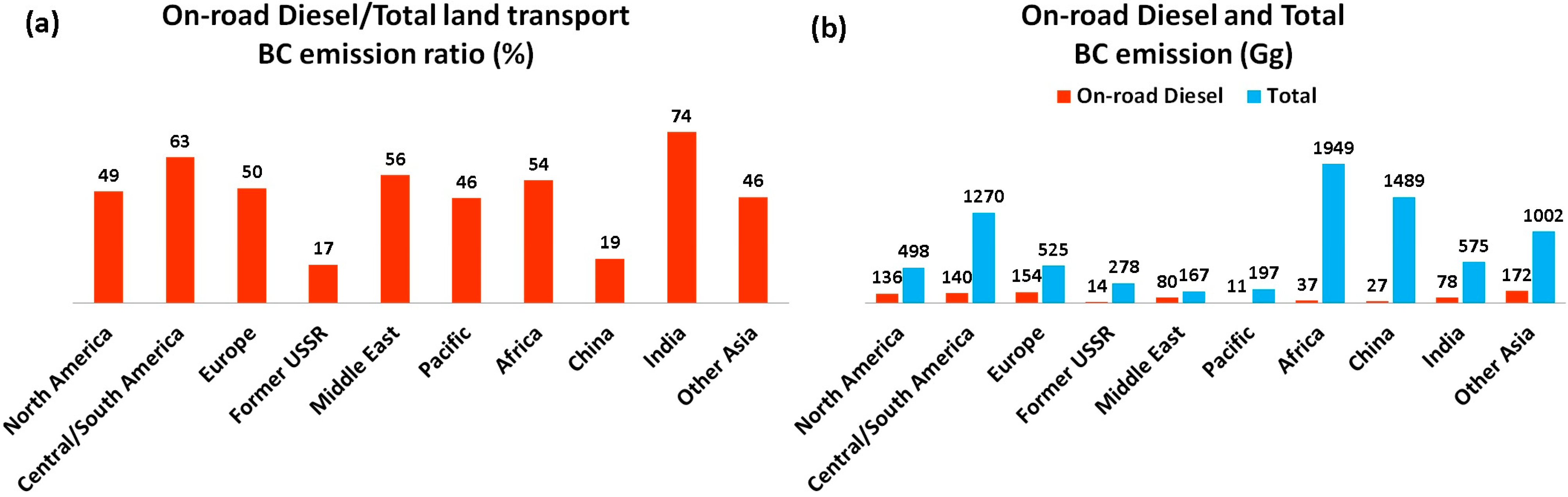
2.4. Numerical Experiment Setup

This study is organized through a baseline experiment (“base”) with anthropogenic fossil fuel emissions of BC, OC and SO2 from the year 2000 and with (climatological) biomass burning sources and a perturbed experiment (“pert”), where on-road diesel emissions of BC particles are removed from the total land transportation sources, using the regional fractions of Figure 1a. These fractions represent a contribution of 27% and 29% of total BC emissions over North America and Europe, respectively, and 14% and 17% over India and East Asia, respectively, excluding China (2%), where BC emissions from on-road diesel are relatively low compared to domestic fire or other non-transportation burning sources. Both “base” and “pert” simulations are run for 6 model years (2000–2005) after a 2-year spin-up (1998–1999); the results for aerosol and gas species are then averaged over 2000–2005 to allow for more robust calculations of anomalies (i.e., “pert”-“base”). The sensitivity approach outlined in this work should be intended as an upper limit of the feasible mitigation, because no displacement of other engine propulsion forms is considered here. In addition to these two main experiments, five additional sensitivity studies were carried out to quantify the model transport of BC from source regions to the Arctic (see the summary in Table 1 and the discussion on BC aircraft emissions).
Table 1. Percent contribution of Northern Hemisphere regional emissions to the Arctic optical thickness of BC (65°N–90°N). Annual average.
Δτ (%)
Europe33
Russia32
Asia27
North America8

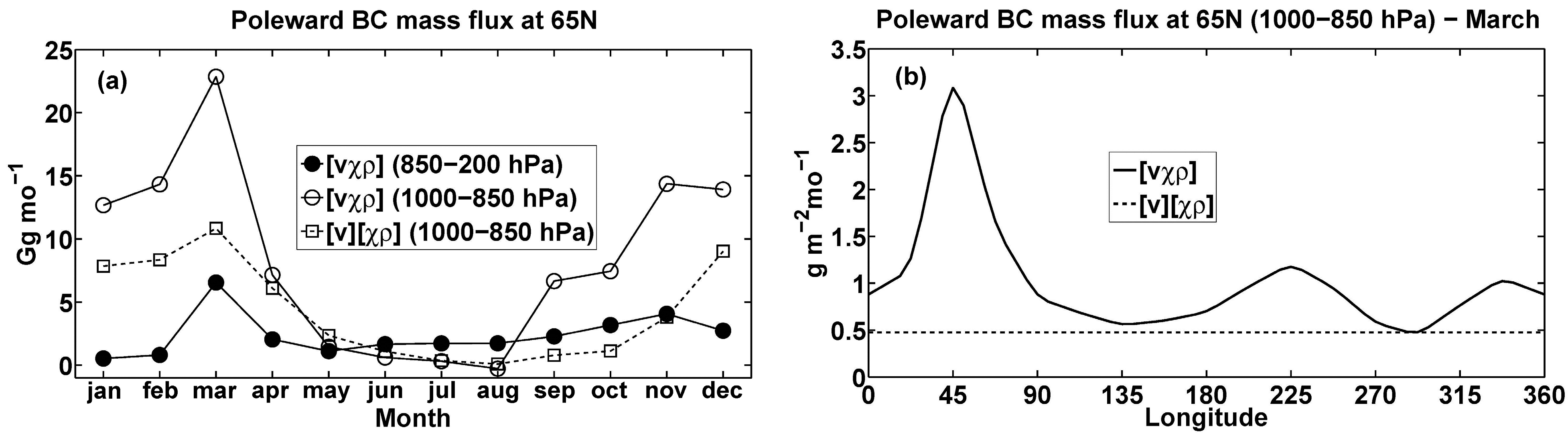
3. Results and Discussion

The model calculated global BC burden is 0.27 Tg C with an average lifetime of 7.2 d; BC global removal is approximately 65% by wet deposition and 35% by dry deposition (77% and 23%, respectively, over the Arctic region, 65°N–90°N), consistent with global budgets reported in Koch and Hansen [18]. Global AeroCom statistics reported in Textor et al. [32] give a mean value of 79% for BC wet deposition among six models, with a 10% standard deviation. Detailed results are discussed in the following subsections, starting from an evaluation of the aerosol results with available observations in the Arctic region. The impact of the removal of on-road diesel emissions is then discussed, both on the calculated BC optical thickness and on the radiation budget.

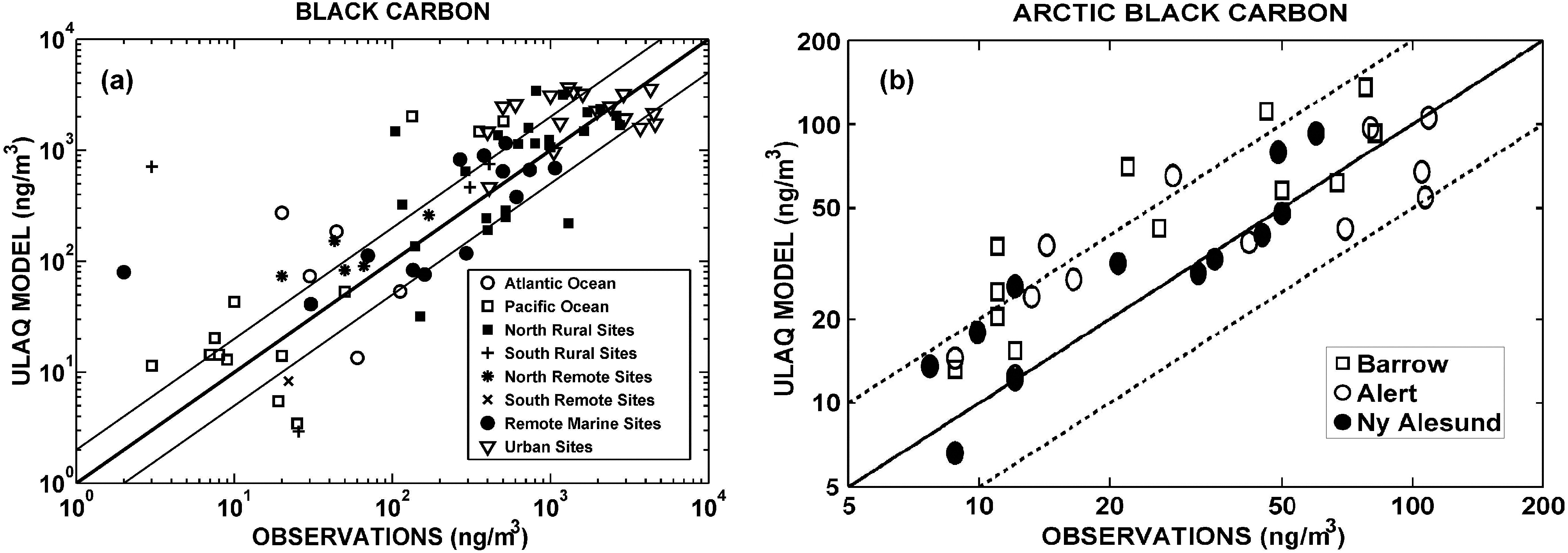
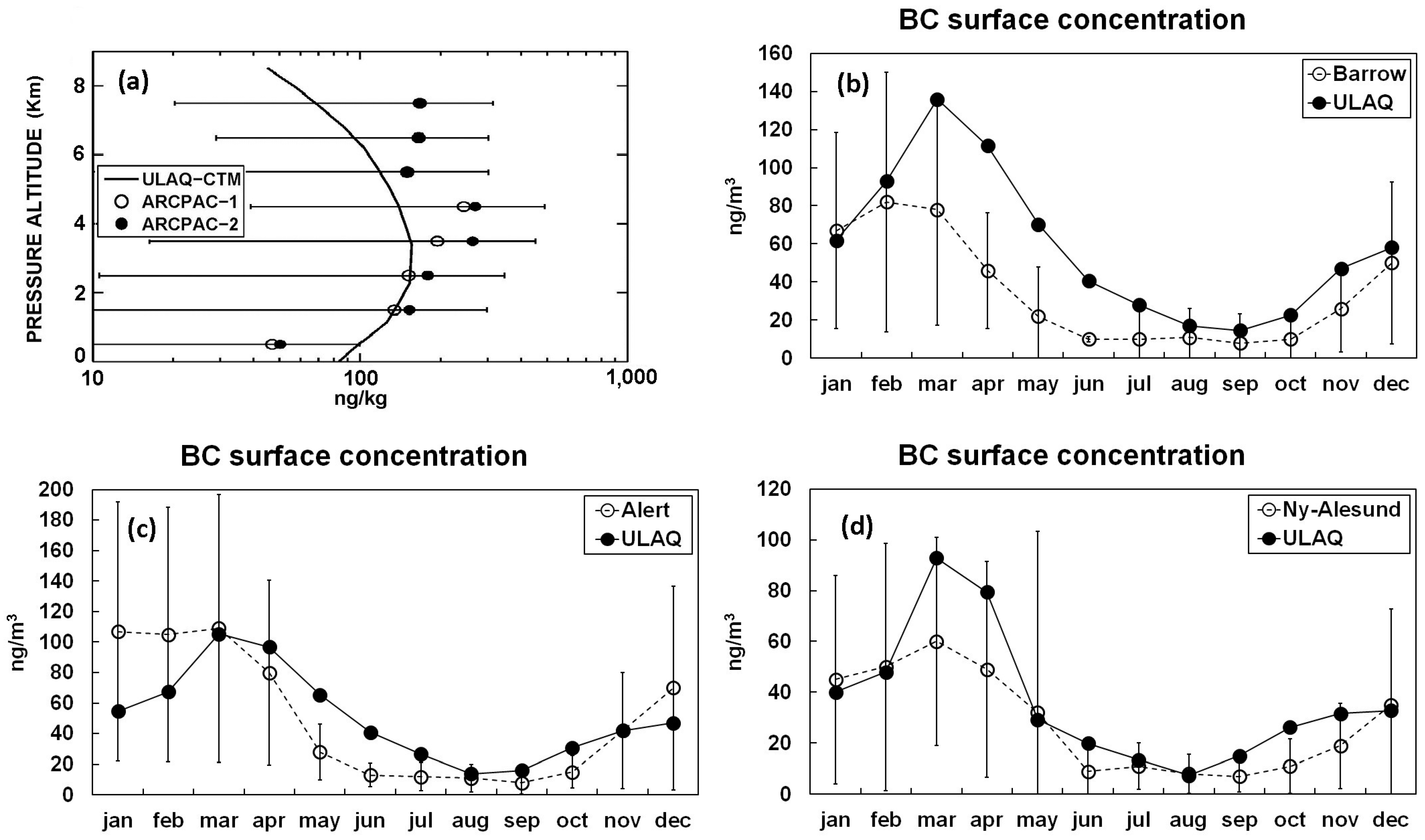
3.1. Evaluation of Model Results with Observations

A comparison of model results for the surface mass concentration of BC with observations on selected worldwide measurement sites is presented in Figure 2a, with the thin lines highlighting a factor of two deviations. The observations used here are those referenced by Liousse et al. [45] and Penner et al. [34]. A similar evaluation of the model results is made for the Arctic region in Figure 2b, using monthly averaged values over three Arctic stations (Barrow, Alert and Ny Alesund). In this case, the observed values are decadal averages reported in Quinn et al. [46] and Sharma et al. [47]. A model overestimation is observed at Barrow during the BC peak concentration time of the year (i.e., springtime) and a systematic positive bias for the summertime minimum values at all stations (see Figure 3).
Figure 3a is an example of the model calculated BC mass mixing ratio vertical profile in the Arctic Pacific region compared to aircraft measurements made during the NOAA ARCPAC campaign during April, 2008 [43]. The model features a maximum in the vertical profile at approximately 3.5 km altitude close to 150 ng/kg, consistent with observations, although the mixing ratio decline above this height is less evident in the observations. The ARCPAC measured increase in BC concentration with altitude is consistent with the aircraft observations of Rosen et al. [48]: they reported that BC in aircraft observations over Barrow increases by a factor of three above the boundary layer. The ULAQ model calculates an increase by a factor 1.8 in the BC mass mixing ratio at 3.5 km altitude with respect to the surface. However, the BC vertical profile predicted in the ULAQ model is in the uncertainty bar of the measurements at all heights and is improved with respect to previous calculations [38], mostly due to a better representation of wet deposition. Recent AeroCom Phase II studies [49], targeted at global BC circulation modelling, clearly state the need for more extensive flight measurement campaigns to properly characterize the long-range BC transport and its atmospheric lifetime.
Figure 2. (a) Scatter plot of calculated versus observed annual mean BC mass concentration values (ng/m3) at selected worldwide locations (see the text and legend). (b) Same as in (a), but for monthly averaged values at three selected Arctic stations (see the text and legend). Thin (or dashed) lines highlight a factor of two deviations.
Atmosphere 06 00318 g002
Figure 3. (a) Vertical profile of the model calculated BC mass mixing ratio (ng/kg) compared to airborne measurements taken during the ARCPAC campaign (April, 2008, Arctic Pacific flights) [43]. (bd) Seasonal cycle of surface mass density (ng/m3) from the model, compared to observations at selected Arctic stations: Barrow (71°N, 156.6°W), Alert (82°N, 62.3°W) and Ny-Alesund (79°N, 12°E), respectively [46,47].
Atmosphere 06 00318 g003
Figure 3b–d compares the modelled BC seasonal cycle over the three Arctic stations in Figure 2b with decadal averages from available observations [46,47]. Filter-based absorption instruments at these Arctic stations include the Particle Soot Absorption Photometer (PSAP) and the Aethalometer. The modelled BC concentration seasonal changes appear to be quite similar to the findings from the ACCMIP model inter-comparison [50] (The Atmospheric Chemistry and Climate Model Intercomparison Project). For the three considered measurement sites (Barrow, Alert and Ny-Alesund), northern Eurasia has been identified as the major source region, especially in winter/spring. The ULAQ model is consistent at all three stations, except for a significant overestimation at Barrow during springtime months and some overestimation of the summer minimum at all stations. As discussed in the report of Quinn et al. [45], the models’ ability to reproduce observed measurements can be heavily impaired by the treatment of BC microphysical properties and removal rates. A general behavior is shown by several models discussed in the report to underestimate winter/spring and to overestimate summer/fall BC concentrations in the Arctic. The ULAQ model overestimation during fall months is in the uncertainty interval of the recorded observations, whereas springtime BC concentrations are overestimated, particularly at Barrow.

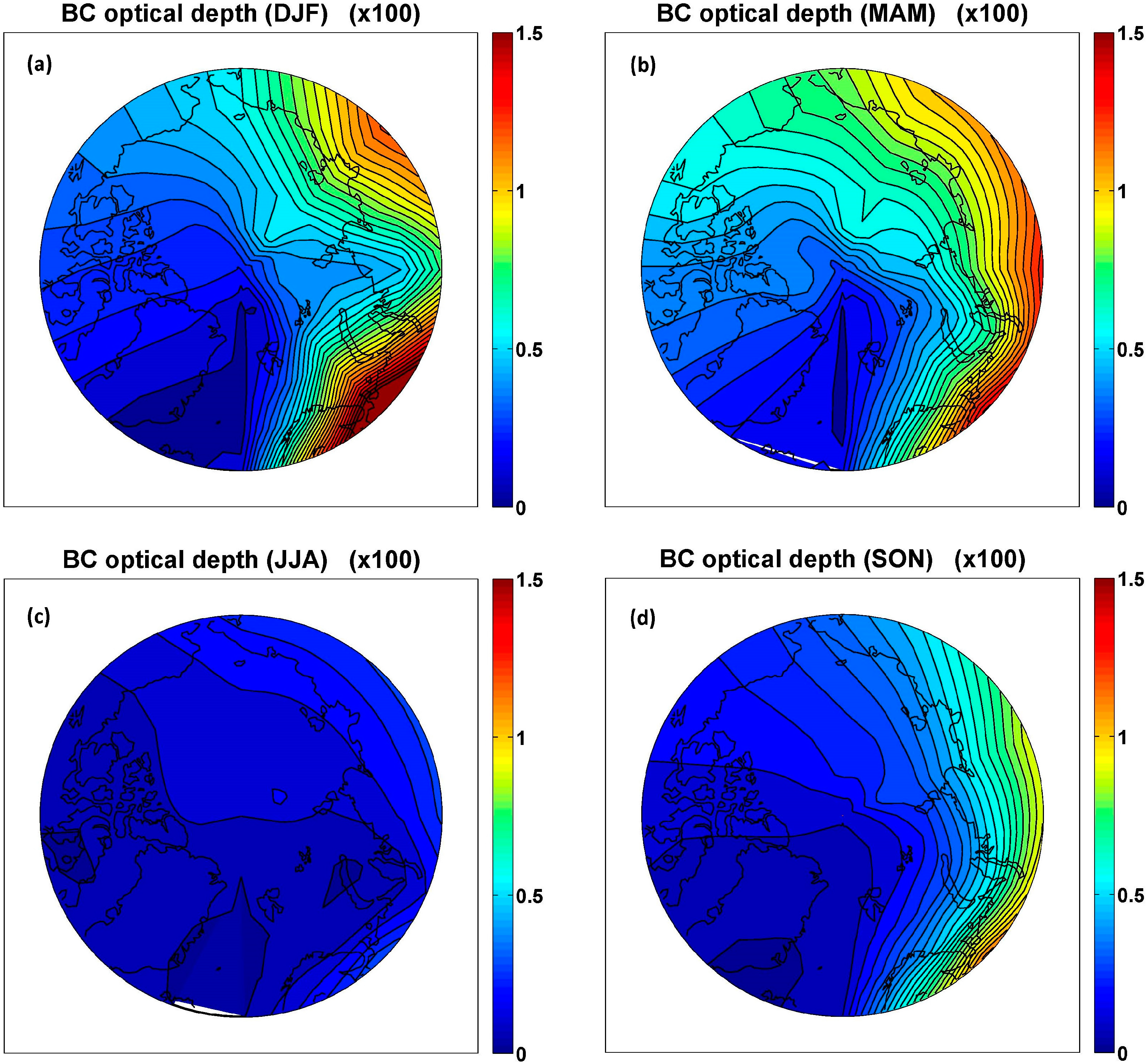
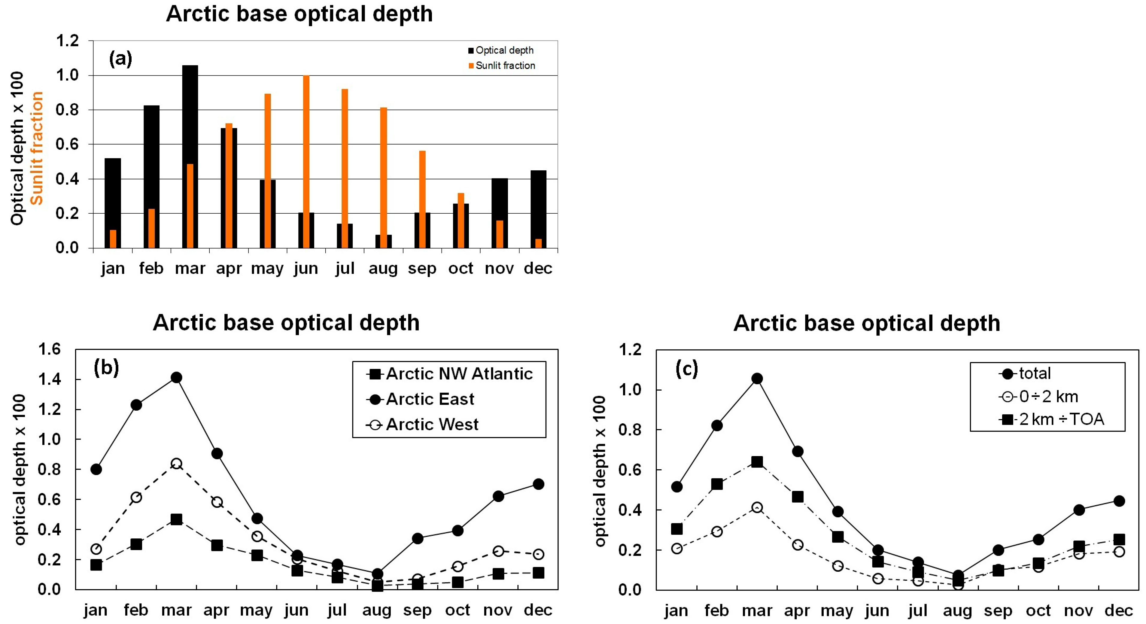
3.2. Discussion of Model Results

Mie scattering properties relevant to the modelled BC size distribution have been calculated through a standard Mie scattering code [41] to provide the wavelength-dependent optical properties needed for a radiation transfer analysis and for calculating the BC optical thickness from the mass density distribution. Several BC aerosol size distribution measurement campaigns provide a quite accurate estimate of the lognormal distribution parameters for transported BC aerosols [43,44]. Accordingly, an effective radius of 0.14 µm has been selected as the input to the Mie code (0.05 µm of which are due to coating thickness) [43,51]. The BC complex refraction index is taken from Bond et al. (2013) [6]. A single scattering albedo of 0.45 is calculated at λ = 0.55 µm, with a refraction index of 1.95-0.79i at the same wavelength. For biomass burning BC, the single scattering albedo is increased to 0.75.
The model-calculated optical thickness of black carbon aerosols and its seasonal evolution in the Arctic region are presented in Figure 4. Consistent with other model calculations [18], the larger values on the eastern Arctic and the shape of the contour lines highlight the important role of the large-scale transport of BC aerosols from Eurasian sources. Table 1 presents a summary on an annual basis of the model calculated continental contributions to Arctic BC.
According to the model, Europe and Russia together (including both industrial sources and biomass burning) provide the major input to the Arctic BC optical thickness. These sources, along with those from Southeast Asia, also provide substantial input to the Western Arctic BC and over the Atlantic, through coupling of the subarctic Westerlies and northward eddy mass fluxes in the atmospheric layers above the surface. The contribution of aircraft emitted BC is negligible in terms of total optical depth (<1%), but larger in the Arctic upper troposphere and lower stratosphere (UTLS): the ULAQ model calculates an aircraft contribution of 4.5% on an annual basis, using the base case emission scenarios adopted from the EC-REACT4C project [52] with an average soot emission index of 0.013 g/kg-fuel at cruise altitudes. Although the UTLS direct effect of BC aircraft emissions is small, their potential climate impact could be significant through indirect formation of “soot-cirrus” particles when ice super-saturation conditions are found, and ice particle formation may occur via heterogeneous freezing [53].
Figure 4. Model calculated BC optical thickness (×100) at λ = 0.55 µm in the Arctic region: (ad) from top left to bottom right, for December-January-February (DJF), March-April-May (MAM), June-July-August (JJA), September-October-November (SON) averages, respectively. The contour line step of optical thickness (×100) is 0.05, starting from 0.15, 0.20, 0.05 and 0.10 in (a–d), respectively, with values of minimum optical depth located on the NW Atlantic.
Atmosphere 06 00318 g004
The pronounced seasonal cycle of Arctic BC optical depth is evident looking at the 65°N–90°N monthly averaged values in Figure 5a,b, where the seasonal cycle per geographical sector is presented. Values are generally between 0.003 and 0.008 throughout the Arctic during winter and spring, except over Greenland and the northwest Atlantic, where it is less (see Figure 4 and Figure 5b), and over the Eastern Arctic during February and March, where values are between 0.012 and 0.014. Optical depth values smaller than 0.003 are predicted during summer and fall seasons when subarctic Westerlies and northward transport due to eddy mass fluxes and mean meridional winds are less pronounced than during winter and spring months. Maximum BC transport is predicted in the model in the late winter and early spring, during Arctic haze transport events, when the greatest transport of pollutants occurs in the boundary layer [54]; a peak of the calculated BC optical thickness is visible during March (0.004) in the lowest 2 km altitude (Figure 5c). The modelled optical thickness during February-March-April is a factor of two higher with respect to the annual average, and the seasonality (i.e., winter-summer difference) is stronger over the eastern Arctic compared to the western Arctic.
Figure 5. (a) Monthly averaged values of model calculated BC optical thickness at λ = 0.55 µm in the Arctic region (65°N–90°N), with the sunlight fractional coverage superimposed. (b) As in (a), but over longitude ranges 60°W–10°E, 10°E–180°E and 180°E–60°W. (c) As in (a), but also for altitude layers 0–2 km and 2 km up to the top of the atmosphere (TOA).
Atmosphere 06 00318 g005
The insights of the model large-scale transport towards the Arctic can be obtained from Figure 6a; in this way, the modelled optical thickness seasonal behavior reported in Figure 5b,c can be better explained, as well as the time series of surface BC mass concentrations in Figure 3b–d. The mean meridional BC mass flux [vχρ] at 65°N (positive northward, i.e., the Arctic influx) is shown for the free troposphere and for the boundary layer (up to 850 hPa). In the latter case, the mean meridional circulation component of the flux [v][χρ] is also presented ([] indicates a zonal average). The dominant role of eddy mass fluxes {[v'(χρ)'] = [vχρ]-[v][χρ]} is evident during the Arctic haze period close to the surface, as reported in the real world (Barrie, 1986). The most favorable conditions for efficient northward transport are found in the model over the Atlantic/European region and in the North American Pacific (Figure 6b), consistent with observations [55]. Hansen and Nazarenko [21] note that these observed features of BC transport towards the Arctic are produced by meteorological blocking conditions during winter-spring months, driving the circulation around the Icelandic low and Siberian high.
Model-calculated changes in the Arctic averaged optical thickness due to the cancellation of on-road diesel sources are shown in Figure 7a (i.e., “pert”-“base” differences) and closely follow the same seasonal cycle of the baseline reference optical depth shown in Figure 5a, with a rather flat relative decrease during the year (16.5% ± 2%) (Figure 7b). This is indirect evidence that the greatest amount of BC loading over the Arctic is transported from NH mid-latitude sources and may therefore be significantly affected by changes in anthropogenic fossil fuel burning, both in terms of decadal trends and the potential regulating measures of these emissions. On a global scale, the BC optical thickness decrease in the sensitivity experiment is calculated to be 10.5% ± 2% (Figure 7c). The decrease in the relative change in BC optical thickness during summer months (8% in July–August versus 13% in April) results primarily from the impact of biomass burning sources in Russia during these months [56]. The contribution of boreal forest fires may actually be highly variable from year to year due to different meteorological conditions. The ULAQ model does not consider this interannual variability, because it uses a climatological inventory dataset for open biomass burning emissions.
Figure 6. (a) Time series of the mean zonal poleward BC mass flux at 65°N latitude (Gg/month), calculated as [vχρ], where [] indicates a zonal average, χ is the BC mass mixing ratio, ρ is the atmospheric mass density and v the meridional wind. The dashed line is for the boundary layer mass flux (1000–850 hPa) due to the mean meridional circulation only {[v][χρ]}. (b) March average of the poleward BC mass flux at 65°N latitude (g·m−2·mo−1) in the boundary layer (1000–850 hPa) as a function of longitude {[vχρ]}. The dashed line is the flux due to the mean meridional wind only; [] indicates a zonal average.
Atmosphere 06 00318 g006
Figure 7. (a) Monthly averaged values of model calculated BC optical thickness changes at λ = 0.55 µm averaged over the Arctic region (65°N–90°N), with changes due to the cancellation of on-road diesel emissions of BC with respect to the base case (“pert”-“base”; pert, perturbed). (b) As in (a), but for percent changes. (c) Monthly-averaged global percent changes.
Atmosphere 06 00318 g007

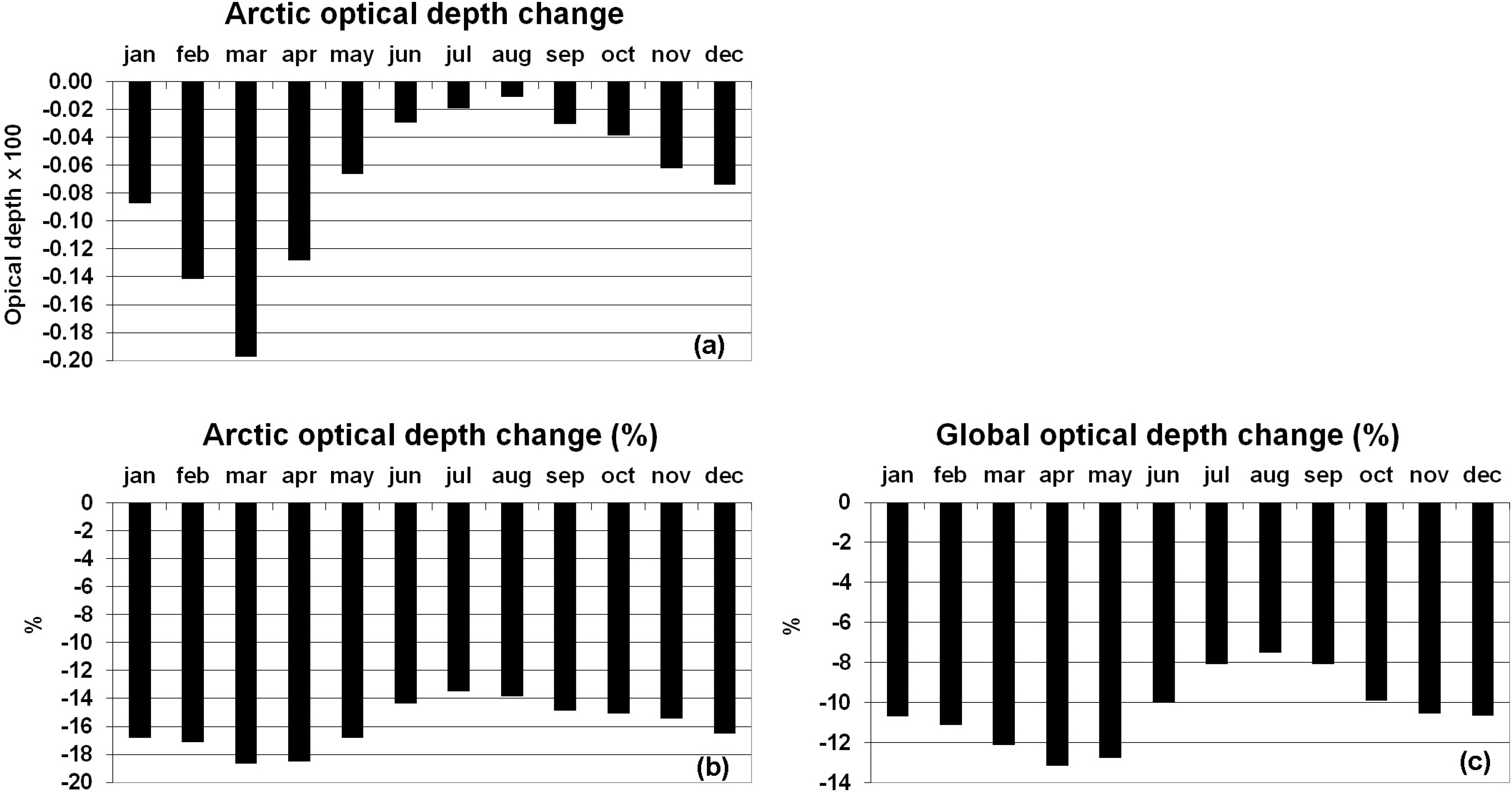
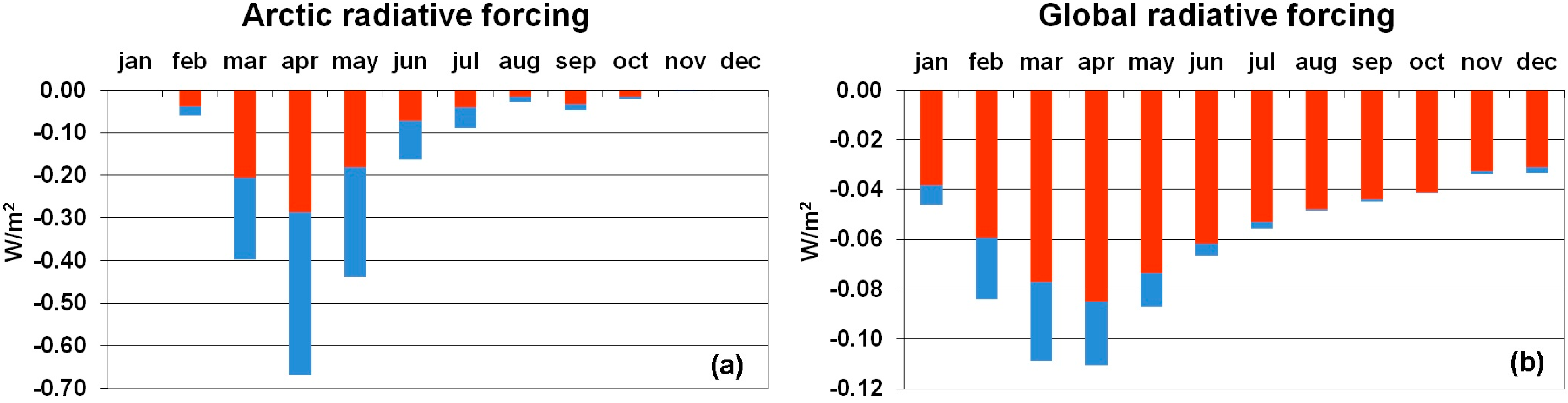
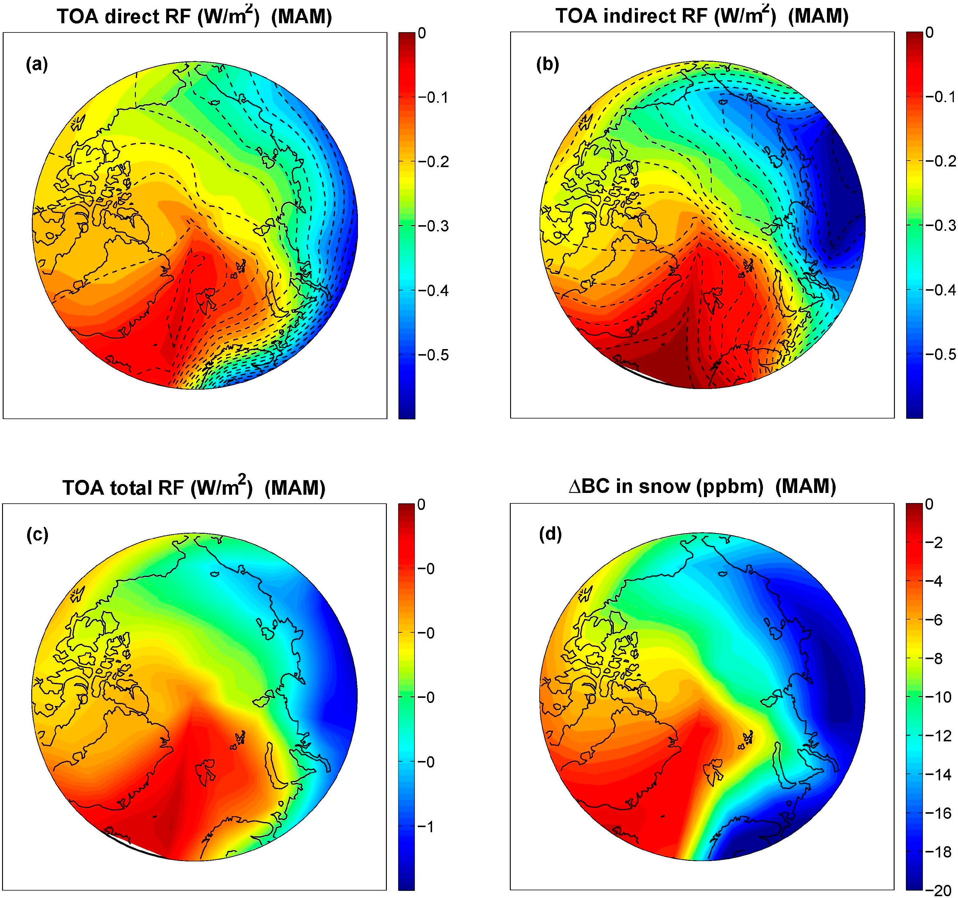
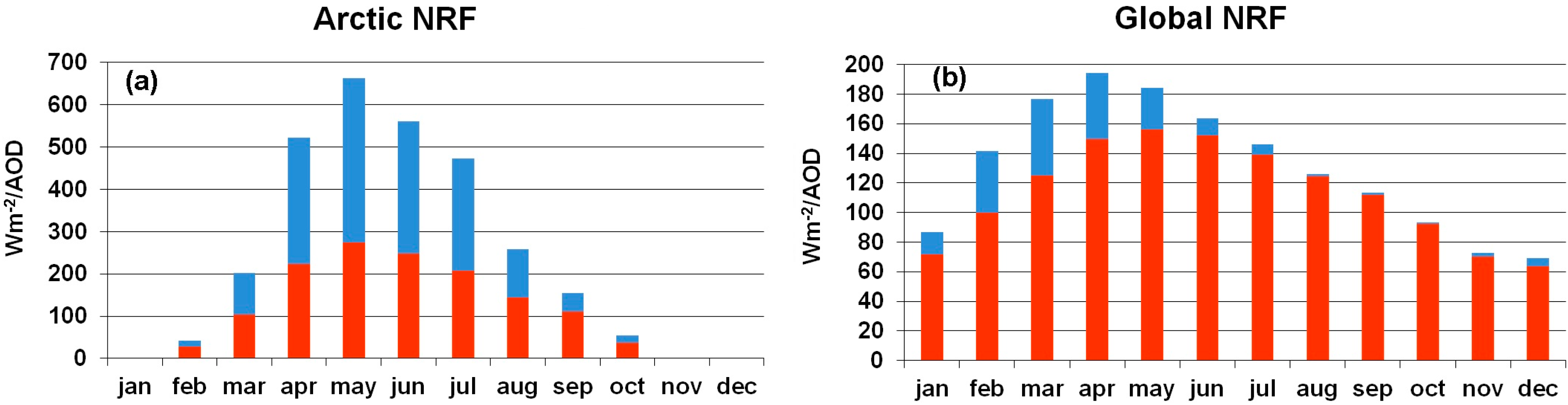
3.3. Radiative Calculations

Except when specified, RF values discussed in this section are calculated in total sky conditions at the tropopause. The Arctic regional radiative forcing associated with the BC perturbation described above is shown in Figure 8a, whereas Figure 8b refers to the globally-averaged RF; here, the direct radiative impact is shown along with the BC snow-albedo forcing. The springtime peak in Arctic BC RF (Figure 8a) is due to coupling of the maximum optical depth change and the incoming solar radiation increase with respect to the winter months (see Figure 5a). As pointed out in Flanner [20], April–May tropospheric BC induces the greatest normalized radiative impact in the Arctic, because high insolation and surface albedo help reach a large specific forcing. According to the model, the average direct RF in the Arctic during March-April-May amounts to −0.22 W∙m−2, to be compared with an annual global average of −0.054 W∙m−2 and an annual Arctic average of −0.074 W∙m−2 (see Table 2). Including the BC snow-albedo forcing, these RF values increase to −0.50, −0.064, −0.16 W∙m−2, respectively.
Figure 8. Monthly averaged values of tropopause radiative forcing (W∙m−2) due to model calculated BC optical depth changes from the cancellation of on-road diesel emissions of BC with respect to the base case (“pert”-“base”). (a,b) Arctic and global averages, respectively. Red/blue bars are for direct and snow-albedo radiative forcings (RFs), respectively.
Atmosphere 06 00318 g008
Table 2. BC optical thickness “pert-base” changes at λ = 0.55 µm, related radiative forcing (W∙m−2) and normalized radiative forcing (NRF) (W/m2/Δτ) averaged over the Arctic region (65°N–90°N) and globally. NRF is computed on a monthly basis, then the yearly average is taken. The fifth column shows the BC mixing ratio “pert-base” changes in Arctic snow due to wet and dry deposition.
Δτ (×100)Direct RF (W∙m−2)Direct NRF (W/m2/Δτ)Snow-Albedo RF (W∙m−2)BC in Arctic Snow (ppbm)Total RF (W∙m−2)Total NRF (W/m2/Δτ)
Arctic annual−0.074−0.074110−0.0866.0 ± 3.6−0.16240
Global annual−0.048−0.054115−0.010−0.064130
Arctic MAM−0.13−0.22200−0.2810.5 ± 5.5−0.50460
Global MAM−0.055−0.079145−0.023−0.10185
A potential overestimate of the calculated spring-summer RF values may be expected when considering the ULAQ model tendency to overestimate surface BC values at some Arctic locations (see, for example, Figure 3b,c). Note also how the seasonal cycle of the global RF (Figure 8b) is similar to the Arctic RF, indicating the significant radiative impact of poleward-transported BC. The BC direct radiative effect in the ULAQ model exhibits a clear dependence on its vertical distribution, with a significantly higher forcing efficiency at altitudes above 5 km (see Table 3), consistent with the findings of Samset et al. [57]. As in our case, they show an efficiency increase with increasing altitude and a decrease when approaching the tropopause.
Table 3. Calculated BC radiative forcing efficiency (W/m2/Δτ) as a function of altitude, for clear sky and total sky conditions (Arctic MAM).
Pressure Layer (hPa)Direct NRF Clear Sky (W/m2/Δτ)Direct NRF Total Sky (W/m2/Δτ)
334–2848799
393–334207220
463–393203215
544–463198210
640–544193203
753–640187184
885–753182171
1000–885176164
Snow/ice albedo changes due to BC deposition are not explicitly calculated in this study. However, the annually averaged BC deposition over Arctic snow/ice resulting from the baseline model simulation implies a BC mass mixing ratio in surface H2O of 36 ± 22 ppbm (see Table 4), with uncertainty related to the geographical dispersion, and this value is consistent with that reported by Hansen and Nazarenko [21] (i.e., 30 ppbm mean value and 4 ppbm over Greenland, where minimum BC deposition is recorded). For this reason, their same albedo perturbation is applied here (i.e., 1.5% on Arctic and 3% on snow-covered northern mid-latitudes), although substantial uncertainty must be admitted, because the actual albedo perturbation is a function of important microphysical factors (in particular, the internal/external mixing of BC and fresh/old snow conditions). The 1.5% relative change in snow/ice albedo over the Arctic region has to be considered a spatially, annually and spectrally averaged value, with a 2.5% change imposed for λ < 0.77 µm, 1.25% for 0.77 µm < λ < 0.86 µm and no change for λ > 0.86 µm (as in Hansen and Nazarenko [21]).
Table 4. Base case optical thickness of BC at λ = 0.55 µm and related radiative forcing (W∙m−2). The fourth column shows the BC mixing ratio in Arctic snow due to wet and dry deposition.
τ (×100)Direct RF (W∙m−2)Snow-Albedo RF (W∙m−2)BC in Arctic Snow (ppbm)Total RF (W∙m−2)
Arctic annual0.450.430.5136 ± 220.94
Global annual0.460.460.0540.51
Arctic MAM0.721.251.5858 ± 312.83
Global MAM0.450.660.130.79
The model calculated deposition fields at each surface grid box are used to scale these albedo perturbation values; the results of these calculations are summarized in Table 4 for total BC and in Table 2 for the BC reduction due to the cancellation of on-road diesel emissions. According to the model, the corresponding BC/snow global-annual climate forcing is +0.054 W∙m−2 for total BC and −0.010 W∙m−2 for the BC reduction, with Arctic annual average values of +0.51 W∙m−2 and −0.09 W∙m−2, respectively. The albedo perturbation estimated in Hansen and Nazarenko [21] yields a climate forcing of +0.3 W∙m−2 in the Northern Hemisphere (i.e., ~+0.15 W∙m−2 globally). In addition, they noted that the efficacy of this indirect soot forcing is ~2, which is twice as effective as CO2 in altering global surface air temperature for a given radiative forcing. It represents for this reason an important driving mechanism for recent trends in sea/ice temperatures over the Arctic region. Their forcing is then a factor three larger with respect to the one calculated here. However, it was subsequently corrected in Hansen et al. [58] and Hansen et al. [59] to +0.05 W∙m−2 (globally) by scaling the BC/snow forcing on gridded deposition fields (as in our case) instead of assuming spatially-annually uniform snow albedo reductions over Arctic sea-ice and Northern Hemisphere snow-covered land, as discussed in Flanner et al. [60].
Figure 9a clearly shows how the springtime polar RF contour lines follow the optical depth change contours and highlight transport streamlines from coupled subarctic Westerlies and northward transport. Available observations show high tropospheric BC concentrations over the Arctic up to 8 km in altitude, with magnitudes comparable to profiles measured over polluted areas at northern mid-latitudes [48], thus demonstrating the role of global atmospheric transport mechanisms. As discussed above, the consequent significant BC deposition over Arctic snow and ice tends to reduce the surface albedo [19], thus indirectly contributing to regional (and global) warming. The direct climate effect of Arctic BC is related to the absorption of solar radiation that is efficiently reflected upwards by the snow/ice covered surface, preventing a significant fraction of the surface reflected solar radiation to reach the top of the atmosphere. The latter is a form of radiative process similar to that of greenhouse gases, but acting on solar shortwave radiation instead of on longwave blackbody planetary radiation.
Figure 9b presents model results for the BC snow-albedo RF due to the removal of on-road diesel emissions (spring months): RF contours closely follow the calculated albedo changes, except for some non-linear effects arising from the superposition of spatial inhomogeneity in surface albedo and the distribution of atmospheric absorbers (namely, BC). The total BC RF (direct + snow-albedo effect) arising from the emission perturbation is presented in Figure 9c by summing the contributions in the previous two panels; this value reaches approximately −1.0 W∙m−2 during spring months over the eastern Arctic region. As discussed above, the snow-albedo BC forcing is calculated on the basis of the perturbation of BC deposition fields (wet + dry). These are shown in Figure 9d and range between approximately 3 and 20 ppbm (i.e., ng-BC/g-H2O) over Iceland and Siberia, respectively. The snow-albedo BC forcing presented in Figure 9b follows the calculated changes in BC deposition, except over the NE Atlantic and northern Scandinavia, where surface albedo (and its absolute changes due to BC deposition) are much smaller than in all other parts of the Arctic region. On average, annually, the ULAQ model calculates 77% and 23% wet and dry contributions, respectively, to BC Arctic deposition with 0.27 Tg/yr of total deposited BC. As a comparison, Breider et al. [56] calculated 89% and 11% wet and dry contributions, respectively, with 0.28 Tg/y of total deposited BC.
Figure 9. (ac) Model calculated tropopause radiative forcing (W∙m−2) defined as in Figure 8, in the Arctic region (March-April-May average) (color scale): direct, snow-albedo and total RF are presented in (a–c), respectively. Superimposed in (a) are the contour lines of the corresponding BC optical depth changes at λ = 0.55 µm (dashed) and defined as in Figure 7, with a contour line step of −2 × 10⁻⁴ starting from −4 × 10⁻⁴ on the NW Atlantic, up to −4 × 10⁻³. Superimposed in (b) are the contour lines of snow/ice surface albedo absolute changes in the visible wavelength range (dashed), with contour line step −5 × 10⁻⁴ starting from −5 × 10⁻⁴ on the NW Atlantic, up to −8 × 10⁻³. Albedo percent changes are obtained as described in the text, as a linear function of the model calculated changes in BC surface deposition on snow (wet + dry) that are presented in (d) in ppbm (i.e., ng-BC/g-H2O).
Atmosphere 06 00318 g009
Figure 10 shows the radiative forcing per unit optical depth both in the Arctic (Figure 10a) and globally (Figure 10b). As discussed above, the BC forcing efficiency in the Arctic region is strongly affected by the underlying surface albedo, substantially higher than its global average due to permanent snow/ice coverage. The normalized radiative forcing (NRF) shown in Figure 10a and summarized in Table 2 follows the seasonality of the available amount of incoming solar radiation and reaches a maximum of approximately 250 in the Arctic during May and June, to be compared with approximately 150 during the same months on a global scale. These values refer only to the direct forcing, for which the definition of NRF is more appropriate. However, because the perturbation in optical thickness also indirectly drives the change in snow/ice albedo, it is possible to include the effects of both direct and snow-albedo RF in the calculation of the normalized forcing. In this case, the ULAQ-model calculated NRF rises up to 650 in the Arctic region during May, and the global value increases to 190 in April (see Figure 10b). On an annual basis, the calculated direct NRF accounts for 110 and 115 over the Arctic and globally, respectively, and increases to 240 and 130, including also the snow-albedo effect. The annual mean NRF reported in the study of Schulz et al. [22] for total atmospheric BC is 153 ± 68 on a global scale (direct forcing only). During springtime months with the highest BC RF (see Figure 10), the NRF accounts for 200 and 145 (Arctic and global MAM averages, respectively), increasing to 460 and 185 when considering the snow-albedo effect, as visible in (a) and (b) of Figure 10, respectively. The seasonal behavior of the calculated BC forcing efficacy is consistent with the findings of Flanner [20].
Figure 10. Monthly averaged values of normalized radiative forcing (NRF = RF/Δτ) (W∙m−2/Δτ), where Δτ is the BC aerosol optical depth (AOD) change at λ = 0.55 µm, defined as in Figure 7. (a,b) Arctic and global average, respectively. Red/blue bars are for direct and snow-albedo NRFs, respectively.
Atmosphere 06 00318 g010

4. Conclusions

The present study makes use of a climate-chemistry model with an interactive aerosol module to explore the sensitivity of the Arctic concentration of black carbon aerosols to land transportation emissions from mid-latitude source regions. In particular, the beneficial effects of removing BC emissions from on-road diesel engines are explored by calculating the changes in BC optical depth poleward of 65°N and the radiative impact. A global average decrease of 10.5% ± 2% is calculated for BC optical depth at λ = 0.55 µm, along with a 16.5% ± 2% value over the Arctic region, taking into account the seasonal variability. The annual average direct radiative forcing corresponding to these changes is found to be −0.054 W∙m−2 and −0.074 W∙m−2, respectively, which are significant RF values compared to those of other climate agents, in particular the Arctic value. These RF values become significantly larger when considering the snow-albedo effect due to BC wet/dry deposition. According to the model, global and Arctic averages of the annual RF raise up to −0.064 W∙m−2 and −0.16 W∙m−2, respectively.
The rapidly changing regional emission of anthropogenic BC has to be considered as a potential source of uncertainty of the above estimates, as well as possible systematic biases in the emission inventories. If projections for land transportation emissions are used as a robust indication of future trends [61], then there is an indication of a reduction of diesel on-road emissions in 2014 compared to 2000 on the order of 30%. However, the diesel on-road contribution to BC emissions is planned to grow again in the future and return to 2000 values by mid-century, following extensive motorization of highly populated countries in East Asia. A potential future assessment based on multi-model predictions could be useful to narrow the intrinsic uncertainty of the present study, which is related to the model ability to transport pollutants from the source regions (i.e., the Northern Hemisphere mid-latitudes) to the receptor region (i.e., the Arctic). In addition, it should be considered that some non-linear effects on the Arctic mitigation discussed in this work could be expected from year-to-year changes in biomass burning emissions, for which an average climatological value is used here.
Model predictions have first been evaluated using surface BC concentrations observed in three Arctic stations and comparing the calculated high-latitude vertical profile of the BC mass mixing ratio to that observed from aircraft measurements over the Arctic Pacific region. The pronounced seasonality of the calculated Arctic optical thickness is found to be consistent with that from other models (e.g., Koch and Hansen [18]), as well as the calculated differences between eastern and western Arctic values and the role of Eurasian sources in determining a large part of BC loading over the Western Arctic and the North Atlantic. The pronounced seasonal cycle of meridional eddy mass fluxes of BC towards the northern high-latitudes is found to be the most important reason for the BC behavior over the Arctic, in particular for the BC maximum calculated in the model (and observed in the real world) during the Arctic haze period, i.e., late winter and beginning of spring.
On an annual basis, the calculated normalized radiative forcing, i.e., RF normalized to the BC optical depth change at λ = 0.55 µm, accounts for 110 and 115 over the Arctic and globally, respectively, and increases to 240 and 130 when considering the snow-albedo effect. During springtime months with the highest BC RF, the NRF accounts for 200 and 145 over the Arctic and globally, respectively; these values increase to 460 and 185 when considering the BC/albedo effect. These values are consistent with the annual mean NRF reported in the study of Schulz et al. [22] for total atmospheric BC, i.e., 153 ± 68 on a global scale for the direct RF alone, from an average of nine aerosol models. The high BC NRF value over the Arctic region makes large-scale atmospheric transport of BC towards the polar region a significant source of climate forcing; the potential mitigation resulting from the cut-off of on-road diesel emissions should then be considered among those feasible measures to temporarily counteract the effects of growing atmospheric concentrations of long-lived greenhouse gases, CO2 in particular.

Acknowledgments

Part of this work has been completed under the EC project, REACT4C, Grant No. ACP8-GA-2009-233772. The authors would like to acknowledge David Lee and Ling Lim of Manchester Metropolitan University for providing aircraft emission scenarios to be used in the model runs. The authors would like to thank the anonymous reviewers for their helpful suggestions, mostly one on the correct treatment of the BC single scattering albedo.

Author Contributions

Giovanni Pitari: overall coordination and responsibility for the climate-chemistry-transport modules. Glauco Di Genova: BC emissions and radiative calculations. Natalia De Luca: evaluation of the model results with observations.

Conflicts of Interest

The authors declare no conflict of interest.

References

  1. Uherek, E.; Halenka, T.; Borken-Kleefeld, J.; Balkanski, Y.; Berntsen, T.; Borrego, C.; Gauss, M.; Hoor, P.; Juda-Rezler, K.; Lelieveld, J.; et al. Transport impacts on atmosphere and climate: Land transport. Atmos. Env. 2010, 44, 4772–4816. [Google Scholar] [CrossRef]
  2. Shine, K.; Forster, P.M. The effect of human activity on radiative forcing of climate change: A review of recent developments. Glob. Planet. Chang. 1999, 20, 205–225. [Google Scholar] [CrossRef]
  3. Intergovernmental Panel for Climate Change (IPCC). Climate change 2013. In The Physical Science Basis; Stocker, T.F., Qin, D., Plattner, G.-K., Tignor, M.M.B., Allen, S.K., Boschung, J., Nauels, A., Xia, Y., Bex, V., Midgley, P.M., Eds.; Cambridge University Press: Cambridge, UK, 2013; Chapter 7. [Google Scholar]
  4. Fuller, K.A.; Malm, W.C.; Kreidenweis, S.M. Effects of mixing on extinction by carbonaceous particles. J. Geophys. Res. 1999, 104, 15941–15954. [Google Scholar] [CrossRef]
  5. Saleh, R.; Robinson, E.S.; Tkacik, D.S.; Ahern, A.T.; Liu, S.; Aiken, A.C.; Sullivan, R.C.; Presto, A.A.; Dubey, M.K.; Yokelson, R.J.; et al. Brownness of organics in aerosols from biomass burning linked to their black carbon content. Nat. Geosci. 2014, 7, 647–650. [Google Scholar] [CrossRef]
  6. Bond, T.C.; Doherty, S.J.; Fahey, D.W.; Forster, P.M.; Berntsen, T.; DeAngelo, B.J.; Flanner, M.G.; Ghan, S.; Kärcher, B.; Koch, D.; et al. Bounding the role of black carbon in the climate system: A scientific assessment. J. Geophys. Res. 2013, 118, 5380–5552. [Google Scholar]
  7. Cohen, J.B.; Wang, C. Estimating global black carbon emissions using a top-down Kalman filter approach. J. Geophys. Res. 2013. [Google Scholar] [CrossRef]
  8. Brandt, E.B.; Kovacic, M.B.; Lee, G.B.; Gibson, A.M.; Acciani, T.H.; Thomas, H.; Le Cras, T.D.; Ryan, P.H.; Budelsky, A.L.; Hershey, G.K.K. Diesel exhaust particle induction of IL-17A contributes to severe asthma. J. Allergy Clin. Immunol. 2013, 132, 1194–1201. [Google Scholar] [CrossRef] [PubMed]
  9. Suglia, S.F.; Gryparis, A.; Wright, R.O.; Schwartz, J.; Wright, R.J. Association of black carbon with cognition among children in a prospective birth cohort study. Am. J. Epidemiol. 2008, 167, 280–286. [Google Scholar] [CrossRef] [PubMed]
  10. McCracken, J.; Baccarelli, A.; Hoxha, M.; Dioni, L.; Melly, S.; Coull, B.; Suh, H.; Vokonas, P.; Schwartz, J. Annual ambient black carbon associated with shorter telomeres in elderly men: Veterans Affairs Normative Aging Study. Environ. Health Perspect. 2010, 118, 1564–1570. [Google Scholar] [CrossRef] [PubMed]
  11. Riddle, S.G.; Robert, M.; Jakober, C.A.; Hannigan, M.P.; Kleeman, M.J. Size-Resolved source apportionment of airborne particle mass in a roadside environment. Environ. Sci. Technol. 2008, 42, 6580–6586. [Google Scholar] [CrossRef] [PubMed]
  12. Twigg, M.W. Progress and future challenges in controlling automotive exhaust gas emissions. Appl. Catal. B Environ. 2007, 70, 2–15. [Google Scholar] [CrossRef]
  13. Bond, T.C.; Streets, D.G.; Yarber, K.F.; Nelson, S.M.; Woo, J.-H.; Klimont, Z. A technology-based global inventory of black and organic carbon emissions from combustion. J. Geophys. Res. 2004, 109, D14203. [Google Scholar] [CrossRef]
  14. Environmental Protection Agency (EPA). Report to Congress on Black Carbon; EPA-450/R-12–001; Department of the Interior, Environment, and Related Agencies: Research Triangle Park, NC, USA, 2012. [Google Scholar]
  15. Kopp, R.E.; Mauzeralla, D.L. Assessing the climatic benefits of black carbon mitigation. PNAS 2010, 107, 11703–11708. [Google Scholar] [CrossRef] [PubMed]
  16. World Meteorological Organization (WMO). Integrated Assessment of Black Carbon and Tropospheric Ozone; WMO: Geneva, Switzerland, 2011. [Google Scholar]
  17. Pitari, G.; Di Carlo, P.; Coppari, E.; de Luca, N.; Di Genova, G.; Iarlori, M.; Pietropaolo, E.; Rizi, V.; Tuccella, P. Aerosol measurements in central Italy: Impact of local sources and large scale transport resolved by LIDAR. J. Atmos. Solar-Terr. Phys. 2013, 92, 116–123. [Google Scholar] [CrossRef]
  18. Koch, D.; Hansen, J. Distant origins of Arctic black carbon: A Goddard Institute for Space Studies Model E experiment. J. Geophys. Res. 2005, 110, D04204. [Google Scholar] [CrossRef]
  19. Jiao, C.; Flanner, M.G.; Balkanski, Y.; Bauer, S.E.; Bellouin, N.; Berntsen, T.K.; Bian, H.; Carslaw, K.S.; Chin, M.; De Luca, N.; et al. An AeroCom assessment of black carbon in Arctic snow and sea ice. Amos. Chem. Phys. 2014, 14, 2399–2417. [Google Scholar]
  20. Flanner, M.G. Arctic climate sensitivity to local black carbon. J. Geophys. Res. 2013, 118, 1840–1851. [Google Scholar]
  21. Hansen, J.; Nazarenko, L. Soot climate forcing via snow and ice albedos. PNAS 2004, 101, 423–428. [Google Scholar] [CrossRef] [PubMed]
  22. Schulz, M.C.; Textor, S.; Kinne, Y.; Balkanski, S.; Bauer, T.; Berntsen, T.; Berglen, O.; Boucher, F.; Dentener, S.; Guibert, I.S.A.; et al. Radiative forcing by aerosols as derived from the AeroCom present-day and pre-industrial simulations. Atmos. Chem. Phys. 2006, 6, 5225–5246. [Google Scholar] [CrossRef]
  23. Pitari, G.; Mancini, E.; Rizi, V.; Shindell, D.T. Impact of future climate and emission changes on stratospheric aerosols and ozone. J. Atmos. Sci. 2002, 59, 414–440. [Google Scholar] [CrossRef]
  24. Eyring, V.; Butchart, N.; Waugh, D.W.; Akiyoshi, H.; Austin, J.; Bekki, S.; Bodeker, G.E.; Boville, B.A.; Brühl, C.; Chipperfield, M.P.; et al. Assessment of temperature, trace species, and ozone in chemistry-climate model simulation of the recent past. J. Geophys. Res. 2006, 111, D22308. [Google Scholar] [CrossRef]
  25. Morgenstern, O.; Giorgetta, M.A.; Shibata, K.; Eyring, V.; Waugh, D.; Shepherd, T.G.; Akiyoshi, H.; Austin, J.; Baumgärtner, A.; Bekki, S.; et al. A review of CCMVal-2 models and simulations. J. Geophys. Res. 2010. [Google Scholar] [CrossRef]
  26. Kärcher, B.; Lohmann, U. A parameterization of cirrus cloud formation: Homogeneous freezing of supercooled aerosols. J. Geophys. Res. 2002. [Google Scholar] [CrossRef]
  27. Kärcher, B.; Lohmann, U. A parameterization of cirrus cloud formation: Homogeneous freezing including effects of aerosol size. J. Geophys. Res. 2002. [Google Scholar] [CrossRef]
  28. Pitari, G.; Aquila, V.; Kravitz, B.; Robock, A.; Watanabe, S.; Cionni, I.; de Luca, N.; Di Genova, G.; Mancini, E.; Tilmes, S. Stratospheric ozone response to sulfate geoengineering: Results from the Geoengineering Model Intercomparison Project (GeoMIP). J. Geophys. Res. 2014, 119, 2629–2653. [Google Scholar]
  29. Penner, J.E. Carbonaceous aerosols influencing atmospheric radiation: Black carbon. In Aerosol Forcing of Climate; Charlson, R.J., Heintzenberg, J., Eds.; Wiley: Chichester, UK, 1995; pp. 91–108. [Google Scholar]
  30. Koch, D.; Schulz, M.; Kinne, S.; McNaughton, C.; Spackman, J.R.; Bond, T.C.; Balkanski, Y.; Bauer, S.; Berntsen, T.; Boucher, O.; et al. Evaluation of black carbon estimations in Global Aerosol Models. Atmos. Chem. Phys. 2009, 9, 9001–9026. [Google Scholar] [CrossRef]
  31. Lamarque, J.F.; Kyle, G.P.; Meinshausen, M.; Riahi, K.; Smith, S.J.; van Vuuren, D.P.; Conley, A.J.; Vitt, F. Global and regional evolution of short-lived radiatively-active gases and aerosols in the representative concentration pathways. Clim. Chang. 2011, 109, 191–212. [Google Scholar] [CrossRef]
  32. Textor, C.; Schulz, M.; Guibert, S.; Kinne, S.; Balkanski, Y.; Bauer, S.; Berntsen, T.; Berglen, T.; Boucher, O.; Chin, M.; et al. Analysis and quantification of the diversities of aerosol life cycles within AEROCOM. Atmos. Chem. Phys. 2006, 6, 1777–1813. [Google Scholar] [CrossRef]
  33. Kinne, S.; Schulz, M.; Textor, C.; Guibert, S.; Balkanski, Y.; Bauer, S.E.; Berntsen, T.; Berglen, T.; Boucher, O.; Chin, M.; et al. An AeroCom initial assessment—Optical properties in aerosol component modules of global models. Atmos. Chem. Phys. 2006, 6, 1815–1834. [Google Scholar] [CrossRef]
  34. Penner, J.; Hegg, D.; Andreae, M.; Leaitch, D.; Pitari, G.; Annegarn, H.; Murphy, D.; Nganga, J.; Barrie, L.; Feichter, H. Chapter 5: Aerosols and indirect cloud effects. In Climate Change 2001—IPCC Third Assessment Report; Houghton, J., Ding, Y., Griggs, D.J., Noguer, M., van der Linden, P.J., Dai, X., Maskell, K., Johnson, C.A., Eds.; Cambridge University Press: Cambridge, UK, 2001; pp. 289–348. [Google Scholar]
  35. Penner, J.E.; Zhang, S.Y.; Chin, M.; Chuang, C.C.; Feichter, J.; Feng, Y.; Geogdzhayev, I.V.; Ginoux, P.; Herzog, M.; Higurashi, A.; et al. A comparison of model- and satellite-derived optical depth and reflectivity. J. Atmos. Sci. 2001, 59, 441–460. [Google Scholar] [CrossRef]
  36. Kinne, S.; Lohmann, U.; Feichter, J.; Schulz, M.; Timmreck, C.; Ghan, S.; Easter, R.; Chin, M.; Ginoux, P.; Takemura, T.; et al. Monthly averages of aerosol properties: A global comparison among models, satellite data and AERONET ground data. J. Geophys. Res. 2003. [Google Scholar] [CrossRef]
  37. Textor, C.; Schulz, M.; Guibert, S.; Kinne, S.; Balkanski, Y.; Bauer, S.; Berntsen, T.; Berglen, T.; Boucher, O.; Chin, M.; et al. The effect of harmonized emissions on aerosol properties in global models—An AeroCom experiment. Atmos. Chem. Phys. 2007, 7, 4489–4501. [Google Scholar] [CrossRef]
  38. Koch, D.; Schulz, M.; Kinne, S.; McNaughton, C.; Spackman, J.R.; Balkanski, Y.; Bauer, S.; Berntsen, T.; Bond, T.C.; Boucher, O.; et al. Corrigendum to “Evaluation of Black Carbon Estimations in Global Aerosol Models”. published in Atmos. Chem. Phys., 9, 9001–9026, 2009. Atmos. Chem. Phys. 2010, 10, 79–81. [Google Scholar] [CrossRef]
  39. Randles, C.A.; Kinne, S.; Myhre, G.; Schulz, M.; Stier, P.; Fischer, J.; Doppler, L.; Highwood, E.; Ryder, C.; Harris, B.; et al. Intercomparison of shortwave radiative transfer schemes in global aerosol modeling: Results from the AeroCom Radiative Transfer Experiment. Atmos. Chem. Phys. 2013, 13, 2347–2379. [Google Scholar] [CrossRef] [Green Version]
  40. Chou, M.D.; Suarez, M.J. A Solar Radiation Parameterization for Atmospheric Studies; NASA Tech. Rep. TM-1999–104606; NASA Goddard Space Flight Cent.: Greenbelt, MD, USA, 1999. [Google Scholar]
  41. Mishchenko, M.I.; Travis, L.D.; Lacis, A.A. Scattering, Absorption, and Emission of Light by Small Particles; Cambridge University Press: Cambridge, UK, 2002. [Google Scholar]
  42. Chipperfield, M.P.; Liang, Q.; Strahan, S.E.; Morgenstern, O.; Dhomse, S.S.; Abraham, N.L.; Archibald, A.T.; Bekki, S.; Braesicke, P.; Di Genova, G.; et al. Multi-model estimates of atmospheric lifetimes of long-lived ozone-depleting substances: Present and future. J. Geophys. Res. 2014, 119, 2555–2573. [Google Scholar]
  43. Schwarz, J.P.; Spackman, J.R.; Gao, R.S.; Watts, L.A.; Stier, P.; Schulz, M.; Davis, S.M.; Wofsy, S.C.; Fahey, D.W. Global-scale black carbon profiles observed in the remote atmosphere and compared to models. Geophys. Res. Lett. 2010. [Google Scholar] [CrossRef]
  44. Pueschel, R.F.; Kinne, S.A. Physical and radiative rroperties of Arctic atmospheric aerosols. Sci. Tot. Env. 1995, 160/161, 811–824. [Google Scholar] [CrossRef]
  45. Liousse, C.; Penner, J.E.; Chuang, C.; Walton, J.J.; Eddleman, H.; Cachier, H. A global three-dimensional model study of carbonaceous aerosols. J. Geophys. Res. 1996, 101, 19411–19432. [Google Scholar] [CrossRef]
  46. Quinn, P.K.; Stohl, A.; Arneth, A.; Berntsen, T.; Burkhart, J.F.; Christensen, J.; Flanner, M.; Kupiainen, K.; Lihavainen, H.; Shepherd, M.; et al. The Impact of Black Carbon on Arctic Climate; Arctic Monitoring and Assessment Programme (AMAP): Oslo, Norway, 2011. [Google Scholar]
  47. Sharma, S.; Ogren, J.A.; Jefferson, A.; Eleftheriadis, K.; Chan, E.; Quinn, P.K.; Burkhart, J.F. Black Carbon in the Arctic, Arctic Report Card 2013. Available online: http://www.arctic.noaa.gov/reportcard/ (accessed on 12 October 2014).
  48. Rosen, H.; Hansen, A.D.A.; Novakov, T. Role of graphitic carbon particles in radiative transfer in the Arctic haze. Sci. Total Environ. 1984, 36, 103–110. [Google Scholar] [CrossRef]
  49. Samset, B.H.; Myhre, G.; Herber, A.; Kondo, Y.; Li, S.-M.; Moteki, N.; Koike, M.; Oshima, N.; Schwarz, J.P.; Balkanski, Y.; et al. Modelled black carbon radiative forcing and atmospheric lifetime in AeroCom Phase II constrained by aircraft observations. Atmos. Chem. Phys. 2014, 14, 12465–12477. [Google Scholar] [CrossRef]
  50. Lee, Y.H.; Lamarque, J.-F.; Flanner, M.G.; Jiao, C.; Shindell, D.T.; Berntsen, T.; Bisiaux, M.M.; Cao, J.; Collins, W.J.; Curran, M.; et al. Evaluation of preindustrial to present-day black carbon and its albedo forcing from Atmospheric Chemistry and Climate Model Intercomparison Project (ACCMIP). Atmos. Chem. Phys. 2013, 13, 2607–2634. [Google Scholar] [CrossRef]
  51. Cross, E.S.; Onasch, T.B.; Ahern, A.; Wrobel, W.; Slowik, J.G.; Olfert, J.; Lack, D.A.; Massoli, P.; Cappa, C.D.; Schwarz, J.P.; et al. Soot particle studies—instrument inter-comparison—project overview. Aerosol Sci. Technol. 2010, 44, 592–611. [Google Scholar] [CrossRef]
  52. Søvde, O.A.; Skowron, A.; Iachetti, D.; Lim, L.; Owen, B.; Hodnebrog, Ø.; Di Genova, G.; Pitari, G.; Lee, D.S.; Myhre, G.; et al. Aircraft emission mitigation by changing route altitude: A multi-model estimate of aircraft NOx emission impact on O3 photochemistry. Atmos. Env. 2014. [Google Scholar] [CrossRef]
  53. Hendricks, J.; Kärcher, B.; Lohmann, U.; Ponater, M. Do aircraft black carbon emissions affect cirrus clouds on the global scale? Geophys. Res. Lett. 2005, 32, L12814. [Google Scholar] [CrossRef]
  54. Barrie, L.A. Arctic air pollution: An overview of current knowledge. Atmos. Environ. 1986, 20, 643–663. [Google Scholar] [CrossRef]
  55. Iversen, T.; Joranger, E. Arctic air pollution and large scale atmospheric flows. Atmos. Environ. 1985, 19, 2099–2108. [Google Scholar] [CrossRef]
  56. Breider, T.J.; Mickley, L.J.; Jacob, D.J.; Wang, Q.; Fisher, J.A.; Chang, R.Y.-W.; Alexander, B. Annual distributions and sources of Arctic aerosol components, aerosol optical depth, and aerosol absorption. J. Geophys. Res. 2014, 119, 4107–4124. [Google Scholar]
  57. Samset, B.H.; Myhre, G.; Schulz, M.; Balkanski, Y.; Bauer, S.; Berntsen, T.K.; Bian, H.; Bellouin, N.; Diehl, T.; Easter, R.C.; et al. Black carbon vertical profiles strongly affect its radiative forcing uncertainty. Atmos. Chem. Phys. 2013, 13, 2423–2434. [Google Scholar] [CrossRef]
  58. Hansen, J.; Sato, M.; Ruedy, R.; Nazarenko, L.; Lacis, A.; Schmidt, G.A.; Russell, G.; Aleinov, I.; Bauer, M.; Bauer, S.; et al. Efficacy of climate forcings. J. Geophys. Res. 2005, 110, D18104. [Google Scholar] [CrossRef]
  59. Hansen, J.; Sato, M.; Ruedy, R.; Kharecha, P.; Lacis, A.; Miller, R.L.; Nazarenko, L.; Lo, K.; Schmidt, G.A.; Russell, G.; et al. Climate simulations for 1880–2003 with GISS ModelE. Clim. Dyn. 2007, 29, 661–696. [Google Scholar] [CrossRef]
  60. Flanner, M.G.; Zender, C.S.; Randerson, J.T.; Rasch, P.J. Present-day climate forcing and response from black carbon in snow. J. Geophys. Res. 2007, 112, D11202. [Google Scholar] [CrossRef]
  61. Walsh, M.P. On and off road policy strategies. In Proceedings of the ICCT International Workshop on Black Carbon, London, UK, 5 January 2009.

