Neural Fuzzy Inference System-Based Weather Prediction Model and Its Precipitation Predicting Experiment

Abstract

We propose a weather prediction model in this article based on neural network and fuzzy inference system (NFIS-WPM), and then apply it to predict daily fuzzy precipitation given meteorological premises for testing. The model consists of two parts: the first part is the “fuzzy rule-based neural network”, which simulates sequential relations among fuzzy sets using artificial neural network; and the second part is the “neural fuzzy inference system”, which is based on the first part, but could learn new fuzzy rules from the previous ones according to the algorithm we proposed. NFIS-WPM (High Pro) and NFIS-WPM (Ave) are improved versions of this model. It is well known that the need for accurate weather prediction is apparent when considering the benefits. However, the excessive pursuit of accuracy in weather prediction makes some of the “accurate” prediction results meaningless and the numerical prediction model is often complex and time-consuming. By adapting this novel model to a precipitation prediction problem, we make the predicted outcomes of precipitation more accurate and the prediction methods simpler than by using the complex numerical forecasting model that would occupy large computation resources, be time-consuming and which has a low predictive accuracy rate. Accordingly, we achieve more accurate predictive precipitation results than by using traditional artificial neural networks that have low predictive accuracy.

1. Introduction

Fuzzy logic [1,2,3,4] and artificial neural networks (ANNs) [5,6,7,8] are important in the intelligent control of complex systems. A combination of them is widely used in solving classification, pattern recognition problems, and so on.

Previous techniques have already combined neural networks with fuzzy logic, and these techniques can be broadly classified into three categories. The first is called the fuzzy neural networks (FNN) [9,10,11,12], which embeds fuzzy logic into a neural network. The second category is the neural-fuzzy system [13,14], whose activation function of the neural network is a fuzzy operator. The third category is the fuzzy-neural hybrid systems [15,16], where the fuzzy logic engine and the neural network perform separately to produce a result. The purpose of the first and second category is to increase the efficiency of the neural network, while the third category is for controlling problems.

Over the last decade, a great deal of attention has been devoted to the use of ANNs’ weather forecasting [17,18,19,20,21,22] since we can predict weather conditions without knowing the complex physical process of atmosphere. Although this method is much simpler than the numerical forecasting method, scientists find that the exact inputs of a neural network for weather forecasting leads to the non-accuracy of the prediction outputs. Besides, a fact that we cannot omit is that the predictive accuracy rate of precipitation is not good enough, even by using complex and time-consuming numerical forecasting methods. In view of this, we consider the use of fuzzy variables such as the levels of meteorological variables as a point forecast for load and hope to get better predictive results.

Traditionally, ANNs use crisp weather variable as its inputs to predict crisp weather conditions, and in this paper, we use fuzzy weather variables as its inputs and predict the fuzzy weather condition instead. Our neural fuzzy inference system-based weather prediction model (NFIS-WPM) could infer a new reasonable fuzzy variable output according to the fuzzy variable inputs by using the algorithm we proposed in this paper and then we use this approach in weather forecasting.

In addition, NFIS-WPM is based on another technique that combines ANNs and fuzzy logic. This technique is different from the previous three techniques since it embeds neural network into fuzzy logic engine with fuzzy input and fuzzy output values. In other words, the first approach and the new approach operate in opposite ways. Besides, this new technique is specifically designed for fuzzy inference problems and the others have different goals.

In this paper, we begin by introducing the basic concepts of fuzzy logic, ANNs and weather forecast in the Preliminaries Section. Then, we propose a weather prediction model based on neural network and fuzzy inference system named “Neural fuzzy inference system-based weather prediction model (NFIS-WPM)”. We also use 3-year summer half meteorological observation data in Taiyuan (a city in Shanxi, China) to test the NFIS-WPM and show how NFIS-WPM operates. Experimental results over a relatively long period of time confirm that the NFIS-WPM can be effectively used in precipitation forecast, and show increased skills compared with the traditional ANNs. Thus, we can expect that NFIS-WPM would have the similar high capability with predictions in other meteorological elements and locations.

2. Preliminaries

2.1. Fuzzy Logic

Fuzzy logic is applied to deal with the notion of biased correctness, in which the value may be between absolutely true and false. Besides, these degrees may be administrated by membership function that is a mapping from a set U to the interval [0,1] when we use linguistic variables [23,24].

A unique membership function [25,26] denoted by μ_A(x) represents a unique fuzzy set A. Unlike the previous logic theory, fuzzy logic variables take values between 0 and 1. For an element x of A, the μ_A(x) is the degree of x belonging to the fuzzy set. If the value is 0, which means that the element x does not belong to fuzzy set A at all; if the value is 1, which means that the element x totally belongs to fuzzy set A; if x is between 0 and 1, which means that the element x partially belongs to fuzzy set A.

Definition of a fuzzy set: A fuzzy set A defined in the universal X is given by its membership function:

μ_A(x): X→[0, 1]

(1)

μ_A(x) is a function with range between 0 and 1 inclusively; x could be any real number. A unique fuzzy set is expressed by a unique membership function, which could take the form of { ${\mu }_A\left(x_1\right)$/x₁, ${\mu }_A\left(x_{12}\right)$/x₂, …, ${\mu }_A\left(x_n\right)$/x_n}

In mathematics, a relation is used to describe certain connections among things. It is clear, that things are either related, or they are not. Relations could be given by ordered pairs. Strictly speaking, a relation is defined by its set of inputs, outputs, and all pairs of inputs and outputs. These pairs are ordered, the first few elements are the inputs that could be viewed as a vector, and the last is the output.

Having the definition of fuzzy set, now we define a concept named “sequential relation among fuzzy sets”. For each pair (x, y) in the Cartesian product of the two fuzzy sets X and Y defined in the universal U and V, the relation among fuzzy sets X and Y specifies:

μ_x(μ): U→[0, 1]

(2)

μ_Y(ν): V→[0, 1]

(3)

R = {(x, y),
R_inner| x ∈ X, y ∈ Y}

(4)

R_inner can be specified as a matrix as follows:

$$R_{inner}=\left(R_{11}\left({\mu }_X\left(x_1\right),{\mu }_Y\left(y_1\right)\right), R_{22}\left({\mu }_X\left(x_2\right),{\mu }_Y\left(y_2\right)\right),\cdots ,R_{mn}\left({\mu }_X\left(x_m\right),{\mu }_Y\left(y_m\right)\right)\right)$$

(5)

For example, assume there are two fuzzy sets:

A = {0.3/1 + 0.4/2}

(6)

B = {0.4/1 + 1/2}

(7)

$$R_{inner}=\left(R_{11}\left({\mu }_A\left(x_1\right),{\mu }_B\left(y_1\right)\right), R_{22}\left({\mu }_A\left(x_2\right),{\mu }_B\left(y_2\right)\right)\right)=(R_{11}\left(0.3,0.4\right),R_{22}\left(0.4,1\right))$$

(8)

2.2. ANNs

ANNs are self-adaptive methods where few priori assumptions about the models for problems are given. They imitate the activities of human brain: they learn knowledge and result in weights change. Figure 1 shows the structure of the artificial neural network, which has an input layer, a hidden layer and an output layer. The number of nodes of the input layer is m, which transfer (x₁–x_m) to each neuron in the hidden layer. Except for the m input values, there is another constant input x₀ called “bias” with value 1.0, “bias” is connected with hidden layers too. All inputs are multiplied by a weight and summed together. Finally, an activation function is used to control the amplitude of the output.

Figure 1. Neural network structure.

Figure 1. Neural network structure.

ANNs having the ability to learn from previous experience are a useful tool for a number of practical problems since it is much easier to obtain training data than to make good enough guesses on the underlying laws controlling the systems where data are generated. ANNs is such a technique that can predict future state values. There are a lot of applications of ANNs, such as financial prediction [27,28], electric load prediction [29,30], and weather prediction [31,32] that have received significant research attention. ANNs have shown their strong robustness in predicting complex systems, including non-linear, linear and chaotic ones.

2.3. Weather Prediction

Weather prediction is to predict the state of the atmosphere, such as temperature, wind, precipitation, etc., for a given location by using the meteorological and related science and technology. It can be done by collecting current or historic atmospheric data at a given place and scientifically exploring how the atmosphere will change on that place. Weather prediction is difficult for us since current atmospheric prediction models highly rely on recursive sets of differential equations whose calculation is difficult. Using ANNs for weather prediction is not a complicated task, and there have been many studies on the efficacy of this technique [31,32]. Furthermore, we propose a weather prediction model based on a neural fuzzy inference system in this paper. In this model, we divide continuous meteorological variables originally expressed numerically into a number of levels expressed linguistically, which means that crisp numbers are mapped to corresponding fuzzy sets, so that the weather samples are transferred into a fuzzy inference system. For example, we can grade atmospheric pressure into four levels named “Moderate”, “Lower slightly”, “Lower” and “Lowest” according to the given data mapping rules.

3. Neural Fuzzy Inference System-Based Weather Prediction Model

3.1. Fuzzy Rule-Based Neural Network [33]

Fuzzy system is a rule set with a premise (input) that is composed of several linguistic variables and a conclusion (output) that is also composed of several linguistic variables.

Herein, we consider a fuzzy system with e.g., m-input 1-output.

R_j: IF x₁ is A₁ AND x₂ is A₂ AND, …, AND x_n is A_n, THEN y is B. Where j is rule number index, n is the inputs numbers, A₁–A_n denotes the fuzzy sets over the universe of X, B denotes the fuzzy set over the universe of Y.

We assume the fuzzy rule set above has r fuzzy rules. Each relation in the fuzzy rule set has several fuzzy input variables (x₁, x₂, …, x_n) and one fuzzy output variable. As n increases, each fuzzy rule becomes more and more complex. The relation within a given rule is expressed as “sequential relation among fuzzy sets” in the rule.

For fuzzy variables whose membership function are continuous, the first step is to transfer it into discrete counterparts. For example, if we are given a simple rule: IF A, THEN B. We first divide A and B into a same number of counterparts, for example, three counterparts: {(a₁, μ_A(a₁)), (a₂, μ_A(a₂)), (a₃, μ_A(a₃))} and {(b₁, μ_B(b₁)), (b₂, μ_B(b₂)), (b₃, μ_B(b₃))}. The inner relation R_inner should be expressed as {(μ_A(a₁), μ_B(b₁)), (μ_A(a₂), μ_B(b₂)), (μ_A(a₃), μ_B(b₃))}. More often the premise of a fuzzy rule has more than one fuzzy input variables, corresponding, R_inner could be expressed as {(μ_A1(a₁₁), μ_A2(a₂₁), μ_A3(a₃₁), …, μ_B(b₁)), (μ_A1(a₁₂), μ_A2(a₂₂), μ_A3(a₃₂), …, μ_B(b₂)), …}.

Except for the ordered pairs, a relation can be defined by a formula or an algorithm that tells how to calculate the output given a set of inputs, as well as ANNs. Sometimes, we cannot get all the ordered pairs such as continuous relation or know a formula for complex real world problems. As mentioned before, ANNs are very suitable for problems whose solutions require underlying predicting rules that are hard to specify. After learning of the training samples that are already known, ANNs have the ability to infer the unseen part (output) of a testing sample.

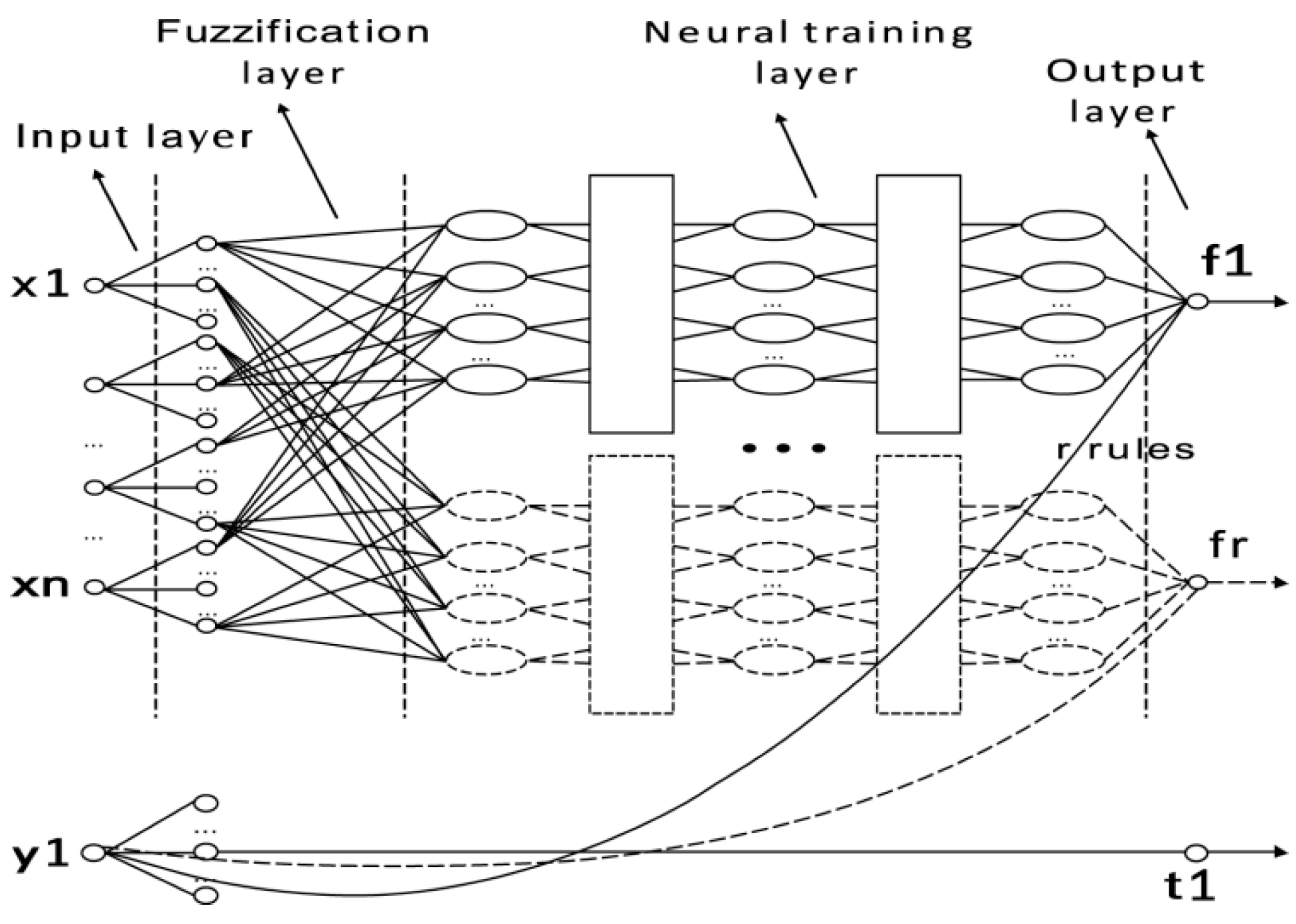
Since the sequential relation among fuzzy sets is not a direct relation among crisp numbers, now, we introduce the “fuzzy rule-based neural network” to express the fuzzy rule R_j. The theoretical structure of the fuzzy rule-based neural network (shown in Figure 2 [33]) includes Input layer, Fuzzification layer, Neural training layer and Output layer. Since there are r fuzzy rules in the fuzzy set, there are r fuzzy neural network structures in Figure 2 to match with. There may be many dashed parts, which correspond with the un-active fuzzy rules for the current training time.

Figure 2. Fuzzy rule-based neural network.

Figure 2. Fuzzy rule-based neural network.

Layer specification:

Input layer: only original (crisp) variables (x₁–x_n) are presented to this layer.

Fuzzification layer: This layer transfers the original variable values into fuzzy ones. One node of this layer mirrors one fuzzy set (Lowest, Lower, etc.) and the output link of the nodes represents the membership value, which specifies the degree of an input belongs to a fuzzy set. Then, this layer chooses the value with the maximum membership degree to participate the process of the neural training layer according to the maximum membership degree principal.

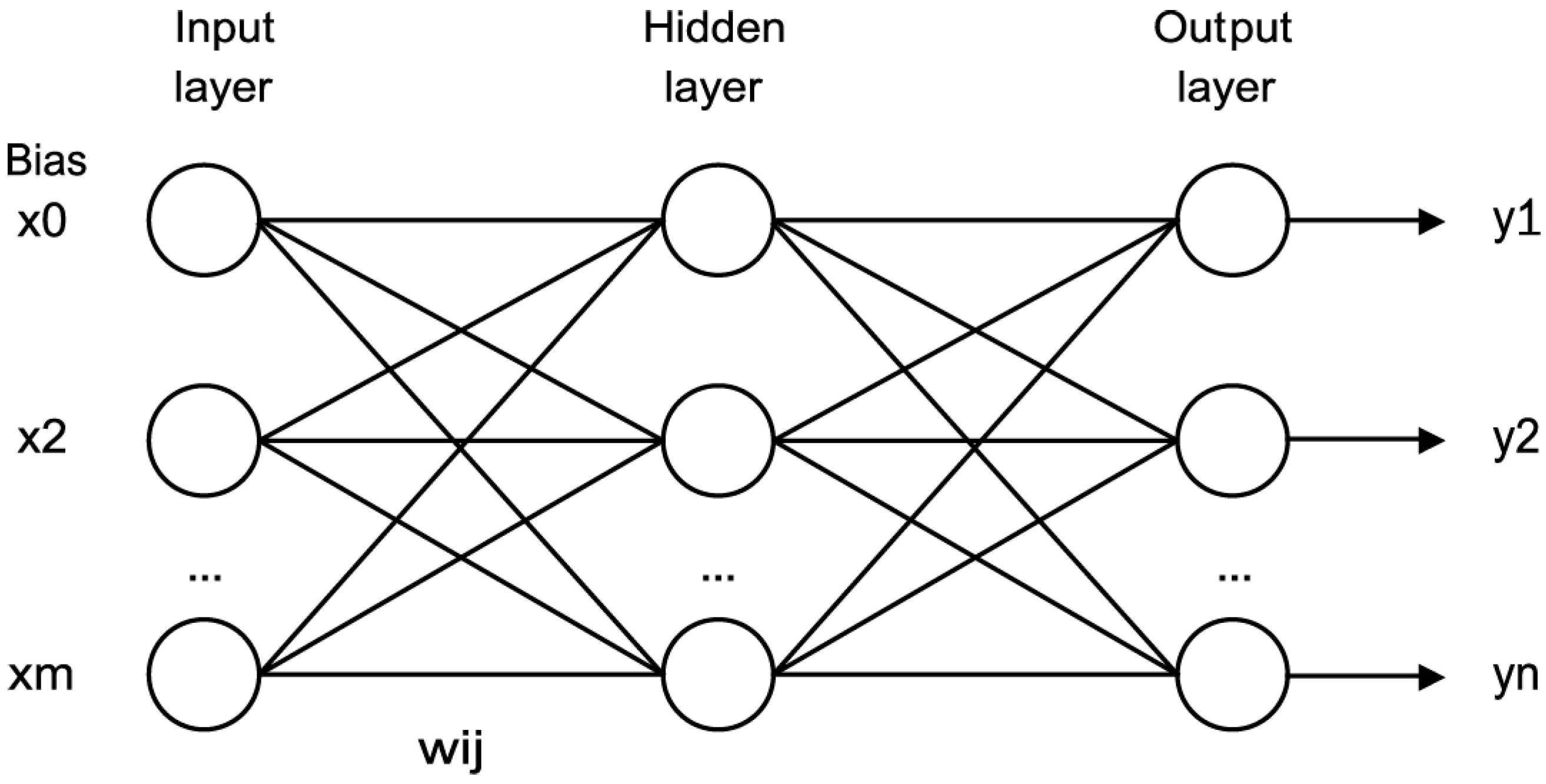
Neural training layer: This layer is the n-inputs, 1-output feed forward neural network using the BP algorithm that is commonly used. The back propagation artificial neural network (BPANN) is basically a neural network, which composed of input layer, hidden layer and the output layer [34]. Besides, it uses BP algorithm to train itself, taking inputs from the previous layer and sending outputs to the next layer. The BP algorithm determines the weights during the process of data training, resulting in a minimized error between the real and the expected values, which is used for updating the weights [35,36].

Output layer: This layer is the same to the output layer of ANNs but with a fuzzy number output.

3.2. Neural Fuzzy Inference System-Based Weather Prediction Model (NFIS-WPM)

Now we introduce the fuzzy inference system on the basis of fuzzy rule-based neural network to predict weather condition, that is, neural fuzzy inference system-based weather prediction model, NFIS-WPM for short.

3.2.1. Meteorological Fuzzy Inference System

Fuzzy inference system [33] consists of a fuzzy system with known inputs and outputs that we call “fuzzy back knowledge”; an incomplete fuzzy system with known inputs and unknown outputs that we call a “fuzzy inference problem”.

Fuzzy inference system is suited to weather forecasting, whose process is expressed by the equation:

R: G(premise) → C(conclusion)

(9)

where G(premise) contains n forecasting premises to predict C(conclusion).

Take a simple example to show how it works on a weather system. There are five forecasting premises and one meteorological element (conclusion) in the fuzzy rule set R:

• R(1): IF x₁ is X₁₁ and x₂ is X₂₁ and x₃ is X₃₁ and x₄ is X₄₁ and x₅ is X₅₁ THEN y is Y₁;
• R(2): IF x₁ is X₁₂ and x₂ is X₂₂ and x₃ is X₃₂ and x₄ is X₄₂ and x₅ is X₅₂ THEN y is Y₂;
• R(3): IF x₁ is X₁₃ and x₂ is X₂₃ and x₃ is X₃₃ and x₄ is X₄₃ and x₅ is X₅₃ THEN y is Y₃;
• R(4): IF x₁ is X₁₄ and x₂ is X₂₄ and x₃ is X₃₄ and x₄ is X₄₄ and x₅ is X₅₄ THEN y is Y₄;
• ......

If we want to deduct another rule “R(5): IF x₁ is X₁₅ and x₂ is X₂₅ and x₃ is X₃₅ and x₄ is X₄₅ and x₅ is X₅₅THEN Y is?” according to the rules above. Such problems are called “meteorological fuzzy inference problem”. X₁₁, X₁₂, X₁₃, X₁₄, ..., are different fuzzy sets.

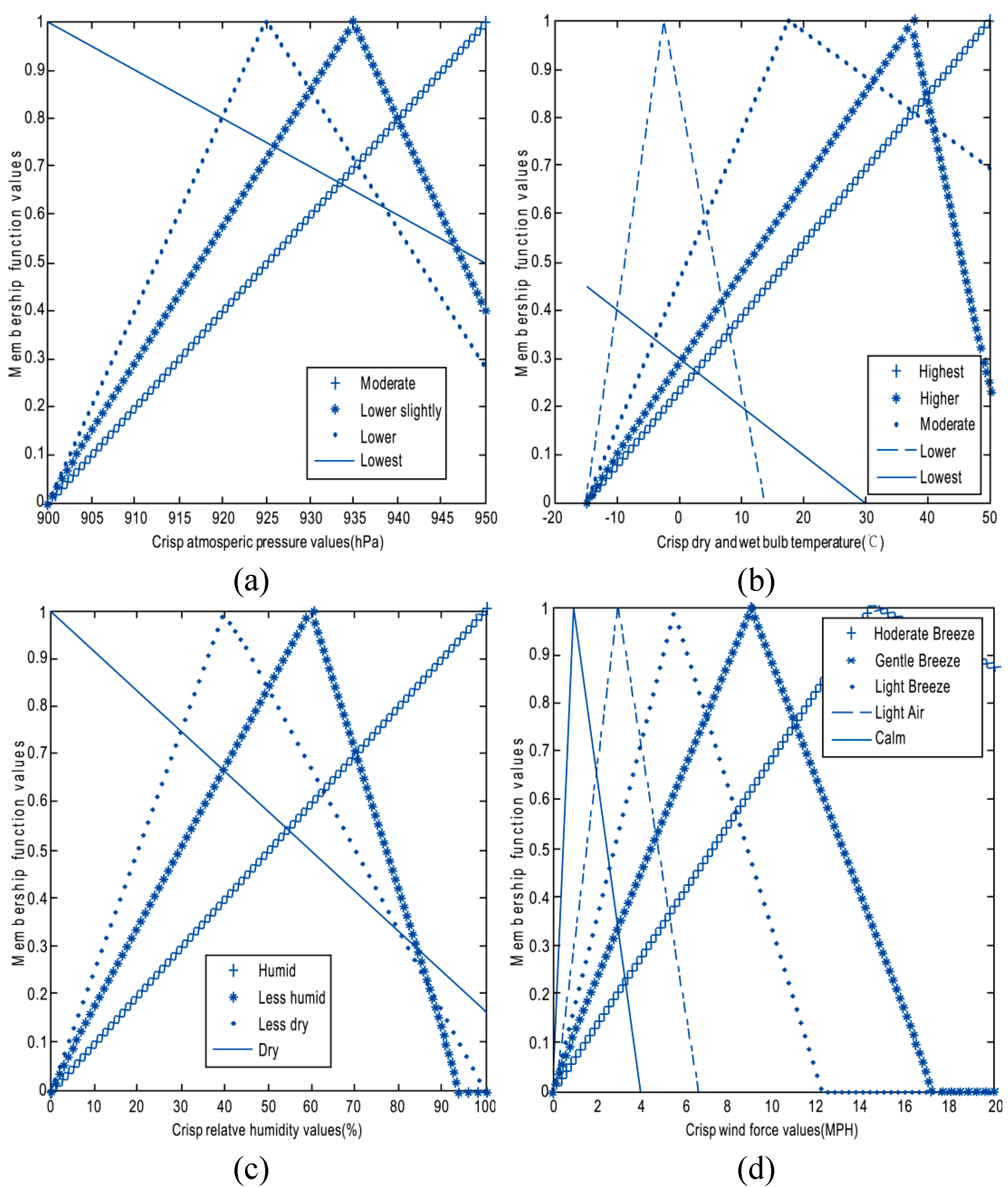
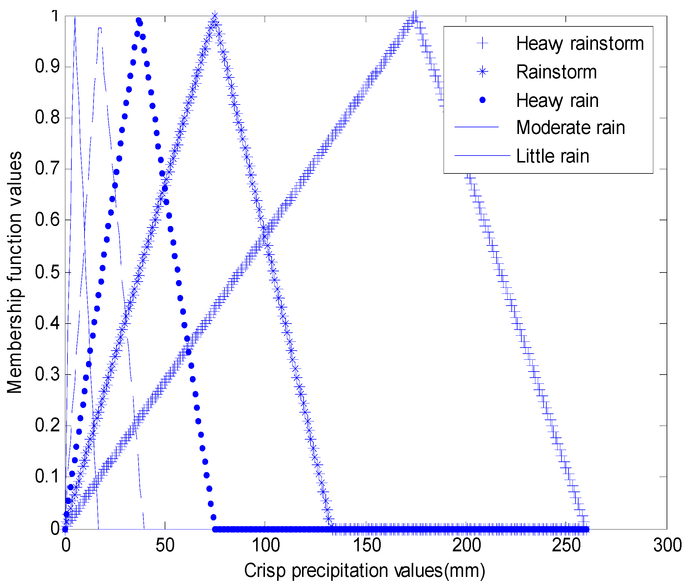
Figure 3. Membership function curves of meteorological fuzzy variable premises.

Figure 3. Membership function curves of meteorological fuzzy variable premises.

3.2.2. Meteorological Fuzzy Inference Algorithm

Meteorological fuzzy inference algorithm is the algorithm executed in the neural fuzzy inference system-based weather prediction model (NFIS-WPM)

Stage 1: In this stage, crisp numbers are mapped to corresponding fuzzy sets in accordance with the membership function curves shown in Figure 3. Now we take Figure 3a as an example to describe how we use the membership function curves to determine the corresponding fuzzy set of a crisp number. There are four membership function curves shown in this panel. Each curve is used to read the membership degrees corresponding to the atmospheric pressure values for one of the different fuzzy sets named “Lowest”, “Lower”, “Lower slightly” and “Moderate”, respectively. For example, given a crisp number “910” whose membership degree is “Moderate”, we can get the maximum membership degree value of the membership function curve for “Moderate” compared with the other three in Figure 3a, and then we map the number “910” to fuzzy set “Moderate”. Similarly, the membership function curves shown in Figure 3b–d are used to map crisp dry and wet bulb temperatures, humidity values and wind force values to corresponding fuzzy sets for temperature, humidity and wind. Thus, the training samples of ANNs are transferred into a fuzzy inference system.

Stage 2:

/* suppose there are r fuzzy rules in the rule set with the same structure and n fuzzy variables (premises) in each rule.*/

PreCount[] = 0; // set PreCount[] to zero.

for j = 1 to r for i = 1 to n if (Rnewi == Rji) PreCount[j] ++ ; end end if (PreCount[j] == n) // PreCount[j] == n when the jth fuzzy rule’s premises are the same to the new coming rule. Rnew(n+1) = Rj(n+1) end end Countj = 0 for k = 1 to r if (PreCount[j] != 0) Countj = 1; break; end end if (Countj == 0) // “Countj == 0” means the new coming rule is a new one. complexinference(); // “complexinference()” is a function related to the complex fuzzy inference. end

Stage 3: complexinference() specification

Complexinference() may contains more than one prediction model and ANN is used for simulating the process of fuzzy inference.

Void Complexinference()

for j = 1 to r /* Fuzzy rule-based neural network corresponding to Rj is used to get the membership function values of output of Rnew––Rnew(n+1), then the comparisonbetween the output and each fuzzy set of the restricted domain is made*/ if (the output is consistent with some fuzzy set of the restricted domain to a certain degree β or bigger than β) output the fuzzy set else choose the fuzzy set with the most similarities end end /* “restricted domain” refers to the range of the output we set in advance. If we hope to restrict the range of the output to {Higher, High, Lower, Low }, the restricted domain is {Higher, High, Lower, Low}. β is a threshold to control the similarity degree of the output and the element of the restricted domain.*/

In mathematics, a function is a relation between inputs and outputs with the property that each unique combination of inputs matches with exactly one output. An example is the function that relates each real number μ_A(x) to μ_B(x). In this example, if the inputs μ_A(3) = μ_A(4) and the output are 0.9 and 0.8, respectively, then we say the relation between μ_A(x) to μ_B(x) is not a function since the same input values lead to different output values. Similarly, our model is a relation between the fuzzy variable inputs and a set of fuzzy variable output. After completing the whole process, the same meteorological premises may lead to different meteorological conclusions.

To solve such problem, we introduce the concept of the expected value (Definition 3.1):

Definition 3.1 Let X be a discrete random variable taking numerical values with distribution function p(x). The expected value E(X) is defined as:

$$E(X)={\sum }_{x\in \text{Ω}}xp\left(x\right)$$

(10)

The expected value is a weighted average of all possible values, each of which is multiplied by its assigned distribution function, and the final products are then added together to get the expected value. Obviously, the values used to calculate the expected value should be numerical, but our model’s value is a fuzzy set, in other words, linguistic. To solve this problem, we use a number to represent a linguistic variable value, for example, use “1” to replace “Little rain”. NFIS-WPM combing the method described above is called NFIS-WPM (Ave). We should notice that the hitting rate (Definition 3.2) in NFIS-WPM (Ave) would drop down sharply since the expected value is a compromise among the different possible outputs.

Definition 3.2 Let Correctp be times of correct prediction and overall times of prediction as Totalp. The hitting rate Hitrate is defined as:

Hitrate = Correctp/Totalp

(11)

Under these circumstances, we adopt the policy of rounding up. For example, if “1” is to represent “Little rain” and “2” is to represent “Moderate rain” and there is a number “1.6”, so we give the prediction result as “Moderate rain”.

Or we just give the value with the highest possibility among all the generated values to the fuzzy variable. This is a more straight-forward method. Similarly, NFIS-WPM combing this method is called NFIS-WPM (Hig-prob).

4. Experiments and Analysis

4.1. Data Collection

The surface meteorological observation data used in this experiment were collected from the Shanxi Provincial Meteorological Bureau, China. The day’s wind speed, dry and wet bulb temperature, relative humidity, atmospheric pressure and accumulated precipitation at 20 o’clock (Beijing Time) in Taiyuan, Shanxi, China from May 2010 to October 2010, May 2011 to October 2011 and May 2012 to October 2012 were selected. We also got the Global Ensemble Forecast System (GEFS) product data for comparison from the Environmental Modeling Center, National Centers for Environmental Prediction, USA.

4.2. Experimental Section

The NFIS-WPM, NFIS-WPM (Ave) and NFIS-WPM (Hig-prob) are tested in this experiment, and a traditional ANN weather prediction model is used for comparison. The day’s wind speed, dry and wet bulb temperature, relative humidity, and atmospheric pressure observations at 20 o’clock (Beijing Time) are taken as inputs while the accumulated precipitation for the next 24 h is taken as outputs for the weather prediction models. The precipitation observations are used to verify the model prediction results.

Atmospheric pressure falls into four fuzzy sets in Table 1; relative humidity falls into four fuzzy sets shown in Table 2; dry and wet bulb temperature falls into five fuzzy sets shown in Table 3; wind speed falls into five categories (fuzzy sets) shown in Table 4; precipitation falls into five fuzzy sets shown in Table 5. In order to test NFIS-WPM (Ave), numbers from 0 to 4 inclusively are given to represent No rain, Light rain, Moderate rain, Heavy rain and Rainstorm, respectively (Figure 4) [37,38,39].

Table 1. Fuzzy classification of atmospheric pressure.

Atmospheric Pressure Rating	Moderate	Lower Slightly	Lower	Lowest
Atmospheric pressure value (hPa)	>940	[930, 940]	[920, 930)	<920

Table 1. Fuzzy classification of atmospheric pressure.

Atmospheric Pressure Rating	Moderate	Lower Slightly	Lower	Lowest
Atmospheric pressure value (hPa)	>940	[930, 940]	[920, 930)	<920

Table 2. Fuzzy classification of dry and wet bulb temperature.

Dry and Wet Bulb Temperature Rating	Lowest	Lower	Moderate	Higher	Highest
Dry and wet bulb temperature value (°C)	<−10	[−10, 5)	[5, 30)	[30, 45]	>45

Table 2. Fuzzy classification of dry and wet bulb temperature.

Dry and Wet Bulb Temperature Rating	Lowest	Lower	Moderate	Higher	Highest
Dry and wet bulb temperature value (°C)	<−10	[−10, 5)	[5, 30)	[30, 45]	>45

Table 3. Fuzzy classification of relative humidity.

Relative Humidity Rating	Dry	Less Dry	Less Humid	Humid
Relative humidity value (%)	[0, 30)	[30, 50)	[50, 70)	[70, 100]

Table 3. Fuzzy classification of relative humidity.

Relative Humidity Rating	Dry	Less Dry	Less Humid	Humid
Relative humidity value (%)	[0, 30)	[30, 50)	[50, 70)	[70, 100]

Table 4. Fuzzy classification of wind speed.

Wind Speed Rating	Calm	Light Air	Light Breeze	Gentle Breeze	Moderate Breeze
Wind speed value (MPH)	(0, 2)	[2, 4)	[4, 7)	[7, 11)	[11, 17)

Table 4. Fuzzy classification of wind speed.

Wind Speed Rating	Calm	Light Air	Light Breeze	Gentle Breeze	Moderate Breeze
Wind speed value (MPH)	(0, 2)	[2, 4)	[4, 7)	[7, 11)	[11, 17)

Table 5. Fuzzy classification of precipitation.

Precipitation Rating	No Rain	Light Rain	Moderate Rain	Heavy Rain	Rainstorm
Precipitation value (mm)	0	(0, 10)	[10, 25)	[25, 50)	[50, +∞)

Table 5. Fuzzy classification of precipitation.

Precipitation Rating	No Rain	Light Rain	Moderate Rain	Heavy Rain	Rainstorm
Precipitation value (mm)	0	(0, 10)	[10, 25)	[25, 50)	[50, +∞)

Figure 4. Membership function curves of meteorological fuzzy variable output.

Figure 4. Membership function curves of meteorological fuzzy variable output.

4.3. Experiment Results and Error Analysis

Results from Figure 5, Figure 6, Figure 7, Figure 8, Figure 9 and Table 6 indicate:

(1) ANNs are used to predict the exact precipitation for weather forecasting, but lead to the non-accuracy of the prediction outputs. Hitting rate is 0, which means that the rate of prediction accuracy is 0. Figure 5 shows that ANNs never accurately forecasted strong rainfalls whose precipitations were more than 20 mm during the experimental time period. However, it had forecasted rainfalls in the non-rainfall days during the experiment. Therefore, we believe that ANNs are almost impossible to forecast precipitation.

(2) NFIS-WPM is not good enough to get an accurate result. Figure 5 shows that it often made mistakes in predicting precipitation, especially when the actual precipitation was light, which was often erroneously forecasted as a heavy precipitation. Hitting rate is only 0.18, just a little bit better than ANNs. The same meteorological premises may lead to several different conclusions in NFIS-WPM; we just randomly choose one of the possible fuzzy sets. It is the randomness that leads to this accuracy.

(3) NFIS-WPM (High Pro) is the improvement of NFIS-WPM. There is a significant change in average error, from 1.54 levels to 0.36 levels; and plenty of raises in hitting rate, from 0.18 to 0.73. However, the biggest disadvantage of NFIS-WPM (High Pro) is its tendency to obtain false negatives.

(4) NFIS-WPM (Ave) is another improvement of NFIS-WPM. Figure 8 shows that NFIS-WPM (Ave) has the best performance in predicting moderate rainfall. Table 6 shows that the NFIS-WPM (Ave) is a relatively stable model since the errors fall within an interval between 0 and 1.56 levels and its hitting rate is the best of the four methods. However, the predicted precipitation level is increased, but quite stable compare with the actual variability of precipitation, since we just give the value with the average possibility among all the generated values to the fuzzy variable, and it will weaken the extreme values forecast.

(5) We compared the precipitation predicting results of our NFIS-WPM (Ave) with the existing operational prediction system, the GEFS ensemble mean shown in Figure 9. GEFS ensemble mean leads to a lower accuracy with the hitting rate of 0.31. After the comparison, we believe that our NFIS-WPM (Ave) performs better than the GEFS ensemble mean in forecasting precipitation.

Figure 5. Testing results of artificial neural network (ANN).

Figure 5. Testing results of artificial neural network (ANN).

Figure 6. Testing results of NFIS-WPM.

Figure 6. Testing results of NFIS-WPM.

Figure 7. Testing results of NFIS-WPM (High-prob).

Figure 7. Testing results of NFIS-WPM (High-prob).

Figure 8. Testing results of NFIS-WPM (Ave).

Figure 8. Testing results of NFIS-WPM (Ave).

Figure 9. Evaluation of GEFS ensemble mean.

Figure 9. Evaluation of GEFS ensemble mean.

Table 6. Comparison between ANN and neural fuzzy inference system-based weather prediction model.

	Minimum Error	Maximum Error	|Minimum Error|	|Maximum Error|	Average |Error|	Hit Rate
ANN	−60.6 mm	4.42mm	0.01 mm	60.6 mm	3.42 mm	0
NFIS-WPM	−1 level	4 level	0 level	4 level	1.54 level	0.18
NFIS-WPM (High-prob)	−4 level	1 level	0 level	4 level	0.36 level	0.73
NFIS-WPM (Ave)	0 level	1.56 level	0 level	1.56 level	0.77 level	0.75
GEFS	−91.4 mm	35.5mm	0.00 mm	91.4 mm	4.83 mm	0.31

Table 6. Comparison between ANN and neural fuzzy inference system-based weather prediction model.

	Minimum Error	Maximum Error	|Minimum Error|	|Maximum Error|	Average |Error|	Hit Rate
ANN	−60.6 mm	4.42mm	0.01 mm	60.6 mm	3.42 mm	0
NFIS-WPM	−1 level	4 level	0 level	4 level	1.54 level	0.18
NFIS-WPM (High-prob)	−4 level	1 level	0 level	4 level	0.36 level	0.73
NFIS-WPM (Ave)	0 level	1.56 level	0 level	1.56 level	0.77 level	0.75
GEFS	−91.4 mm	35.5mm	0.00 mm	91.4 mm	4.83 mm	0.31

5. Discussion and Conclusions

In this paper, the crisp inputs of the neural network are changed into fuzzy ones; correspondingly, the structure of the neural network is also changed. Then, specific models based on the improved neural network are used to predict weather conditions such as precipitation and get a better result than the traditional neural network. In particular, NFIS-WPM (High Pro) and NFIS-WPM (Ave) can reduce the prediction error significantly in precipitation and increase the hitting rate greatly compared with traditional ANNs.

It is well known that the need for accurate weather prediction is apparent when considering the benefits that it has. However, after Lorenz’s work on Chaos Theory in the 1960s [40], probabilistic predictions have gradually dominated weather and forecasting. A recent study [41] shows how Lorenz’s theory influences the ways in which we seek to represent uncertainty in forecasting. In addition, precipitation change due to global warming is highly uncertain, which has a profound impact on the human living environment [42]. Therefore, “uncertainty” should be considered under the challenges posed by climate change and represented in weather prediction systems such as probabilistic or fuzzy forecasting. Atmospheric motion is uncertain, and it is fuzzy [43,44]; that means the “accuracy” in weather prediction using neural networks with crisp premises makes some of the accurate prediction results useless and meaningless, since sometimes the meaningful relation among different objects only exists when the premises are treated as fuzzy variables. By adapting this novel model to the weather prediction problem, we reduce the “uncertainty” in weather prediction since inputs of the neural network we propose in our paper are fuzzy sets, which mean a sort of “uncertainty”. Furthermore, it is these “sort of uncertainty inputs” that make the outcomes of the weather prediction more meaningful and accurate [45].

The neural fuzzy inference system-based weather prediction model is one of the data driven modeling approaches. The problem with the data driven modeling approach is that the underlying rules cannot be specified [46,47]. Thus, data driven modeling may provide a practical or feasible way to solve problems worldwide. The computing world has a lot to gain from neural networks. Their greatest advantage is their ability to model complicated non-linear relationships without a priori assumptions, just like a black box [48]. They have the ability to learn through examples, making them very flexible and powerful. Furthermore, there is no need to know the internal mechanisms of a task. The obtained results also showed that NFIS-WPMs outperformed the ANNs models. This may be related to the effect of fuzzification for the inputs through fuzzy classification methods. Because the meteorological premises were first fuzzified and then fed to the NFIS-WPMs, and fuzzy-based neural network modeling has been performed on the fuzzified data, the ability of these modeling approaches has been improved.

As we know, weather forecasting methods are often comprehensive since a single method or model may be unable to get good results [49,50,51]; this is because the atmosphere has nonlinear movement. Atmospheric flows are usually described by a system of nonlinear partial differential equations. Within this framework, we should not only consider the stochastically forced dynamical system, but also consider observations as the stochastic process rather than single numerical values [52]. Thus, this makes numerical weather prediction models based on atmospheric dynamics equations and physical process parameterization theories increasingly complex and difficult to manage. However, our models that have the ability to model complex nonlinear relationships could reduce the prediction error by large amounts. What we should notice is that neural network predicts future results based on previous experience. However, future weather conditions do not always relate to the previous status. In this case, our system cannot get meaningful prediction outcomes. Besides, our system has to learn before predicting, if there is no old information available, we cannot use this prediction system.

There are a lot of types of ANNs and our system is based on BP-backward neural networks. We may replace the core part of our prediction system with another type of neural network and it may be able to get better predictive results than the system proposed in this article. Or we can just use our system to test the other meteorological elements as well. However, scope is lacking for a detailed description of it.

References

1. Matbouli, Y.T.; Hipel, K.W.; Kilgour, D.M.; Karray, F. A fuzzy logic approach to assess, manage, and communicate carcinogenic risk. Hum. Ecol. Risk Assess. 2014, 20, 1687–1707. [Google Scholar] [CrossRef]
2. Precup, R.E.; Tomescu, M.L.; Dragos, C.A. Stabilization of Rössler chaotic dynamical system using fuzzy logic control algorithm. Int. J. Gen. Syst. 2014, 43, 413–433. [Google Scholar] [CrossRef]
3. Roman-Flores, H.; Barros, L.C.; Bassanezi, R.C. A note on Zadeh’s extensions. Fuzzy Sets Syst. 2001, 117, 327–331. [Google Scholar] [CrossRef]
4. Stotts, L.; Brian, H.K. New developments in fuzzy logic computers. Ind. Manag. Data Syst. 1995, 95, 13–17. [Google Scholar] [CrossRef]
5. Charan, T.G.; Kalyani, V.K.; Sharma, K.K.; Kumar, L.; Kumari, S.; Sinha, A. Use of an artificial neural network to evaluate the oleo-flotation process to treat coal fines. Int. J. Coal Prep. Util. 2014, 34, 229–238. [Google Scholar] [CrossRef]
6. Fakhri, M.; Ghanizadeh, A.R. Modelling of 3D response pulse at the bottom of asphalt layer using a novel function and artificial neural network. Int. J. Pavement Eng. 2014, 15, 671–688. [Google Scholar] [CrossRef]
7. Andrew, A.M. Artificial neural nets and BCL. Kybernetes 2005, 34, 33–39. [Google Scholar] [CrossRef]
8. González, J.M.B.; Des Jardins, S.L. Artificial neural networks: A new approach to predicting application behavior. Res. High. Educ. 2002, 43, 235–258. [Google Scholar] [CrossRef]
9. Karakis, R.; Capraz, I.; Bilir, E.; Guler, I. EEG source localization using a genetic algorithm-based artificial neural network. Recent Pat. Biomed. Eng. 2013, 6, 188–194. [Google Scholar] [CrossRef]
10. Jiang, C.; Huang, H.S. Patent review on network-based elderly healthcare system in the US. Recent Pat. Comput. Sci. 2013, 6, 181–190. [Google Scholar] [CrossRef]
11. Li, S.; Wu, Z. Business performance forecasting of convenience store based on enhanced fuzzy neural Network. Neural Comput. Appl. 2008, 17, 569–578. [Google Scholar] [CrossRef]
12. Rajasekaran, S.; Febin, M.F.; Ramasamy, J.V. Artificial fuzzy neural network in civil engineering. Comput. Struct. 1996, 61, 291–302. [Google Scholar] [CrossRef]
13. Soria-Olivas, E.; Martin-Guerrero, J.D. A low complexity fuzzy activation function for artificial neural networks. IEEE Trans. Neural Netw. 2003, 14, 1576–1589. [Google Scholar] [CrossRef] [PubMed]
14. Hsieh, K.L. Process improvement in the presence of qualitative response by combining fuzzy sets and neural networks. Integr. Manuf. Syst. 2001, 12, 449–462. [Google Scholar] [CrossRef]
15. Baghaee, M.; Shahbazian, M. Modeling the permeability of a reservoir using a new hybrid fuzzy-neural network strategy. Energy Sources 2013, 35, 1000–1006. [Google Scholar] [CrossRef]
16. Li, W. A method for design of a hybrid neuro-fuzzy control system based on behavior modeling. IEEE Trans. Fuzzy Syst. 1997, 5, 462–477. [Google Scholar]
17. Meng, X.M. Weather forecast based on improved genetic algorithm and neural network. Lect. Notes Electr. Eng. 2013, 219, 833–838. [Google Scholar]
18. Masinde, M. Artificial neural networks models for predicting effective drought index: Factoring effects of rainfall variability. Mitig. Adapt. Strateg. Glob. Change 2013. [Google Scholar] [CrossRef]
19. Nayak, R.; Patheja, P.S.; Waoo, A. An enhanced approach for weather forecasting using neural network. Adv. Intell. Soft Comput. 2012, 131, 833–839. [Google Scholar]
20. Alessandro, B.; Fátima, A.M.; Roberto, G. Ground-level ozone prediction using a neural network model based on meteorological variables and applied to the metropolitan area of São Paulo. Int. J. Environ. Pollut. 2012, 49, 1–15. [Google Scholar] [CrossRef]
21. Grinn-Gofron, A.; Strzelczak, A. Artificial neural network models of relationships between cladosporium spores and meteorological factors in Szczecin (Poland). Grana 2008, 47, 305–315. [Google Scholar] [CrossRef]
22. Dorvlo, A.S.S.; Jervase, J.A.; AI-Lawati, A. Solar radiation estimation using artificial neural networks. Appl. Energy 2002, 71, 307–319. [Google Scholar] [CrossRef]
23. Potts, V.L.; Miima, B.J.; Acar, M. Course evaluation using fuzzy linguistic rules. Surv. Land Inf. Sci. 2012, 72, 119–128. [Google Scholar]
24. Zadeh, L.A. The concept of a linguistic variable and its application to approximate reasoning, Part I. Inf. Sci. 1975, 8, 199–249. [Google Scholar] [CrossRef]
25. Kissi, M.; Ramdani, M.; Tollabi, M.; Zakarya, D. Determination of fuzzy logic membership functions using genetic algorithms: Application to structure-odor modeling. J. Mol. Model. 2004, 10, 335–341. [Google Scholar] [CrossRef] [PubMed]
26. Grauel, A.; Ludwig, L.A. Construction of differentiable membership functions. Fuzzy Sets Syst. 1999, 101, 219–225. [Google Scholar] [CrossRef]
27. Guresen, E.; Kayakutlu., G.; Daim, T.U. Using artificial neural network models in stock market index prediction. Expert Syst. Appl. 2011, 38, 10389–10397. [Google Scholar] [CrossRef]
28. Bahrammirzaee, A. A comparative survey of artificial intelligence applications in finance: Artificial neural networks, expert system and hybrid intelligent systems. Neural Comput. Appl. 2010, 19, 1165–1195. [Google Scholar] [CrossRef]
29. Amjady, N.; Keynia, F. A new neural network approach to short term load forecasting of electrical power systems. Energies 2011, 4, 488–503. [Google Scholar] [CrossRef]
30. Chen, Y.; Luh, P.B.; Guan, C.; Zhao, Y.; Michel, L.D.; Coolbeth, M.A.; Friedland, P.B.; Rourke, S.J. Short-term load forecasting: Similar day-based wavelet neural networks. IEEE Trans. Power Syst. 2010, 25, 322–330. [Google Scholar] [CrossRef]
31. Tengeleng, S.; Armand, N. Performance of using cascade forward back propagation neural networks for estimating rain parameters with rain drop size distribution. Atmosphere 2014, 5, 454–472. [Google Scholar] [CrossRef]
32. Shanmuganathan, S.; Sallis, P. Data mining methods to generate severe wind gust models. Atmosphere 2014, 5, 60–80. [Google Scholar] [CrossRef] [Green Version]
33. Lu, J. A neural fuzzy inference system. J. Electron. China 2013, 30, 401–410. [Google Scholar]
34. Prasad, R.; Pandey, A.; Singh, K.P.; Singh, V.P.; Mishra, R.K.; Singh, D. Retrieval of spinach crop parameters by microwave remote sensing with back propagation artificial neural networks: A comparison of different transfer functions. Adv. Space Res. 2012, 50, 363–370. [Google Scholar] [CrossRef]
35. Wang, J.Z.; Wang, J.J.; Zhang, Z.G.; Guo, S.P. Forecasting stock indices with back propagation neural network. Expert Syst. Appl. 2011, 38, 14346–14355. [Google Scholar]
36. Wang, Y.H. Nonlinear neural network forecasting model for stock index option price: Hybrid GJR-GARCH approach. Expert Syst. Appl. 2009, 36, 564–570. [Google Scholar] [CrossRef]
37. Kwarteng, A.Y.; Dorvlo, A.S.; Vijaya Kumar, G.T. Analysis of a 27-year rainfall data (1977–2003) in the Sultanate of Oman. Int. J. Climatol. 2009, 29, 605–617. [Google Scholar] [CrossRef]
38. Ding, G.; Gao, L.; Li, X.; Zhou, M.; Liu, Q.; Ren, H.; Jiang, B. A mixed method to evaluate burden of Malaria due to flooding and water logging in Mengcheng County, China: A case study. PLoS One 2014. [Google Scholar] [CrossRef]
39. Qian, W.; Fu, J.; Yan, Z. Decrease of light rain events in summer associated with a warming environment in China during 1961–2005. Geophys. Res. Lett. 2007. [Google Scholar] [CrossRef]
40. Lorenz, E.N. Energy and numerical weather prediction. Tellus 1960, 12, 364–373. [Google Scholar] [CrossRef]
41. Slingo, J.; Palmer, T. Uncertainty in weather and climate prediction. Phil. Trans. R. Soc. 2011, 369, 4751–4767. [Google Scholar] [CrossRef]
42. Ma, J.; Xie, S.P. Regional patterns of sea surface temperature change: A source of uncertainty in future projections of precipitation and atmospheric circulation. J. Clim. 2013, 26, 2482–2501. [Google Scholar] [CrossRef]
43. Lin, J.C.; Brunner, D.; Gerbig, C. Studying atmospheric transport through Lagrangian models. EOS Trans. Am. Geophys. Union 2011, 92, 177–178. [Google Scholar] [CrossRef]
44. Williams, J.L.; Maxwell, R.M. Propagating subsurface uncertainty to the atmosphere using fully coupled stochastic simulations. J. Hydrometeorol. 2011, 12, 690–701. [Google Scholar] [CrossRef]
45. Demirel, M.C.; Booij, M.J.; Hoekstra, A.Y. The skill of seasonal ensemble low flow forecasts for four different hydrological models. Hydrol. Earth Syst. Sci. Discuss. 2014, 11, 5377–5420. [Google Scholar] [CrossRef]
46. Moraga, C. Data driven fuzzy modelling with neural networks. Stud. Fuzziness Soft Comput. 2005, 179, 153–164. [Google Scholar]
47. Kjaerulff, U.B.; Madsen, A.L. Bayesian Networks and Influence Diagrams: A Guide to Construction and Analysis, 1st ed.; Springer: New York, NY, USA, 2008. [Google Scholar]
48. Shirmohammadi, B.; Vafakhah, M.; Moosavi, V.; Moghaddamnia, A. Application of several data-driven techniques for predicting groundwater level. Water Resour. Manag. 2013, 27, 419–432. [Google Scholar] [CrossRef]
49. Jin, L.; Kong, F.; Lei, H.; Hu, Z. A methodological study on using weather research and forecasting (WRF) model outputs to drive a one-dimensional cloud model. Adv. Atmos. Sci. 2014, 31, 230–240. [Google Scholar] [CrossRef]
50. Ringelband, T.; Schäfer, R.; Moser, A. Probabilistic ampacity forecasting for overhead lines using weather forecast ensembles. Electr. Eng. 2013, 95, 99–107. [Google Scholar] [CrossRef]
51. Leu, J.S.; Su, K.W.; Chen, C.T. Ambient mesoscale weather forecasting system featuring mobile augmented reality. Multimed. Tools Appl. 2013. [Google Scholar] [CrossRef]
52. Tang, Y.M.; Ambandan, J.; Chen, D.K. Nonlinear measurement function in the ensemble Kalman Filter. Adv. Atmos. Sci. 2014, 31, 551–558. [Google Scholar] [CrossRef]