3.1. Carbon Monoxide
Combustion of hydrocarbons in a limited supply of oxygen produces carbon monoxide, a colorless, odorless, toxic gas. In Mexico, CO emitted from vehicles is the principal source of carbon monoxide, accounting for 91.8% of the total (38,521 kton/year) in 2005 [
27]. Monthly average concentrations of CO in the MCMA, GMA, and MMA over the study period are shown in
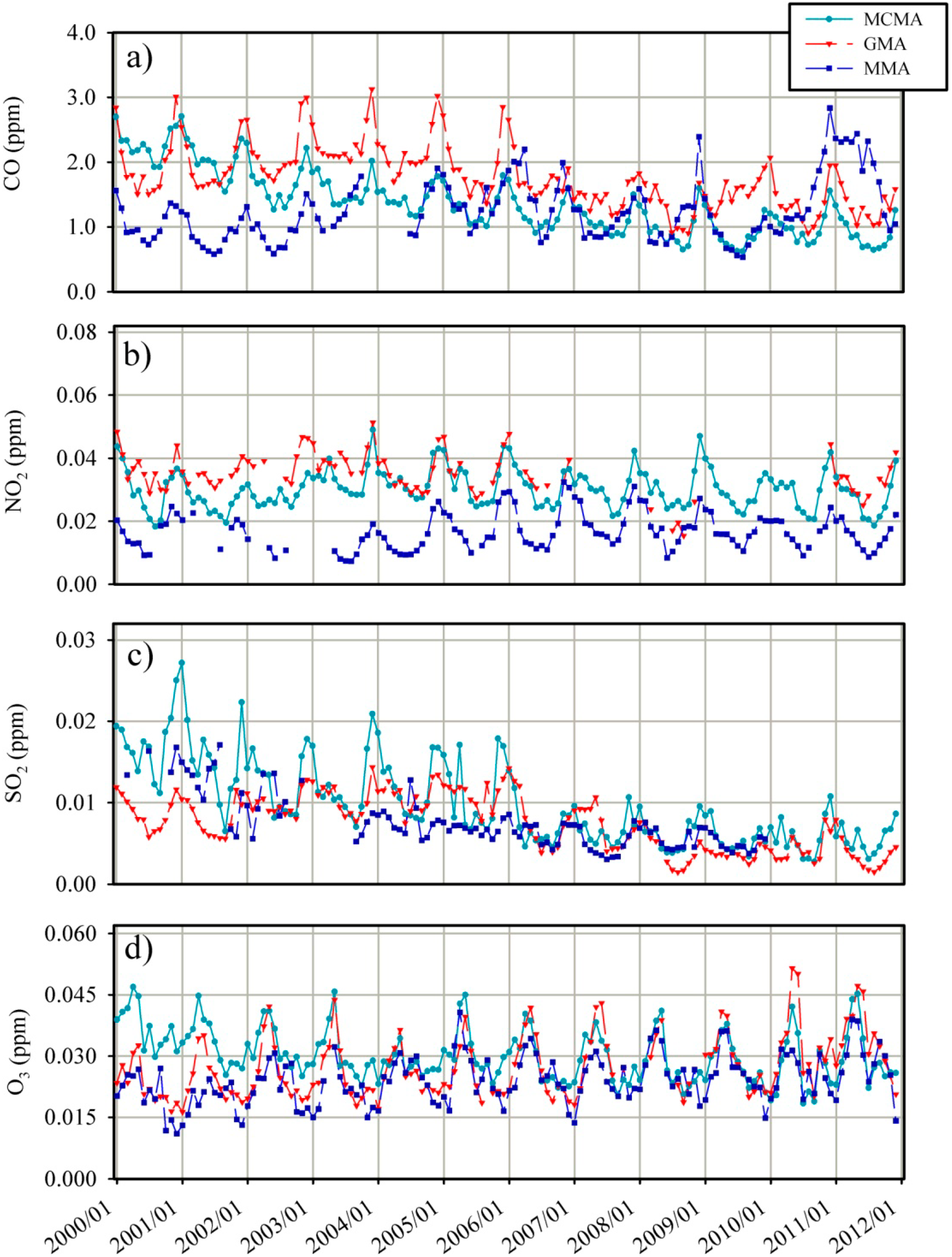
Figure 2a. In all study areas, high concentrations of CO were present during the dry-cold season, because strong atmospheric stability suppressed dilution of pollutants, particularly in the morning rush hours. Low concentrations were observed in the rainy season, when mixing in the boundary layer was vigorous.
Figure 2.
Variation of the monthly average concentrations of (a) CO, (b) NO2, (c) SO2, and (d) O3 in the three Mexican metropolitan areas from 2000 to 2011.
Figure 2.
Variation of the monthly average concentrations of (a) CO, (b) NO2, (c) SO2, and (d) O3 in the three Mexican metropolitan areas from 2000 to 2011.
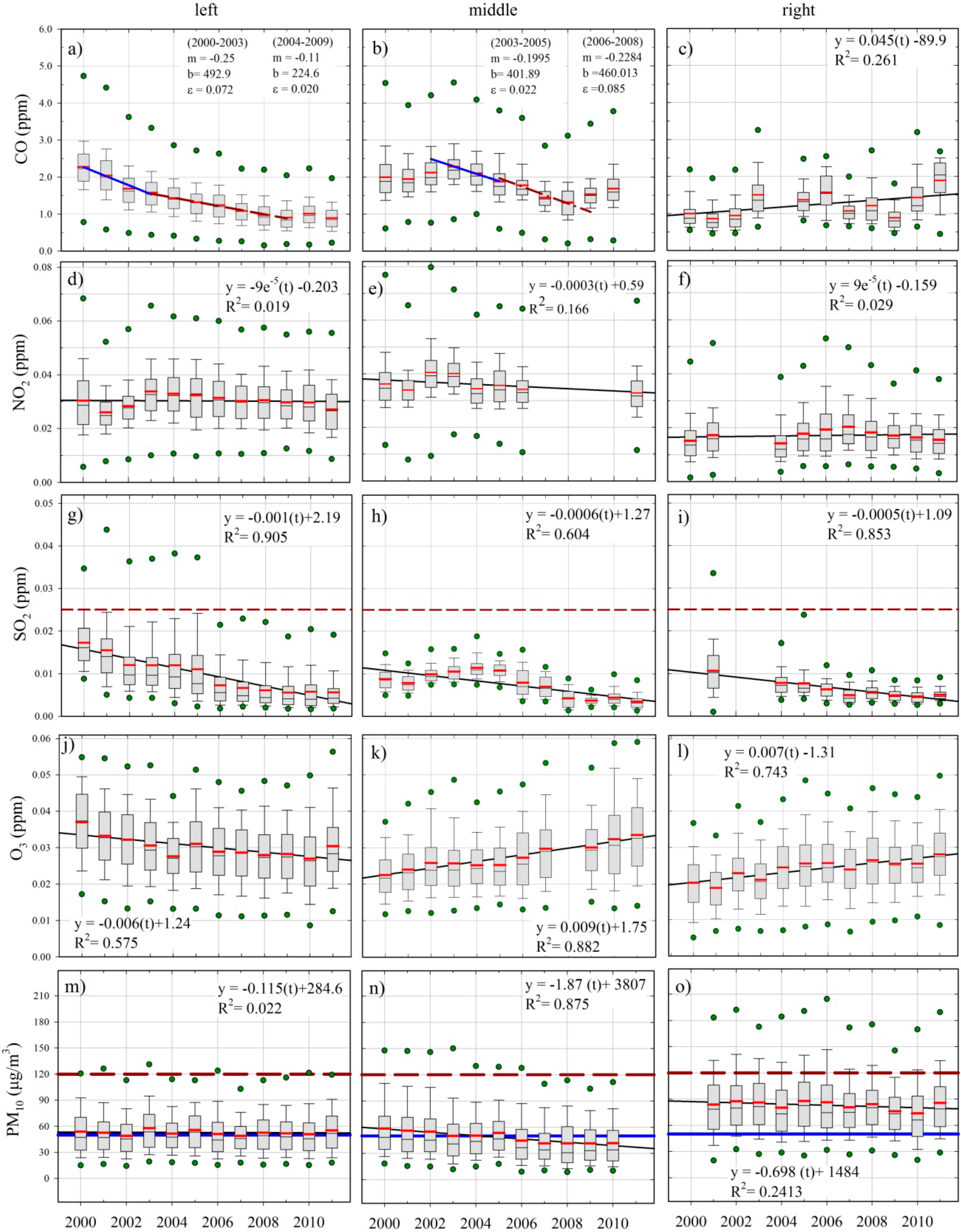
Figure 3a–c show trends for the annual mean concentration of CO in the MCMA, GMA, and MMA, respectively. In Mexico, in 2006, NOM-041-SEMARNAT-2006 (which defined limits of pollutant emissions from mobile sources) was issued and various actions were implemented in federal and local governments. By 2013, 16 Mexican states had programs for certification of vehicular emission, but only in 12 states (including Mexico state and DF in the MCMA) were the programs mandatory; in other areas such as the GMA and MMA, the fulfillment of the norm was a choice of the individuals without penalty [
20].
Figure 3.
Trends for annual mean concentrations of CO, NO
2, SO
2, O
3, and PM
10 in the (
left) Mexico City Metropolitan area (MCMA), (
middle) Guadalajara Metropolitan area (GMA), and (
right) Monterrey Metropolitan area (MMA). The panels show the mean (red line), median (black line), and the 2nd to 98th (green circles), 10th to 90th (bars), and 25th to 75th (gray boxes) percentiles of daily averaged concentrations. The dashed red and solid blue lines show the levels of the corresponding air quality standard in Mexico for SO
2 and PM
10 (see
Table 2).
In (a) and (b) m, b and ε represent the value of the slope, intercept and standard error respectively, from the regression analysis for the indicate period of time.
In understanding the trends of CO concentration, characteristics of vehicle fleet are important.
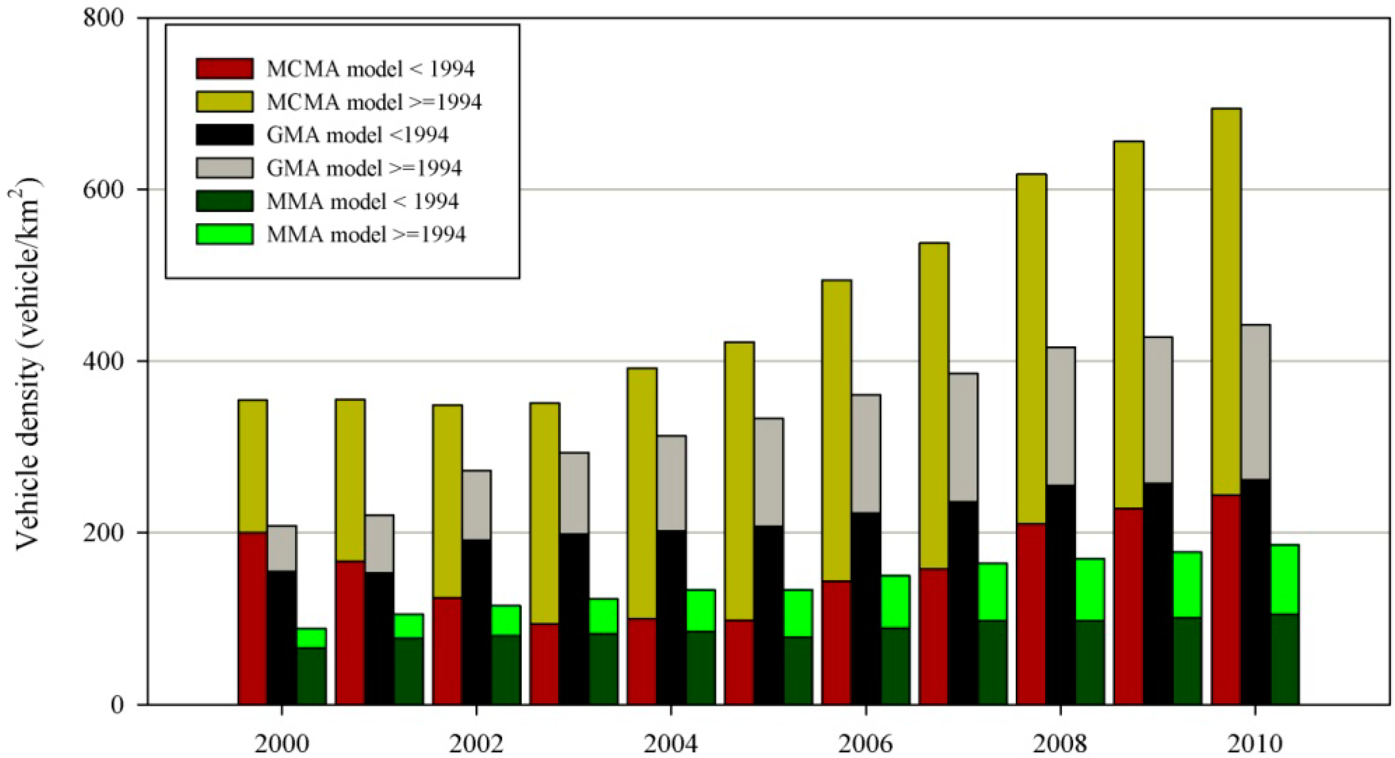
Figure 4 shows the number density of vehicles of model year older than 1994, and newer than or equal to 1994. The model-year division at 1994 has significance in that three-way catalytic converters with closed-loop controls were introduced on private vehicles in 1993, resulting in much smaller CO emission factors, 2.11 g/km estimated for 1993 and newer models (EF
MC_n) compared to >7 g/km for older models (EF
MC_o) [
28].
A reduction of ~61% in the annual mean concentration of CO in the MCMA from 2000 (2.28 ppm) to 2011 (0.88 ppm) was partly due to the improvement in the public transportation system (subway, trolley bus and metrobus) and the replacement of buses conducted as part of the PROAIRE 2002–2010 air quality management program. Other actions of PROAIRE were the modification of the threshold of emission of pollutants from vehicular sources in the MCMA, in which the threshold was reduced to about a third of the values for other urban areas determined in 1999 (NOM-041-SEMARNAT-2006).
To evaluate the influence of such actions in the MCMA, two periods were analyzed: 2000–2003 and 2004–2009 (
Figure 3a). In the first period, the number of vehicles remained almost constant, but replacement of older models with newer models equipped with catalytic converters proceeded rapidly, whereas in the second period, the number of vehicles increased for both older and newer models (
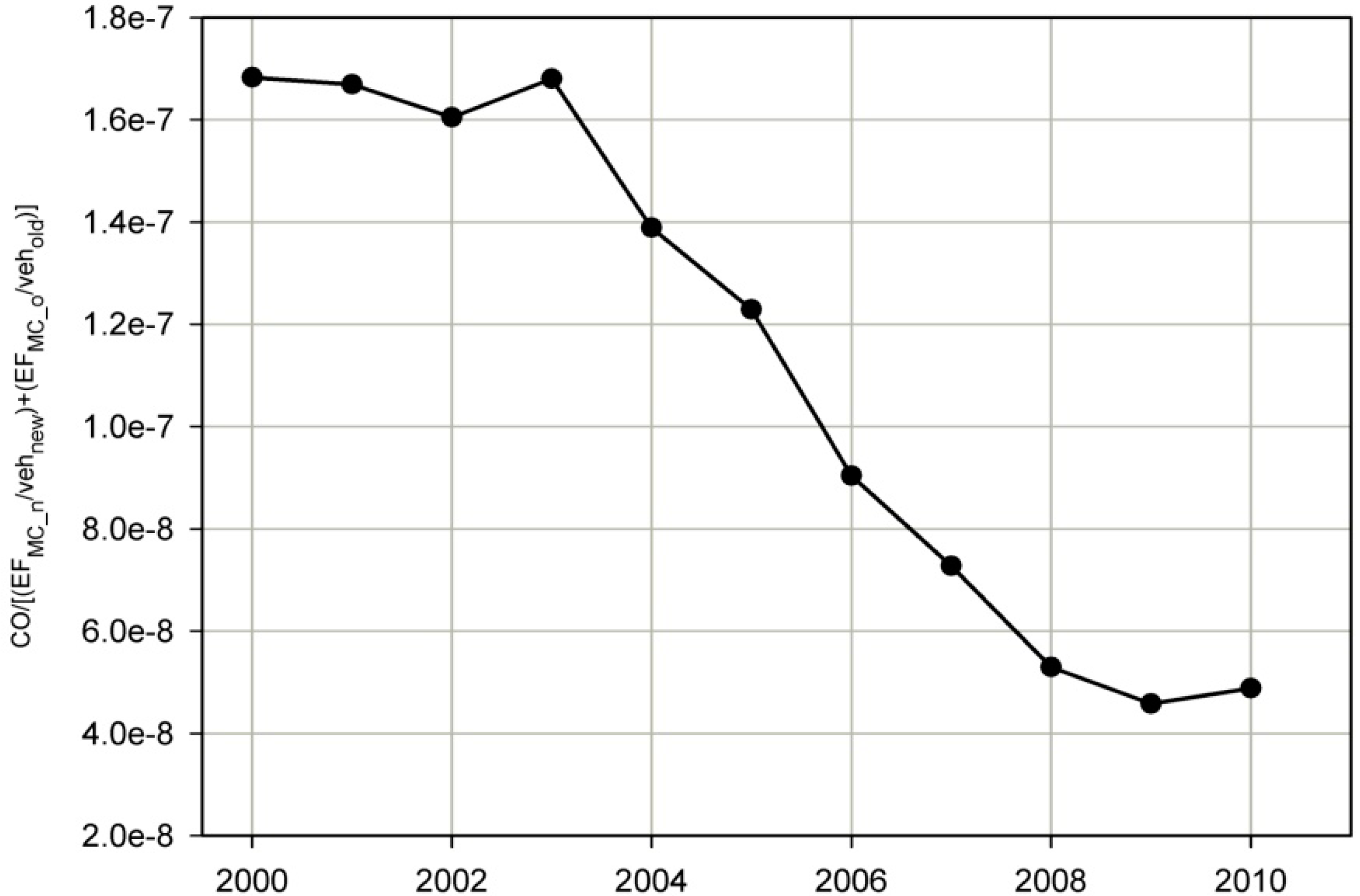
Figure 4). In
Figure 5, the annual mean of CO in the MCMA was normalized by the gross estimate of the total vehicle emissions using the above-mentioned emission factors. The flat trend in the first period indicates the effect of change in the vehicle composition; the decrease in CO was caused probably by the vehicle replacement. The decrease in the second period could be due to improved emission factor over the value used in the estimate, better traffic control, or decrease in the background concentration (which could have been occurring in the first period as well). However, it is not clear what the most important factor was.
Figure 4.
Distributions of vehicles by model year in the MCMA, GMA, and MMA from 2000 to 2010 based on data from
www.inegi.gob.mx (accessed on 15 February 2012).
Figure 4.
Distributions of vehicles by model year in the MCMA, GMA, and MMA from 2000 to 2010 based on data from
www.inegi.gob.mx (accessed on 15 February 2012).
Vehicle density is largest in the MCMA (
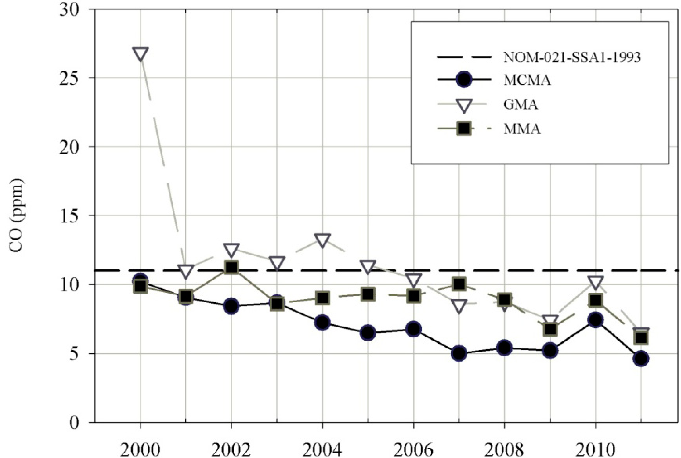
Figure 4), but vehicle emission regulations are stricter in the MCMA than in the GMA and MMA, which may have contributed to the satisfaction of the Mexican air quality standard for CO of 11 ppm (maximum value of 8-h moving averages) and a notable decrease in the annual trend in the MCMA over the analysis period.
In the GMA, the standard was exceeded in 2000, 2002, 2003, 2004, and 2005; the maximum CO concentrations were close to the limit in 2001, 2006, and 2010; and the standard was satisfied in the remaining years (
Figure 6). Assuming the emission factors mentioned above, in 2010, the effective emission factor weighted by the number of vehicles in each model-year category was 3.8 g/km in the MCMA, 5.0 g/km in the GMA, and 4.9 g/km in the MMA. The relatively high density of vehicles in the GMA (
Figure 4), together with the high estimated effective emission factor, may have led to the high CO concentrations in the GMA. Importantly, 7 of the 8 air-monitoring stations in the GMA are close (<200 m) to heavily trafficked roads. Thus, these stations may have preferentially detected CO from vehicular activity because CO emissions were poorly diluted near the stations. In contrast, the monitoring stations in the MCMA and MMA are mainly located close to moderately trafficked roads.
Figure 5.
Influence of the total vehicle emissions in the CO annual mean concentration in the MCMA. Total vehicle emissions was calculated as the sums of the products between emission factors (EFMC_n or EFMC_o) and the annual vehicle amount according to the model division: model ≥ 1994 (Vehnew) and model < 1994 (Vehold).
Figure 6.
Maximum values of 8-h moving-average CO concentrations in the three Mexican metropolitan areas. The dashed horizontal line indicates the MPL in Mexico.
Figure 6.
Maximum values of 8-h moving-average CO concentrations in the three Mexican metropolitan areas. The dashed horizontal line indicates the MPL in Mexico.
In the GMA, various factors seem to have influenced the annual trend (
Figure 3b). Vehicular emissions verification was established in 1991, but was suspended without clear reasons in 1992 [
19]. Until 2001, when the vehicular verification became mandatory, there was no system for penalty against violation. Upon the introduction of NOM-041-SEMARNAT-2006, the ratio of vehicles satisfying the CO emission regulation rose from 15% in 2005 to 30% in 2006, 36% in 2007, and 28% in 2008, although the ratio dropped to 18% in 2009 [
19]. To evaluate its effect, temporal trends in two periods (2003–2005 and 2006–2008) were examined by linear regression analysis, but no significant difference was found between the two periods. Therefore, there is no simple explanation for the temporal trend of CO in the GMA.
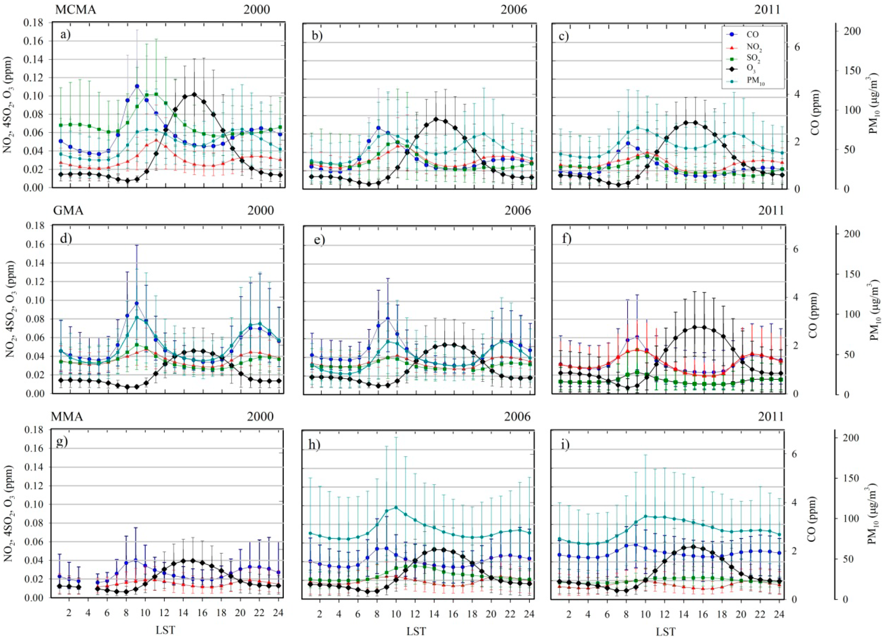
Figure 7 shows the hourly behavior of CO in the MCMA, GMA, and MMA in 2000, 2006, and 2011. In all study areas, the CO levels increased sharply at 08–09 local standard time (LST), coincident with the beginning of ordinary human activities. Around 18 LST, when the workday usually ended, the CO concentrations began to rise and eventually peaked at 21–22 LST (the evening rush hours in Mexican urban areas) at values lower than those in the morning. The difference between the shapes of the peaks can be explained as follows: in the morning, vehicle use was high for a short period of time because people were going to work and taking their children to school; in the afternoon, vehicle use was distributed over various times as students returned from their school activities; in the evening, vehicle use increased as people returned from work, but at a slower rate and at a lower intensity than in the morning. A more stable atmosphere in the morning than in the evening also contributed to the difference between the shapes of the peaks [
29].
Figure 7.
Diurnal behavior of CO, NO2, SO2, O3, and PM10 in the MCMA (a–c), GMA (d–f), and MMA (g–i) during 2000, 2006, and 2011. The bars indicate the range from the 10th to the 90th percentiles.
Figure 7.
Diurnal behavior of CO, NO2, SO2, O3, and PM10 in the MCMA (a–c), GMA (d–f), and MMA (g–i) during 2000, 2006, and 2011. The bars indicate the range from the 10th to the 90th percentiles.
In the MCMA, the morning peak shifted from 09 LST in 2000 and 2001 to 08 LST in subsequent years (
Figure 7a–c.). A probable cause for this shift is the rapid increase in the fleet density of newer-model vehicles (
Figure 4) from 2000 to 2005, which may have caused a progressive saturation of the roads and reduced the mean vehicle speed from 38.5 km/h in 1990, to 21 km/h in 2004, to 17 km/h in 2007 [
30], prompting people to shift their daily schedule to earlier hours.
3.2. Nitrogen Dioxide
Nitric oxide (NO) and nitrogen dioxide (NO
2) are collectively called nitrogen oxides (NOx). They play important roles in ozone formation and depletion as well as in secondary particle formation. According to INEM-2005 [
27], the main sources of NOx in Mexico in 2005 have been vehicles (44.7%), natural sources (38.6%), and industry (13.2%).
Figure 2b shows the seasonal variation of NO
2 in the three study areas. Minima occurred in summer (June to September), and maxima in winter, although there were considerable fluctuations.
The annual mean concentration of NO
2 in the MCMA remained nearly constant from 2003 to 2010, but fell 9% from 2010 to 2011 (
Figure 3d). In the MMA, the annual mean concentrations of NO
2 were considerably larger than the median values because of frequent episodes of high NO
2 concentrations (
Figure 3f).
In the GMA, the percentage of valid data was <75% from 2007 to 2010, so trends for the annual mean concentration of NO
2 could not be evaluated with a good accuracy for those years (
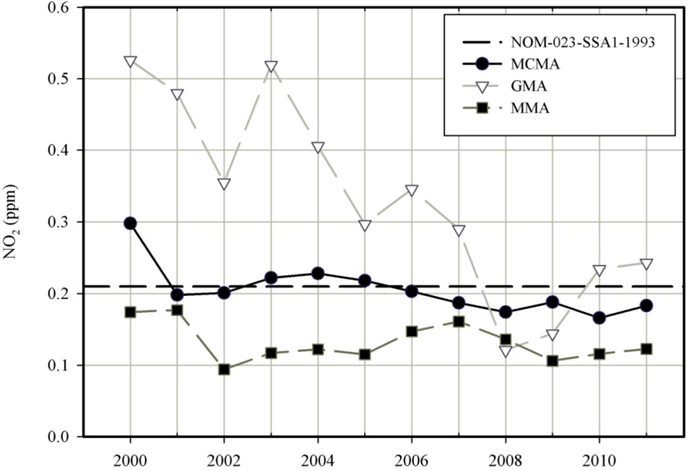
Figure 3e). Instead, we examined the annual trend for the maximum 1-h average, for which an environmental standard has been set (
Table 2,
Figure 8).
Figure 8 shows that the air quality standard was exceeded in all years from 2000 to 2011, except 2008 and 2009, and a decreasing trend is evident from 2000 to 2008.
Figure 8.
Maximum values of 1-h averages of NO2 concentrations in the three Mexican metropolitan areas. The dashed horizontal line indicates the maximum permissible limit (MPL) in Mexico.
Figure 8.
Maximum values of 1-h averages of NO2 concentrations in the three Mexican metropolitan areas. The dashed horizontal line indicates the maximum permissible limit (MPL) in Mexico.
The NO
2 concentrations in all study areas peaked in the morning and again in the evening, coincident with increased NO
2 emissions during the morning and evening rush hours (
Figure 7). In the MCMA, the morning peak occurred at 10–11 LST, whereas the evening peak occurred at 20–21 LST, almost at the same time as the evening CO peak. The ratio of the morning NO
2 peak height to the evening NO
2 peak height was much larger in the MCMA than in the GMA and MMA, possibly because more NO and VOCs, which oxidize NO to NO
2, were emitted in the morning than in the evening in the MCMA.
In the GMA, the morning NO2 concentration peaked at 10 LST from 2000 to 2006, but at 09 LST in 2010, almost 1 h earlier than in the MCMA. In 2011, the morning NO2 peak coincided with the morning CO peak. This behavior implies that the reaction between NO and oxidants such as VOCs and O3 was faster in the GMA than in the MCMA.
In the MMA, after 2004, the morning NO2 peaks at 09–10 LST were coincident with the morning CO peaks. However, in 2000 and 2001, the morning NO2 peaks were observed at 10–11 LST, almost 1 h later than the CO peaks.
3.3. Sulfur Dioxide
According to INEM-2005 [
27], the main source of SO
2 in Mexico in 2005 was industrial activity, accounting for 91.1% of total SO
2 emissions (2825 kton/year). Generation of electricity accounted for 49.7% of the industrial total (1403 kton/year), whereas extraction and processing of petroleum together with manufacturing of petrochemicals accounted for 39.8% of the industrial total (1124 kton/year).
In all study areas, high concentrations of SO
2 were recorded during the winter, whereas low concentrations were recorded during the rainy season, owing to dissolution of SO
2 in cloud water [
31] and removal by wet deposition (
Figure 2c).
In the GMA, maximum monthly SO
2 concentrations occurred from November to January, whereas minimum concentrations were recorded over a relatively wide range of months from June to October. In the MMA, behavior was irregular from 2000 to 2003 (concentration data for some months were not included in the source database and are therefore missing in
Figure 2c). From 2004 to 2009, concentration data for all months satisfied the 75% valid-data criterion, and the behavior was a little more regular, with maximum values in July (2004) and from December to February (2004–2009), and minimum values in July (2007, 2008), September (2004, 2006, 2009), and October (2005).
The annual mean concentration of SO
2 in the MCMA decreased ~67% from 2000 to 2011 (
Figure 3g). The annual mean values were substantially larger than the median values because of sporadic occurrences of particularly high values. The annual mean values for the GMA showed a generally increasing trend from 2000 to 2004, but a decrease of 68% from 2005 to 2011 (
Figure 3h). The annual mean values for the MMA showed a decrease of 36% from 2004 to 2011 (
Figure 3i).
The NOM-022-SSA1-2010 air quality standard for annual mean concentration of SO
2 was satisfied over the entire analysis period in all study areas (
Figure 3). The 24-h-average maximum permissible limit (MPL), however, was satisfied only in the GMA and MMA during the analysis period (
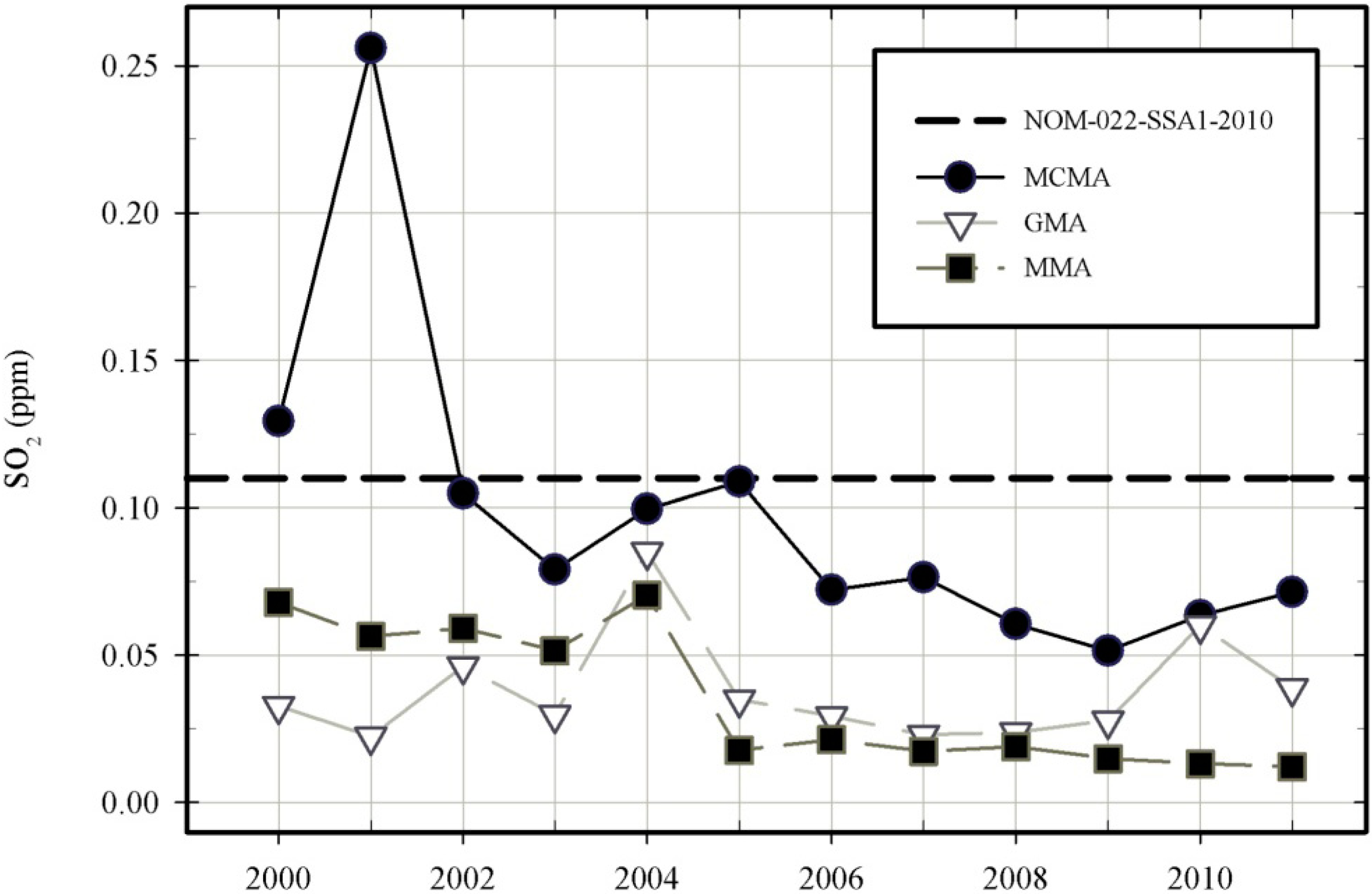
Figure 9). The MCMA exceeded the 24-h-average MPL of 0.11 ppm in 2000 and 2001 (0.129 ppm and 0.256 ppm, respectively), and matched or came close to the 24-h-average MPL in 2002 and 2005 (0.11 ppm and 0.109 ppm, respectively). The 24-h-average concentration of SO
2 in the GMA was below the MPL by a wide margin throughout the analysis period. MMA had the lowest 24-h-average maxima of all study areas from 2004 to 2010. Furthermore, three groups of concentration levels can be distinguished: a first group from 2000 to 2001, a second from 2002 to 2005, and a third from 2006 to 2011. The reduction of SO
2 concentration in the MCMA from 2001 to 2002 can be attributed to implementation of the PROAIRE Program to Improve Air Quality in the MCMA 2002–2010, which provided guidelines and action plans for reducing emissions from combustion of fossil fuels in industry and power generation. In addition, in 2004, the Mexican National Refining System started distributing Premium gasoline (containing 250–300 ppm sulfur) to replace Magna gasoline (containing 300–500 ppm sulfur). The concentration of SO
2 in the MCMA decreased from 2005 to 2006, and the SO
2 levels in all study areas decreased significantly in 2006 (
Figure 3), when NOM-086-SEMARNAT-SENER-SCFI-2005, which limited the sulfur concentration in liquid and gaseous fossil fuels sold in the MCMA, GMA, and MMA, was put into effect. In October 2006, refiners reduced the concentration of sulfur in both Premium and Magna gasoline to 30–80 ppm, and the maximum allowable sulfur in diesel oil has been reduced from 500 ppm to 15 ppm since January 2009 [
32,
33]. Moreover, November 2007 was the deadline to fulfill the NOM-148-SEMARNAT-2006 was implemented, which strengthened the requirements for the recovery of sulfur in oil-refining processes to reduce the amount of sulfur in emissions by 90% or more.
Figure 9.
Maximum values of 24-h averages of SO2 concentrations in the three Mexican metropolitan areas. The dashed horizontal line indicates the MPL in Mexico.
Figure 9.
Maximum values of 24-h averages of SO2 concentrations in the three Mexican metropolitan areas. The dashed horizontal line indicates the MPL in Mexico.
Table 3.
Estimated annual emission of SO2 (tons/year) from the Tula complex.
Table 3.
Estimated annual emission of SO2 (tons/year) from the Tula complex.
| Year | Power Plant | Oil Refinery |
|---|
| 2002 | 158,330 1 | n/e |
| 2005 | 132,374 2 | 132,368 2 |
| 2007 | n/e | 75,057 *,3 |
| 2008 | 135,705 4 | 76,400 4 |
| 2009 | n/e | 61,857 *,3 |
| 2010 | 135,705 5 | n/e |
Stationary sources of SO
2 substantially influenced the SO
2 levels in the MCMA. The Tula industrial complex, ~60 km northwest of the center of Mexico City, has two major stationary sources of SO
2: a power plant and an oil refinery. Rivera
et al. [
9] estimated that the Tula industrial complex emitted 384 ± 103 tons of SO
2 per day, and, using model simulations, de Foy
et al. [
8] estimated that the long-term-average contribution of SO
2 from the Tula complex to the MCMA airshed was 20%.
Table 3 lists estimated annual emissions of SO
2 from the Tula complex for 2002, 2005, and 2007–2010. The large reduction in SO
2 emission from the refinery (around 42% from 2005 to 2008) was likely due to the implementation of NOM-148-SEMARNAT-2006. More details about it could be found in Alcantara-Gonzalez and Cruz-Gomez [
33].
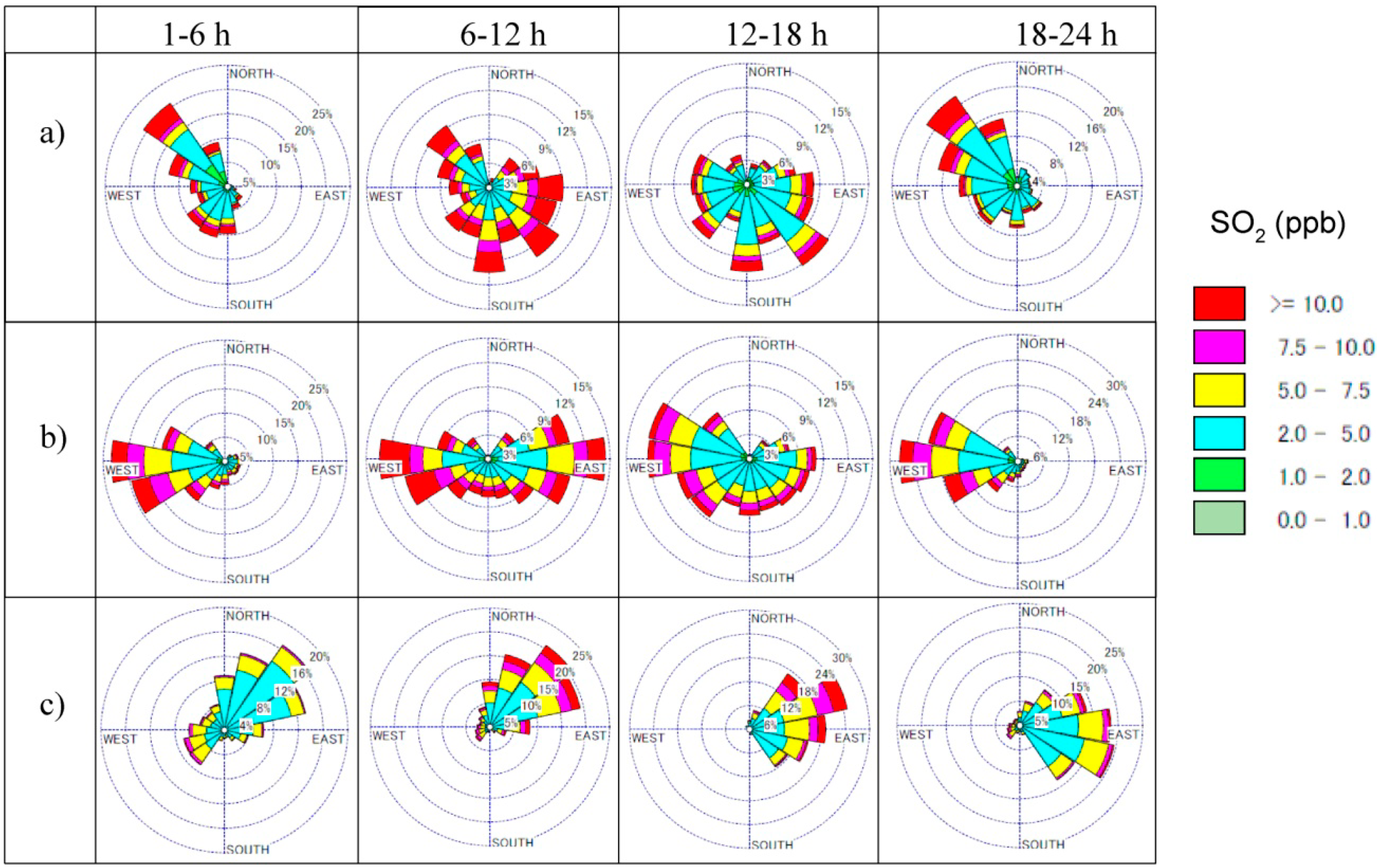
Figure 10.
Six-hour-interval frequency distributions of SO2 concentrations and direction recorded at meteorological observatories from 2006 to 2011 in the (a) MCMA, (b) GMA, and (c) MMA.
Figure 10.
Six-hour-interval frequency distributions of SO2 concentrations and direction recorded at meteorological observatories from 2006 to 2011 in the (a) MCMA, (b) GMA, and (c) MMA.
Hours are referred as LST.
The levels of SO
2 in the MCMA and MMA were affected by wind speed and direction.
Figure 10 shows 6-h-interval frequency distributions of wind speed and direction recorded at meteorological stations from 2006 to 2011 in the MCMA, GMA, and MMA and SO
2 hourly average concentrations recorded by air monitoring stations in each area. Due to the location of the Tula complex, the level of SO
2 in the MCMA was particularly influenced by north-to-northwest winds. High frequency of high SO
2 under northwest wind condition is observed in the 1–6 h and 18–24 h intervals (
Figure 10). In the 6–12 h interval, the behavior is different with high frequency of high SO
2 occurring in most wind directions. The high SO
2 in the 6–12 h interval is probably due to the road traffic. The diurnal behavior of SO
2 in the MCMA, GMA, and MMA during 2000, 2006, and 2011 is shown in
Figure 7. Similar to the behavior of CO and NO
2, maximum SO
2 concentrations in the MCMA occurred at 10–11 LST in 2000 and 2001, but at 09–10 LST in subsequent years. In the GMA, the maximum morning SO
2 concentration occurred at 09 LST, coincident with the CO maximum (
Figure 7d–f). At night, broad peaks occurred around 22 LST, 1 h later than the CO and NO
2 maxima. The morning and evening SO
2 peaks suggest a relationship between SO
2 levels and vehicle activity. However, it is important to note that 7 of the 8 air-monitoring stations in the GMA are close to heavily trafficked roads and may have preferentially detected SO
2 from vehicle activity.
The diurnal behavior of SO
2 in the MMA was different from that of CO and NO
2 (
Figure 7g–i). The highest SO
2 concentrations were recorded in the morning at 11–12 LST from 2004 to 2008. After 2009, the SO
2 concentration peaked between 11 and 13 LST, quite different from the behavior of CO and NO
2, which peaked at 08 and 09 LST. These differences were related to wind direction (
Figure 10c); when the wind came from the northeast, the SO
2 concentrations tended to rise. This fact suggests that some of the SO
2 in the MMA originated from sources in the northeast part of the MMA or outside of Mexico.
3.4. Ozone
Figure 2d shows the seasonal trends for O
3. O
3 concentrations rise in winter, reaching maximum values in spring, when weather conditions help promote photochemical production of O
3. Ozone is produced by photolysis of NO
2 but is consumed during oxidation of NO in complex reaction chains involving VOCs and hydroxide radicals. The concentration of O
3 was low in summer and fall, when rainy and cloudy conditions reduced solar radiation, suppressing photolysis of NO
2 to produce O
3.
The annual mean O
3 concentration in the MCMA decreased rapidly by around 25% from 2000 to 2004, but from 2005 to 2010, the rate of decrease became more gradual, around 13% (
Figure 3j). In the GMA, the annual mean O
3 concentration increased sharply, around 47%, from 2000 (0.022 ppm) to 2011 (0.034 ppm) (
Figure 3k). In the MMA, the O
3 concentration increased significantly (~42% increase in annual mean) from 2000 (0.020 ppm) to 2011 (0.028 ppm) (
Figure 3l).
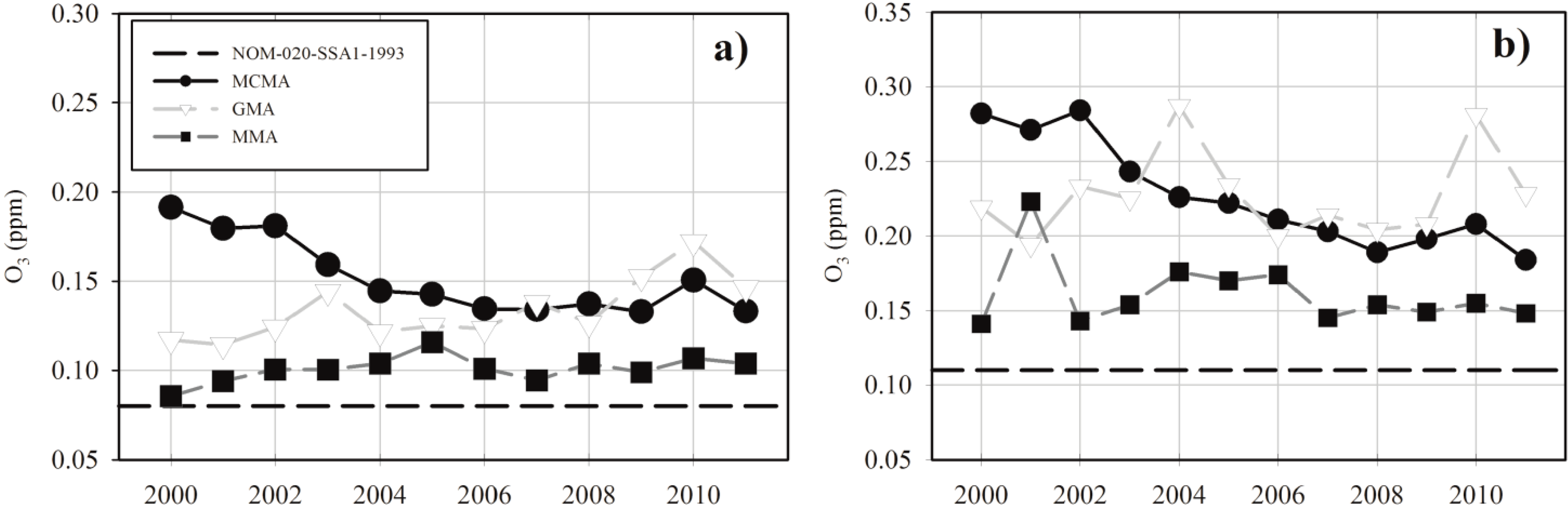
Over the analysis period, none of the study areas satisfied the NOM-020-SSA1-1993 air quality standard [MPL: 0.11 ppm (1-h average), 0.08 ppm (fifth maximum of 8-h moving averages)]. The O
3 concentration in the MCMA fell considerably over the analysis period, but was still well above the MPL, exhibiting the highest fifth maxima in 8-h moving averages among the study areas until 2008 (
Figure 11a).
The O
3 concentration in the GMA exceeded the MPLs over the analysis period (
Figure 11). As with the 98th percentile values of daily averages (
Figure 3), the fifth maxima of 8-h moving averages showed an increasing trend (
Figure 11a). However, the maximum values of 1-h averages showed considerable fluctuations, implying that the potential to generate high-concentration O
3 was retained and that severe photochemical smog could occur under favorable conditions.
Figure 7 shows the diurnal behavior of O
3 in the MCMA, GMA and MMA. A local minimum occurred in the early morning because depletion of O
3 was enhanced as the concentration of NO increased (primarily NO emitted from vehicles during rush hours). Later, the increased concentration of NO
2, increased emission of VOCs, and intensified solar radiation led to a net increase of O
3, and the daily maximum occurred in the early afternoon. Toward evening, the O
3 concentration decreased because photochemical production of O
3 became less frequent than destruction of O
3 on solid surfaces and reaction of O
3 with NO. In the MCMA, maxima occurred at 15 LST in 2000 and 2001, but at 14 LST in subsequent years, a shift similar to that for CO, NO
2, and SO
2 and probably associated with the shift of human activity to earlier hours. In the GMA, the O
3 concentration peaked at 15 LST (
Figure 7d–f), 1 h later than in the MCMA (14 LST), and reached minima at 08 LST. In the MMA, the O
3 concentration peaked at 14–15 LST, and the minima occurred at 08 LST over the entire study period. The daily maximum average of O
3 concentration in the MCMA was 46% and 69% higher than in the GMA and MMA, respectively.
Figure 11.
(a) Annual fifth maximum values of 8-h moving averages and (b) maximum values of 1-h averages of O3 concentrations in the three Mexican metropolitan areas. The dashed lines indicate the MPL in Mexico.
Figure 11.
(a) Annual fifth maximum values of 8-h moving averages and (b) maximum values of 1-h averages of O3 concentrations in the three Mexican metropolitan areas. The dashed lines indicate the MPL in Mexico.
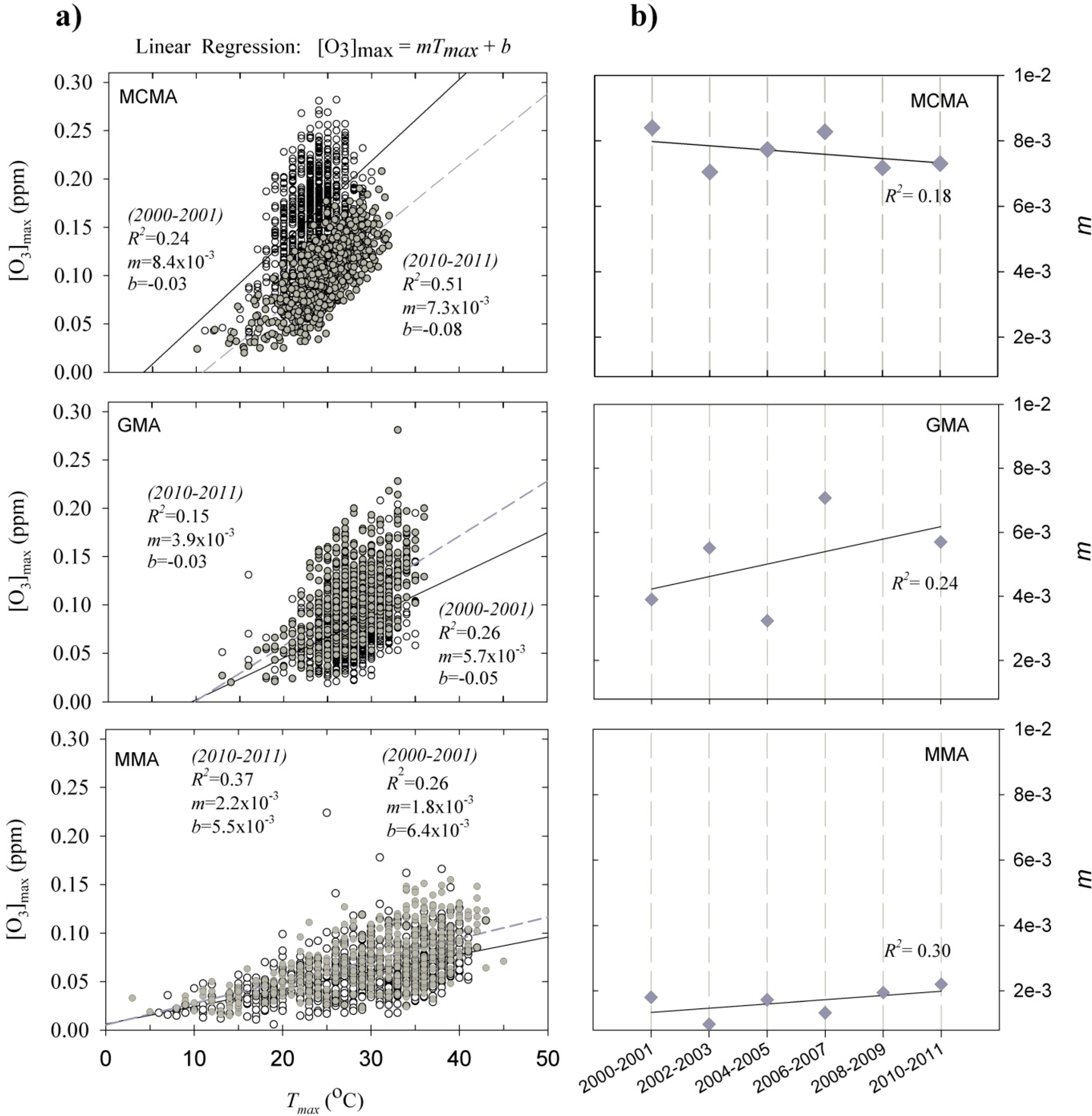
Production of O
3 depends on the amount and composition of precursor substances and on the intensity of solar radiation. To separate the two factors, we examined the correlation between the daily maximum O
3 concentration ([O
3]
max) and the daily maximum temperature (T
max), a proxy for the radiation intensity.
Figure 12a shows scatter plots for the periods 2000–2001 and 2010–2011 and the variation of the linear regression slopes during different periods of time. Generally, [O
3]
max increases with T
max because the rate of photochemical reaction is higher at higher temperature. Within each region, differences in the slopes and y intercepts of the linear regression lines indicate differences in O
3 production efficiency due to factors other than temperature.
Figure 12 shows that, from 2000–2001 to 2010–2011, the slopes of the lines decreased in the MCMA but increased in the GMA and MMA. Moreover, the range of T
max changed little from 2000–2001 to 2010–2011. To examine if the temporal change in the slope of the regression line was significant, regression analysis was repeated for other two-year periods 2002–2003, 2004–2005, 2006–2007, and 2008–2009.
Figure 12b shows the result. Although the fluctuation is large, decreasing trend in the MCMA and increasing trend in the GMA and MMA could be confirmed. Therefore, additional factors other than temperature (such as solar radiation and difference in the VOC concentration, which is not included in the regular air-monitoring data), may be involved in the annual trend of O
3 concentration.
3.5. Particulate Matter (PM10)
According to INEM-2005 [
27], the main sources of PM
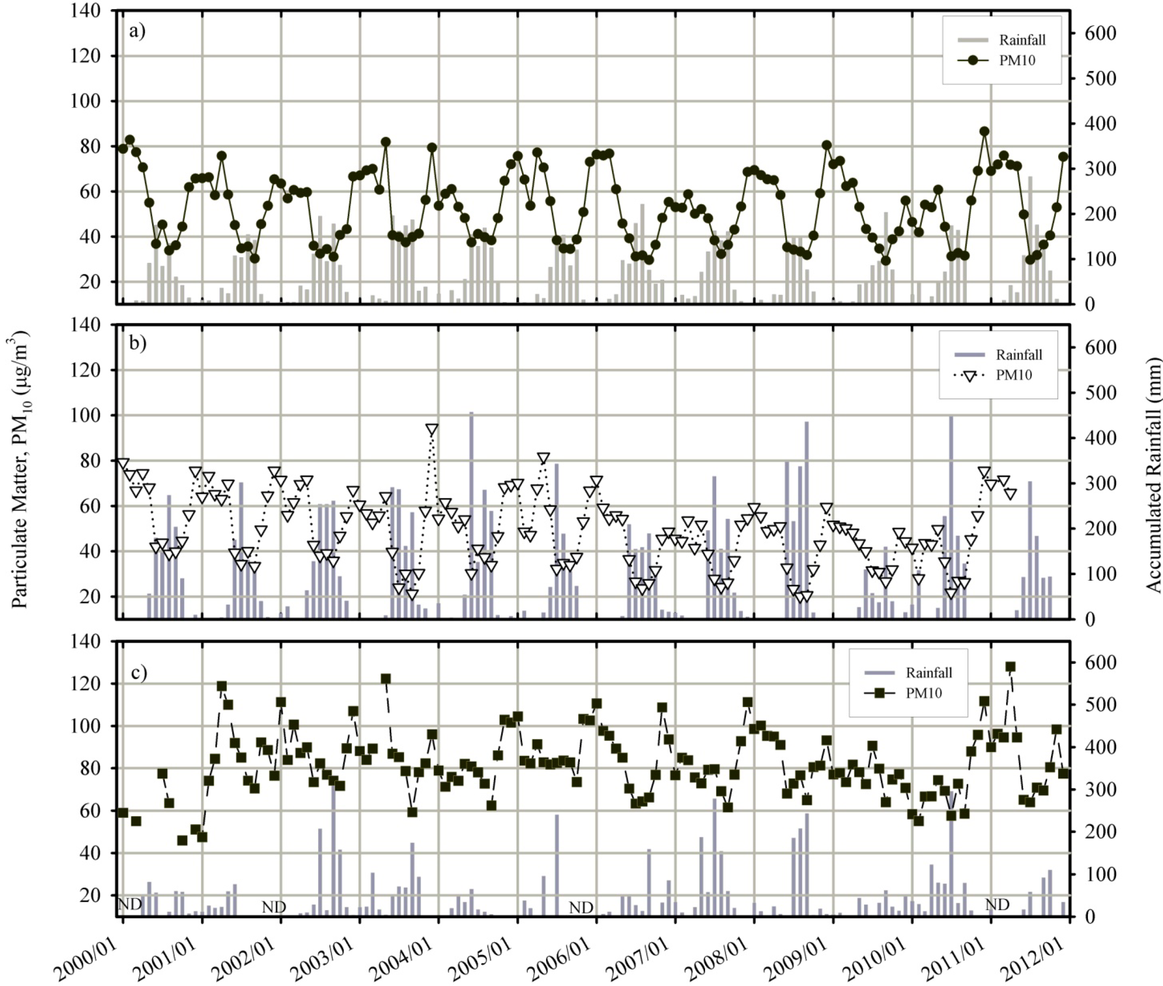
10 in Mexico are area sources (industrial, commercial, agricultural, household combustion). In all three study areas, the highest monthly rainfall occurred in the same month as the minimum PM
10 concentration, mostly in summer (
Figure 13). PM
10 concentrations started to rise in fall and peaked in winter. Exceptionally low PM
10 concentrations were recorded from August to November 2006 and from May to October 2007 in the MCMA and GMA, when several tropical cyclones in the northeastern Pacific affected these areas. PM
10 concentrations in the MMA apparently were influenced only weakly by rainfall; however, the data for accumulated rainfall could be misleading due to long periods of missing rainfall data. Besides, higher PM
10 concentrations in the MMA from July 2010 to April 2011 occurred due to the increase of construction activities and resuspension of soils, among others, as consequences of the rebuilding of the area after the severe flooding caused by the hurricane Alex.
Figure 12.
(a) Correlations between daily maximum temperature and daily maximum O3 concentration in the MCMA, GMA, and MMA for the periods 2000–2001 and 2010–2011 (white and gray circles indicate values for the periods 2000–2001 and 2010–2011, respectively; the black and dashed gray lines are linear regression lines for the periods 2000–2001 and 2010–2011, respectively) and (b) variation of the linear regression slopes (m) during different periods of time in the MCMA, GMA and MMA.
The annual mean concentration of PM
10 in the MCMA over the study period was close to the NOM-025-SSA1-1993 air quality standard (50 µg/m
3) and did not show any clear long-term trend (
Figure 3m). In the GMA, the annual mean concentration of PM
10 decreased by 27.5% from 2000 to 2010 (
Figure 3n), and the air quality standard has been satisfied in the GMA since 2006. In the MMA, the annual mean concentration of PM
10 was higher than 50 µg/m
3 and 37% higher than that in the MCMA and around 42% higher than that in the GMA from 2001 to 2009; and the 98th percentile values of daily averages exceeded the limit of 120 µg/m
3 (
Figure 3o). The geographic conditions of MMA create long periods of severe drought, which together with anthropogenic activities enhance emission of particulate matter.
Figure 13.
Temporal variation of monthly averages of PM10 concentration and accumulated monthly rainfall in the (a) MCMA, (b) GMA, and (c) MMA.
Figure 13.
Temporal variation of monthly averages of PM10 concentration and accumulated monthly rainfall in the (a) MCMA, (b) GMA, and (c) MMA.
ND: rainfall data not available.
The diurnal variations of PM
10 in the study areas exhibited two peaks, a consequence of daily activities typical of Mexican urban areas (
Figure 7). In the MCMA, the PM
10 concentration began rising at 05–06 LST, coincident with the beginning of anthropogenic activities. The PM
10 concentration peaked at 10 LST in 2000 and 2001, but at 09 LST in subsequent years (1 h later than the CO peak). After the morning peak, a decrease in PM
10 concentration was recorded followed by an evening peak at 19 LST. The PM
10 evening peak appeared 2 or 3 h earlier than the CO evening peak, owing to differences between the CO and PM
10 source characteristics, especially in the afternoon, when secondary aerosol produced in photochemical reactions [
34,
35] and wind-blown dust from dry areas [
35,
36] contributed to PM
10.
In the GMA, the morning PM10 peak occurred at 09 LST, coincident with the maximum CO and SO2 concentrations and 1 h earlier than the maximum NO2 concentration. In the evening, the PM10 concentration peaked at 21 LST, coincident with the maximum CO and NO2 concentrations and 1 h earlier than the SO2 maximum concentration.
The PM
10 concentration in the MMA began rising early in the morning (around 05–06 LST), coincident with the beginning of anthropogenic activities, and peaked at around 10 LST. The decay from the morning peak was more gradual than that in the other metropolitan areas owing to high-level emissions of primary particles from resuspension of road dust in the daytime from unpaved and paved roads (which represents about 44% of the total PM
10 emission in the MMA) and activities related to construction and other industries (
Table 4). Therefore, road dust in the MMA is one of the important factors for the relatively high PM10 in the daytime even outside rush hours. Among the study areas, the annual estimated emission of PM
10 from major sources was highest in the MMA (
Table 4).
Table 4.
Estimated annual emission of PM10 (tons/year) from major sources in the three Mexican metropolitan areas.
Table 4.
Estimated annual emission of PM10 (tons/year) from major sources in the three Mexican metropolitan areas.
| Source | MCMA 1 | GMA 2 | MMA 3 |
|---|
| Construction activities | 845 | 2983 | 14,871 |
| Paved roads | 6428 | n/e | 11,320 |
| Unpaved roads | 10,618 | n/e | 16,459 |
| Food industry | 821 | 7835 | 486 |
| Mobile | 3720 | 743 | 2090 |
| Industrial emissions (except food industry) | 4900 | 1236 | 8061 |
| Area (except for construction activities) | 3763 | 6,004 | 140 |
| Natural (including soil erosion) | 511 | n/e | 10,195 |
| Total emission in the area | 31,606 | 18,801 | 63,622 |


