Article

Tracing Sources of Total Gaseous Mercury to Yongheung Island off the Coast of Korea

1
Department of Environmental Science, Kangwon National University, 192-1, Hyoja-2-dong, Chuncheon, 200-701 Gangwon-do, Korea
2
Department of Civil and Environmental Engineering, Clarkson University, Potsdam, NY 13699, USA
3
Department of Environmental & Energy Engineering, Anyang University, 22 Samdeok-ro, Manan-gu, Anyang, 430-714 Gyeonggi-do, Korea
*
Author to whom correspondence should be addressed.
Atmosphere 2014, 5(2), 273-291; https://doi.org/10.3390/atmos5020273
Submission received: 27 February 2014 / Revised: 11 April 2014 / Accepted: 15 April 2014 / Published: 30 April 2014
(This article belongs to the Special Issue Atmospheric Mercury)

Abstract

:
In this study, total gaseous mercury (TGM) concentrations were measured on Yongheung Island off the coast of Korea between mainland Korea and Eastern China in 2013. The purpose of this study was to qualitatively evaluate the impact of local mainland Korean sources and regional Chinese sources on local TGM concentrations using multiple tools including the relationship with other pollutants, meteorological data, conditional probability function, backward trajectories, and potential source contribution function (PSCF) receptor modeling. Among the five sampling campaigns, two sampling periods were affected by both mainland Korean and regional sources, one was caused by mainland vehicle emissions, another one was significantly impacted by regional sources, and, in the remaining period, Hg volatilization from oceans was determined to be a significant source and responsible for the increase in TGM concentration. PSCF identified potential source areas located in metropolitan areas, western coal-fired power plant locations, and the southeastern industrial area of Korea as well as the Liaoning province, the largest Hg emitting province in China. In general, TGM concentrations generally showed morning peaks (07:00~12:00) and was significantly correlated with solar radiation during all sampling periods.

1. Introduction

Mercury (Hg) is a toxic heavy metal of concern throughout the Northern Hemisphere. It is emitted from both anthropogenic and natural sources into the atmosphere mostly as inorganic forms. Atmospheric Hg does not generally constitute a direct public health risk at the level of exposure usually found [1]. However, once Hg is deposited into aquatic systems, it can be transformed into methylmercury (MeHg) which is very toxic and readily bioaccumulates through the food web and can affect the health of humans and wildlife. For MeHg in aquatic systems, it has been suggested that atmospheric deposition of inorganic Hg is an important source in many previous studies [2,3,4,5]; therefore, there is a need for research on the behavior of atmospheric Hg.
Anthropogenic sources of atmospheric Hg include combustion of coal and other fuels, mining activities, non-metal smelters, and waste incinerators, which emit 1960 ton/yr globally [6]. Atmospheric mercury exists mainly in three operationally defined inorganic forms: gaseous elemental mercury (GEM, Hg0), gaseous oxidized mercury (GOM, Hg2+), and particulate bound mercury (PBM, Hg(p)). GOM is highly soluble in water and readily deposits to surfaces. Thus, it has short residence time of 1–2 days [1,7]. The residence time of PBM is dependent on the size of particles, but, generally, it has been assumed to be a few days [8,9]. The predominant form of Hg in ambient air is GEM due to its low solubility in water, small deposition velocity, and relatively low reaction rates; therefore, it can be transported long distances and is often considered as a global transboundary pollutant (residence time = 0.5–1 yr) [7,10].
The region of largest anthropogenic Hg emissions is East and Southeast Asia, contributing 39.7% (396–1690 ton) of the total anthropogenic emissions according to an estimation in 2008 [6]. China accounts for three-quarters of these emissions, or about one third of the global total [6]. In addition, Hg emissions in China have dramatically increased since 1990, primarily because coal burning for power generation and for industrial purposes continues to increase while Hg emissions from Europe and North American have decreased. There are several studies predicting the contribution of Asian sources to Hg levels on other continents. Signeur et al. [11] estimated that the contribution of Asian anthropogenic emissions to the total Hg deposition over the continental United States ranged from 5% to 36% using a CTM (Chemical Transport Model). In addition, Jaffe et al. [12] observed a significant increase in Hg concentrations with prevailing westerly winds from continental Asia. Obrist [13] also measured enhanced mercury concentrations in the Colorado Rocky Mountains in the United States due to long-range transport from Asia with westerly winds.
In Korea, the history of atmospheric mercury measurements is relatively shorter than in the USA and Canada. Total gaseous mercury (TGM) was first measured by Kim and Kim [14] starting in the late 1980s in Seoul, Korea. They reported high concentrations of 14.4 ± 9.8 ng∙m−3. Recent studies showed much lower TGM concentrations ranging from 2.1 ng∙m−3 to 3.9 ng∙m−3 [15,16,17,18,19] due to the wider use of air pollution controls and more stringent regulations. Although Hg emissions in Korea have generally decreased since 1990, Hg levels in Korea may be still seriously affected by Chinese emissions because Korea is situated just west of China, the biggest Hg emitter in the world. This study was designed to identify the contribution of both Chinese emissions and local emissions on atmospheric Hg concentrations in Korea. The sampling site was the most western island in Korea, located in between eastern China and Korea, so that, depending on wind patterns, the effect of Chinese and local Hg emissions could be evaluated.

2. Results and Discussion

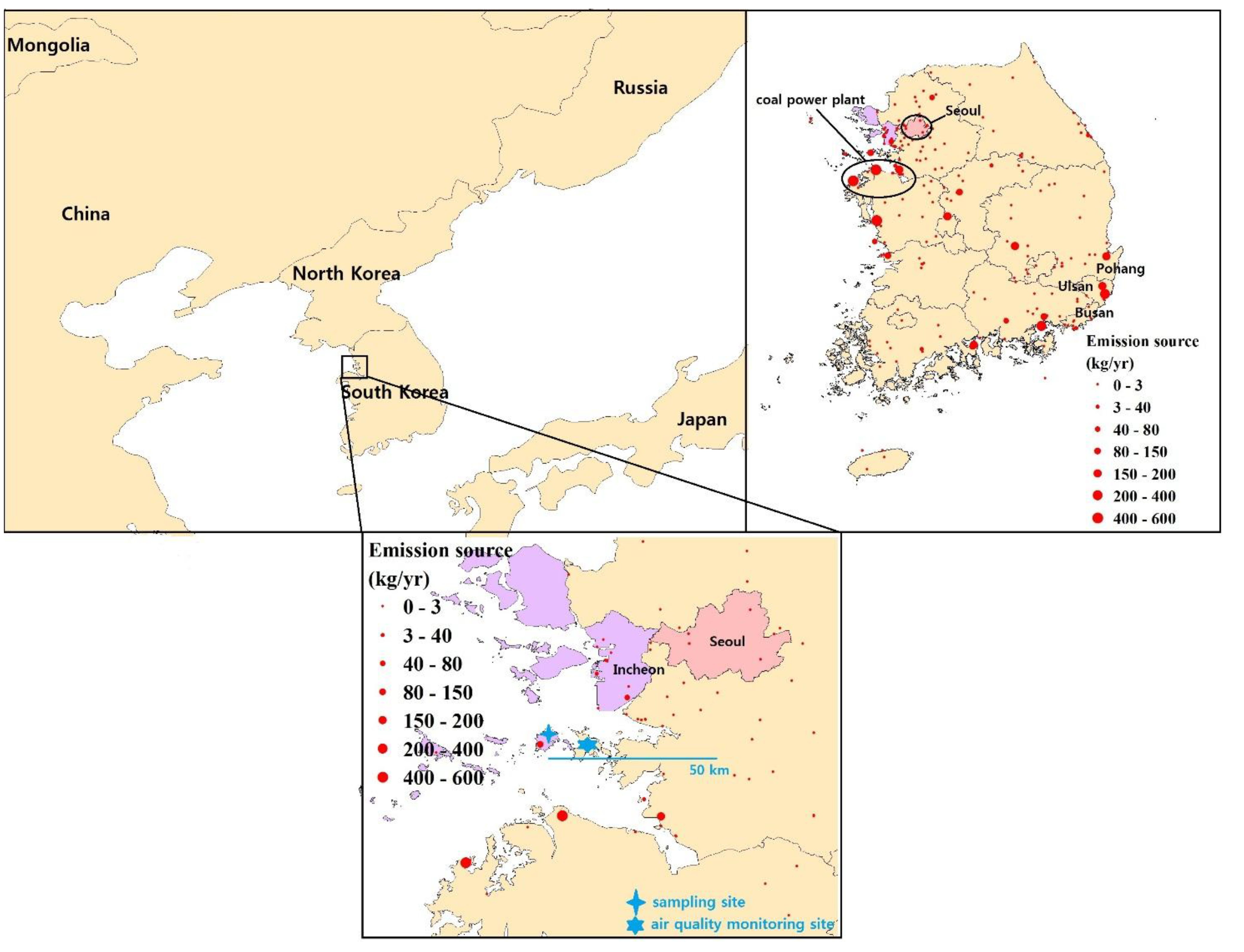
2.1. Sampling Description

The biggest local Hg source on Yongheung Island (Figure 1) is the Yongheung coal power plant (YCPP) (0.11 ton Hg∙yr−1 [20]) located approximately 4.5 km southwest of the sampling site. To the east of the sampling site, there are multiple mainland Hg sources in the industrial area of Incheon including the steel industry (1–57 kg∙yr−1) and waste incinerator (0–3 kg∙yr−1) (Figure 1). In addition, the Hg concentrations at this site can be impacted by Chinese emissions through long-range transport when there are prevailing westerly winds. There are also other local sources in western and northern areas (waste incinerator) and southern areas (coal-fired power plant) within 50 km of the sampling site. The total TGM emissions rate from all anthropogenic Hg sources in Korea is 32.2 ton∙yr−1 in 2005 [21].

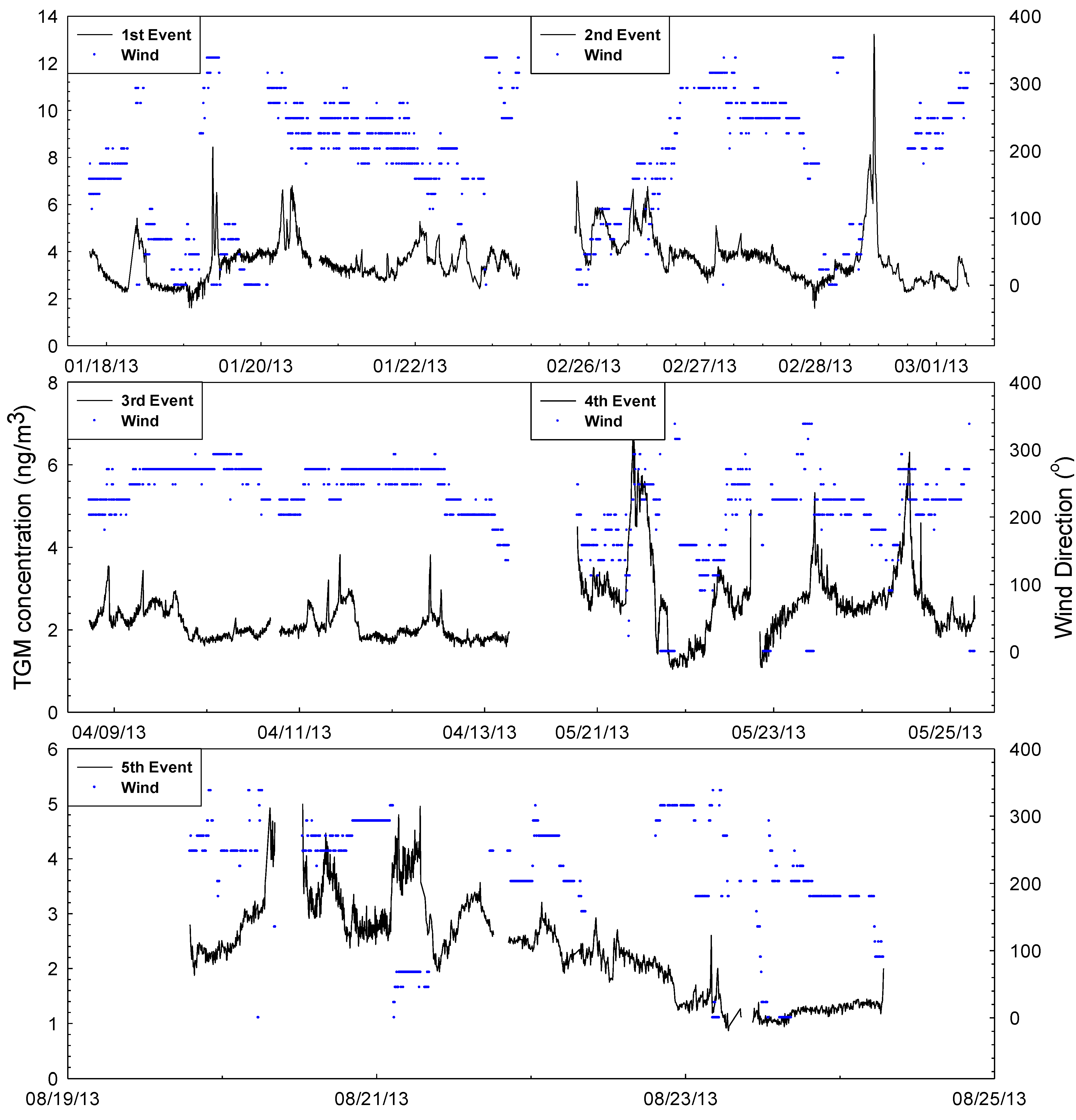
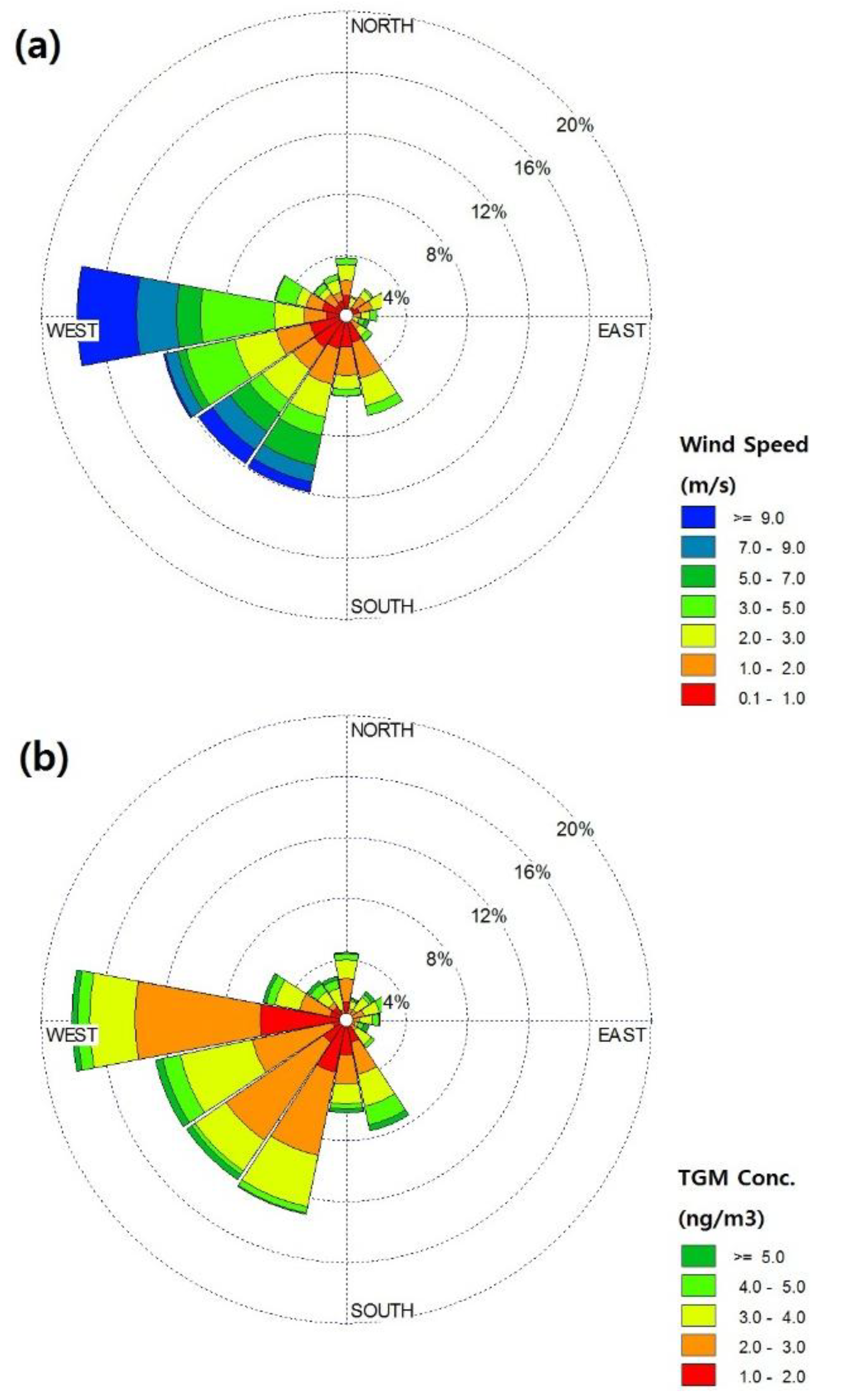
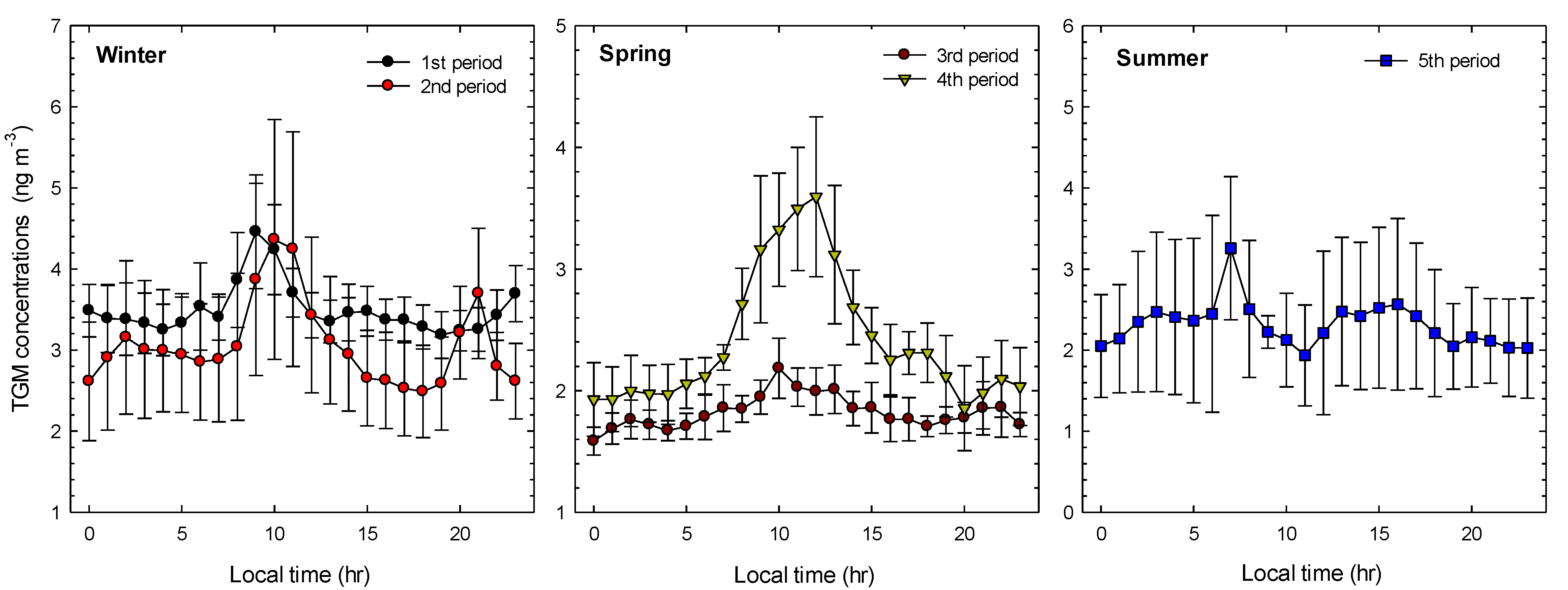
2.2. General TGM Patterns

The average TGM concentration was 2.87 ± 1.07 ng∙m−3 during the sampling periods (Figure 2). The seasonal TGM concentration was the highest in winter (January, February) (3.60 ± 0.97 ng∙m3), followed by in spring (April, May) (2.43 ± 0.83 ng∙m−3) and in summer (August) (2.29 ± 0.85 ng∙m−3) (Tukey HSD test, p-value < 0.001) (Table 1, Figure 2). Higher TGM concentrations in winter are generally observed in the Northern Hemisphere at least in part due to increased emissions and by the distinctive meteorological conditions including reduced mixing layer heights [22,23]. On the other hand, generally reduced TGM concentrations were seen during summer.
Table 1. Summarized seasonal total gaseous mercury (TGM) concentrations for five sampling periods.
SamplingDateSeasonTGM (ng∙m−3)Wind Speed (m∙s−1)Temperature (°C)Solar Radiation (W m−2)
1st Period2013.01.17–2013.01.21Winter3.49 ± 0.811.45 ± 1.051.00 ± 2.7168.94 ± 136.49
2nd Period2013.02.25–2013.03.013.67 ± 0.911.55 ± 1.412.59 ± 2.3340.55 ± 81.21
3rd Period2013.04.08–2013.04.13Spring2.09 ± 0.406.98 ± 2.565.58 ± 1.01238.99 ± 324.75
4th Period2013.05.20–2013.05.252.80 ± 1.001.56 ± 1.0813.60 ± 2.93252.30 ± 318.84
5th Period2013.08.19–2013.08.24Summer2.29 ± 0.851.03 ± 1.1525.74 ± 1.91180.55 ±274.40
These concentrations were considerably lower than those measured at urban sites in China and Taiwan, but in a similar range as urban sites in Korea and higher than in suburban and background areas of USA and Canada (Table 2). Considering that background TGM concentrations in locations not impacted by local emission source are typically 1.4–2.0 ng∙m−3 [24], TGM concentrations measured at this study were indeed affected by local and regional anthropogenic sources.
Figure 1. The Hg sampling site (with a cross mark) in this study and the national air quality monitoring site (with a star mark) for other atmospheric pollutants. The upper right panel indicates the anthropogenic TGM emission sources in Korea.
Atmosphere 05 00273 g001
During the sampling period, westerly and southwesterly winds were predominant (Figure 3); however, high TGM concentrations were associated with all wind directions (Figure 3). Low TGM concentrations (<2 ng∙m−3) were not observed with easterly winds, but the frequency of easterly winds was too low to indicate that mainland Korean sources were more important than southwesterly located YCPP or regional Chinese sources. The relative importance of local and regional sources will be discussed in more detail in the next section.
Diel variations in TGM concentration generally showed morning peaks (07:00–12:00) during all sampling periods (Figure 4). In urban areas, TGM concentrations are typically higher during the nighttime than during the daytime [25,26] due to a combination of GEM loss by daytime oxidation, increased use of household heating systems and decreased mixing height at night. In this study, higher nighttime TGM concentrations were not found in any sampling period (Figure 4). The sampling site is located in a remote island having a population of only 5815; therefore, Hg emissions from nighttime household heating systems were presumed to be not significant. Although the biggest anthropogenic source on this island (YCPP) operates continuously all year round, actual electricity usage generally fluctuates with a larger rate during the daytime than in the night (Korea Electric Power Generation, http://cyber.kepco.co.kr), which also might contribute to the higher daytime TGM concentration measured in this study.
Figure 2. Measured TGM concentrations (left y-axis) with wind direction (right y-axis) for five sampling periods.
Atmosphere 05 00273 g002
Some previous studies in rural and remote areas found that a maximum TGM concentration in mid-morning and a minimum at night was due to Hg emissions from natural surfaces including oceans and soils during times of increased solar radiation [27,28,29]. There are many studies showing that emissions of GEM from water and soil surfaces increase with increasing solar radiation [30,31,32]. Since the sampling site is located next to the beach, the emissions of Hg from the ocean surface could possibly elevate atmospheric TGM concentrations. Solar radiation was positively correlated with TGM concentration for all sampling periods (Table 3), suggesting the possibility of measurable volatilization from natural sources. TGM was also negatively correlated with wind speed and atmospheric temperature, and positively correlated with relative humidity for the whole sampling period although the relationship was not consistent for every individual sampling period (Table 3).
Table 2. Comparison of TGM concentrations with other studies.
CountrySiteYearRemarksTGM (ng∙m−3)Reference
KoreaSeoul2005–2006Urban3.4 ± 2.133
Seoul2005–2006Urban3.2 ± 2.123
Jeju*2006–2007Island3.9 ± 1.718
Chuncheon2006–2009Rural2.1 ± 1.525
This study2013Island2.9 ± 1.1
ChinaPearl River2008Background2.934
Guiyang2009Urban9.7 ± 10.235
Beijing1998Urban7.9 ± 34.936
TaiwanCentral Taiwan2010–2011Urban6.1 ± 3.737
U.S.A.Reno, Nevada2007–2009Suburban2.0 ± 0.738
Great Smoky Mt.2007Background1.6522
Detroit2002Urban3.139
CanadaNova Scotia2010–2011Rural1.4 ± 0.224
Figure 3. Wind rose (a) and pollution rose (b) for the entire sampling period.
Atmosphere 05 00273 g003
Table 3. Correlation coefficients of TGM with meteorological data. Correlation coefficients with an asterisk indicate statistically significant relationships at α = 0.05.
Wind speedTempRHSolar
1st Period0.065* (0.012)0.178* (<0.001)0.153* (<0.001)0.106* (<0.001)
2nd Period−0.189* (<0.001)0.067 (0.053)−0.544* (<0.001)0.209* (<0.001)
3rd Period0.307* (<0.001)0.367* (<0.001)0.254* (<0.001)0.368* (<0.001)
4th Period0.137* (<0.001)−0.153* (<0.001)0.377* (<0.001)0.680* (<0.001)
5th Period0.032 (0.275)0.011 (0.716)0.035 (0.255)0.325* (<0.001)
Total−0.242* (<0.001)−0.345* (<0.001)0.148* (<0.001)0.103* (<0.001)
Figure 4. Diel pattern of mean TGM concentration for each sampling period. The error bar indicates one standard deviation.
Atmosphere 05 00273 g004

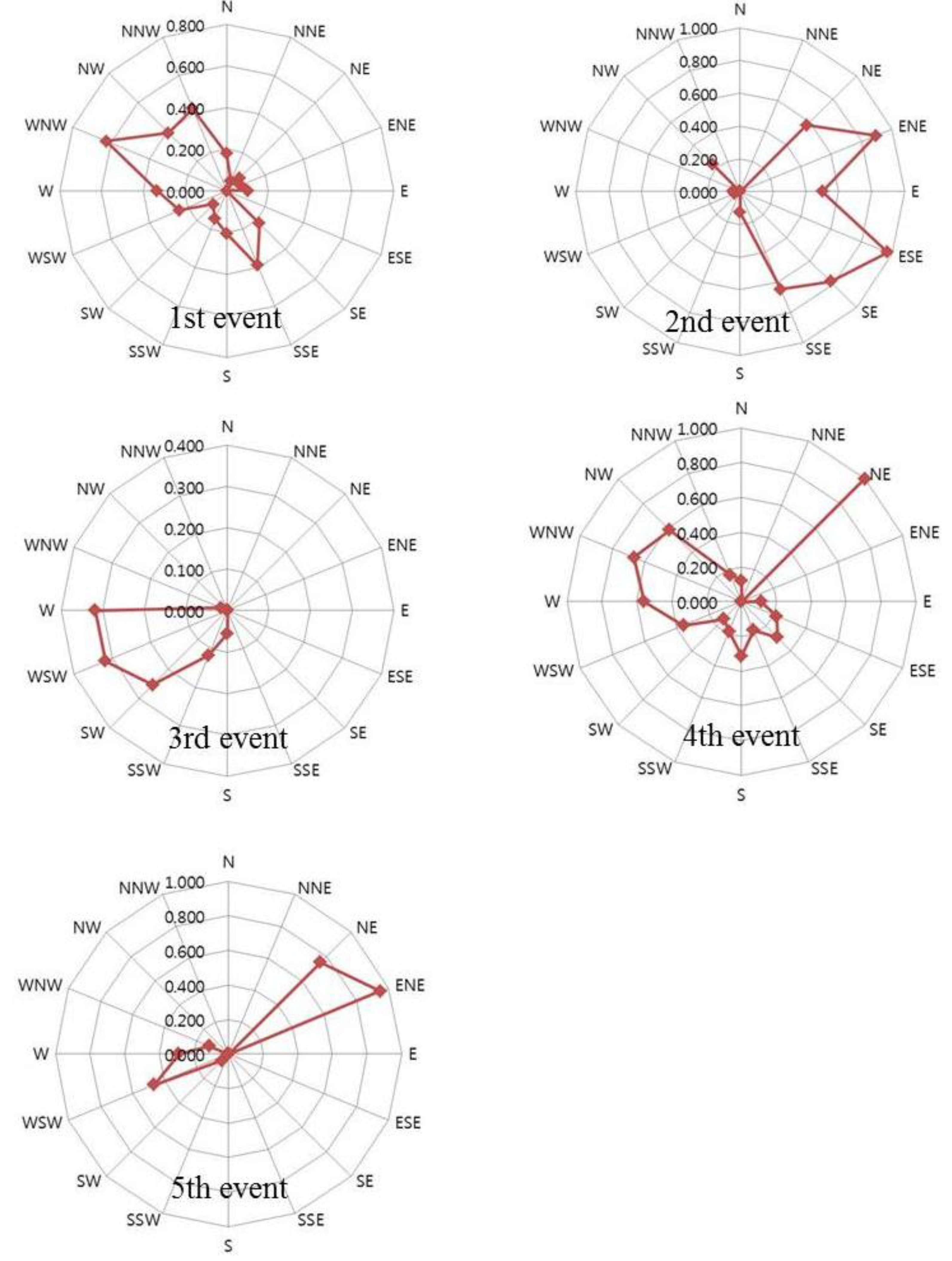
2.3. Impact of Local vs. Regional Sources

2.3.1. First Sampling Period

For the first sampling period (17–21 January 2013), TGM concentration was well correlated with SO2 and CO, but not with NO2 (Table 4). The atmospheric residence time of NO2 (1 day) is shorter than SO2 (3 days) or CO (60 days) [40]. The major source of NO2 in Korea is vehicle emission which contributes about 55% of the total NO2 emissions [41]. These results suggest that vehicles were not a major source of TGM for the first sampling period, and the good correlation of TGM with SO2 and CO suggests that coal combustion was important for enhancing TGM concentrations. CPF shows that the high TGM concentration occurred with NW and SE directions, indicating the possible effects of both Chinese and mainland Korean sources (Figure 5). Figure 6 also indicates that some back-trajectories for the top 10% TGM concentration samples for this period originated from mainland of Korea but most traveled through industrial areas of China (Shandong and Henan Provinces). Back-trajectories for the bottom 10% TGM concentration samples all passed through northern China originating in Mongolia (Figure 6). In total, these results suggest that both Korean and Chinese sources affected TGM concentration at the sampling site for this sampling period and likely sources include coal combustion.
Table 4. Pearson correlation coefficient (R) with four representative air pollutants for TGM and their corresponding concentrations for each sampling period. Correlation coefficients with an asterisk indicate statistically significant relationships at α = 0.05.
SO2NO2COO3
R (p-value)Conc. (ppb)R (p-value)Conc. (ppb)R (p-value)Conc. (ppm)R (p-value)Conc. (ppb)
1st Period0.474* (<0.001)5.76 ± 4.240.155 (0.078)26.71 ± 12.380.465* (<0.001)0.52 ± 0.17−0.135 (0.129)21.71 ± 13.54
2nd Period0.552* (<0.001)7.31 ± 3.020.558* (<0.001)28.84 ± 19.100.362* (0.001)0.65 ± 0.19−0.532* (<0.001)28.33 ± 14.67
3rd Period0.402* (<0.001)4.83 ± 1.680.304* (0.001)8.61 ± 3.330.543* (<0.001)0.35 ± 0.08−0.136 (0.162)46.76 ± 6.04
4th Period0.286* (0.003)5.67 ± 2.480.040 (0.684)17.18 ± 5.910.438* (<0.001)0.48 ± 0.110.224* (0.020)36.15 ± 19.40
5th Period0.161 (0.103)4.65 ± 1.590.254* (0.009)10.20 ± 3.760.484* (<0.001)0.50 ± 0.120.241* (0.014)40.93 ± 29.58
Total0.441* (<0.001)5.58 ± 2.980.560* (<0.001)18.22 ± 13.110.560* (<0.001)0.50 ± 0.16−0.242* (<0.001)34.53 ± 20.40

2.3.2. Second Sampling Period

Among the five sampling periods, the average TGM concentration was the highest for the second period and the coefficient of variation (the standard deviation divided by the arithmetic mean) was also high (Table 1, Figure 2), suggesting a higher influence of local sources compared to regional background contributions, since contributions from background sources are generally less variable than contributions from local sources [24,26,42,43,44]. During this period, TGM was statistically well correlated with SO2, NO2, and CO, with the Pearson correlation coefficient highest with NO2 (Table 4). The correlation coefficient between NO2 and CO was the highest during this period (0.47) relative to 0.21–0.37 for the other periods. Since the biggest source of NO2 and CO in Korea is vehicle exhaust emissions [41,45], these findings suggest that this source was one of the causes of the elevated TGM concentrations, along with coal-fired power plants. This conclusion is supported by the diel variation in TGM concentrations which had two major peaks during rush hour for only the second sampling period (Figure 4). The relatively lower correlation coefficient with CO than with NO2 and SO2 also suggests that the long-range transport from regional sources were not as important as local sources. For this period, a large number of back-trajectories passed through western mainland Korea (Figure 6). CPF also indicated that TGM concentration increased with easterly and southerly winds (Figure 5). Therefore, for the second sampling period, there is a high probability that mainland Korean vehicle emissions were the most important cause of enhanced TGM concentrations.
Figure 5. CPF (Conditional Probability Function) plot for each sampling period.
Atmosphere 05 00273 g005

2.3.3. Third Sampling Period

Among the five sampling periods, the lowest concentrations of TGM, NO2, and CO and the second lowest of SO2 were measured during the third sampling period (Table 4). NO2, representing local sources, had an average concentration of only 47% of all five sampling periods. For this period, the winds were consistently from the west (Figure 2) and TGM had the strongest correlation with CO; therefore, fossil fuel combustion in China was a likely major source. High TGM concentrations were associated with westerly winds in CPF analysis (Figure 5), and most of the back-trajectories originated from Northeastern China and did not pass through mainland Korea (Figure 6). A minimal effect from local sources was also indicated by the lowest coefficient of variation of 0.19 among the five sampling periods. Another notable fact is that a high wind speed (6.98 ± 2.56 m∙s−1) was observed; significantly larger than the average wind speed for other sampling periods (1.5 ± 1.4 m∙s−1) (Table 1). Generally, high wind speeds cause effective horizontal dilution in ambient air, leading to low TGM concentration; over the complete sampling period there was a statistically significant negative correlation between TGM concentration and wind speed (p-value < 0.001) (Table 3). To conclude, it is likely that Chinese emissions along with high wind speed and without local source contributions were responsible for the relatively low TGM concentrations observed during the third sampling period.

2.3.4. Fourth Sampling Period

During the fourth sampling period, TGM had a statistically significant correlation with SO2 and CO, but not with NO2, similar to the first sampling period. However, the back-trajectories did not pass through mainland Korean sources or industrial areas of China. Most trajectories stayed over the Yellow Sea for long periods of time (Figure 6). It is known that gaseous elemental mercury (GEM) is emitted from the natural surfaces, with the ocean being the largest natural source, contributing approximately 33% of total Hg emissions from both anthropogenic and natural sources [6]. According to Han et al. [46], the Atlantic Ocean was suggested to be a significant source of TGM measured in NY State, USA using back-trajectory based models. If the ocean was a significant source of TGM, concentrations should increase as solar radiation increases because Hg emissions are controlled primarily by a photo-reduction process initiated by solar radiation [47,48,49]. For the fourth sampling period, the correlation coefficient between TGM and solar radiation was the highest (r = 0.680) among all five sampling periods (Table 3), and TGM also was positively correlated with O3 (Table 4) which is produced by photochemical reactions. In addition, the diel pattern of TGM showed one major peak at noon (Figure 4) while the main peak appeared at 7–10 am for all other sampling periods. In addition, the increment from the nighttime minimum (at 20:00) to the daytime maximum (at 12:00) was the largest among the five sampling periods (Figure 4). These results altogether suggest that the volatilization of Hg from the ocean was an important source for this sampling period.
Since the YCPP was located approximately 4.5 km southwest of the sampling site TGM concentrations were expected to be enhanced during southwesterly winds if the impact of YCPP was significant. During this period, high TGM concentrations were regularly associated with wind directions between 180 and 315° (Figure 2 and Figure 5). The large coefficient of variation (0.36) for TGM concentrations suggests that TGM concentrations were influenced by local sources and local chemistry to a greater extent than regional sources during this period [50,51]. Therefore, in the fourth sampling period, both natural sources and the local YCPP source were important.

2.3.5. Fifth Sampling Period

During the fifth sampling period TGM had the strongest correlations with CO, followed by NO2 (Table 4), suggesting that both long-range transport and local sources concurrently affected TGM concentrations. The correlation coefficient between TGM and NO2 was weak, suggesting that vehicle emissions were not significant; in addition, no rush hour peaks for TGM were observed (Figure 4). During this period, the top 10% concentration samples were associated with distinctly different back-trajectories than the lowest 10% concentration samples. High concentration samples passed through Northern China, North Korea, and metropolitan areas of Korea (Figure 6). For the lowest 10% samples, all back-trajectories originated from the Yellow Sea (Figure 6). CPF also shows a relationship between winds from NE and high TGM concentrations (Figure 5). Unlike the ocean associated trajectories from period 4, which were associated with high concentrations, heavy rain occurred (precipitation depth = 75 mm) during the fifth sampling period (on 23 August 2013). Since the evasion of Hg from the water surface is primarily due to photoreduction initiated by solar radiation, heavy rain possibly inhibited the emission of Hg from the ocean surface and consequently caused low TGM concentrations in the ambient air [52] (Figure 2). Solar radiation measured during the fifth sampling period was much lower than that during the fourth sampling period (Table 1).
Figure 6. Back-trajectories during each sampling period. Red and blue points indicate top 10% and bottom 10% of TGM concentrations, respectively.
Atmosphere 05 00273 g006

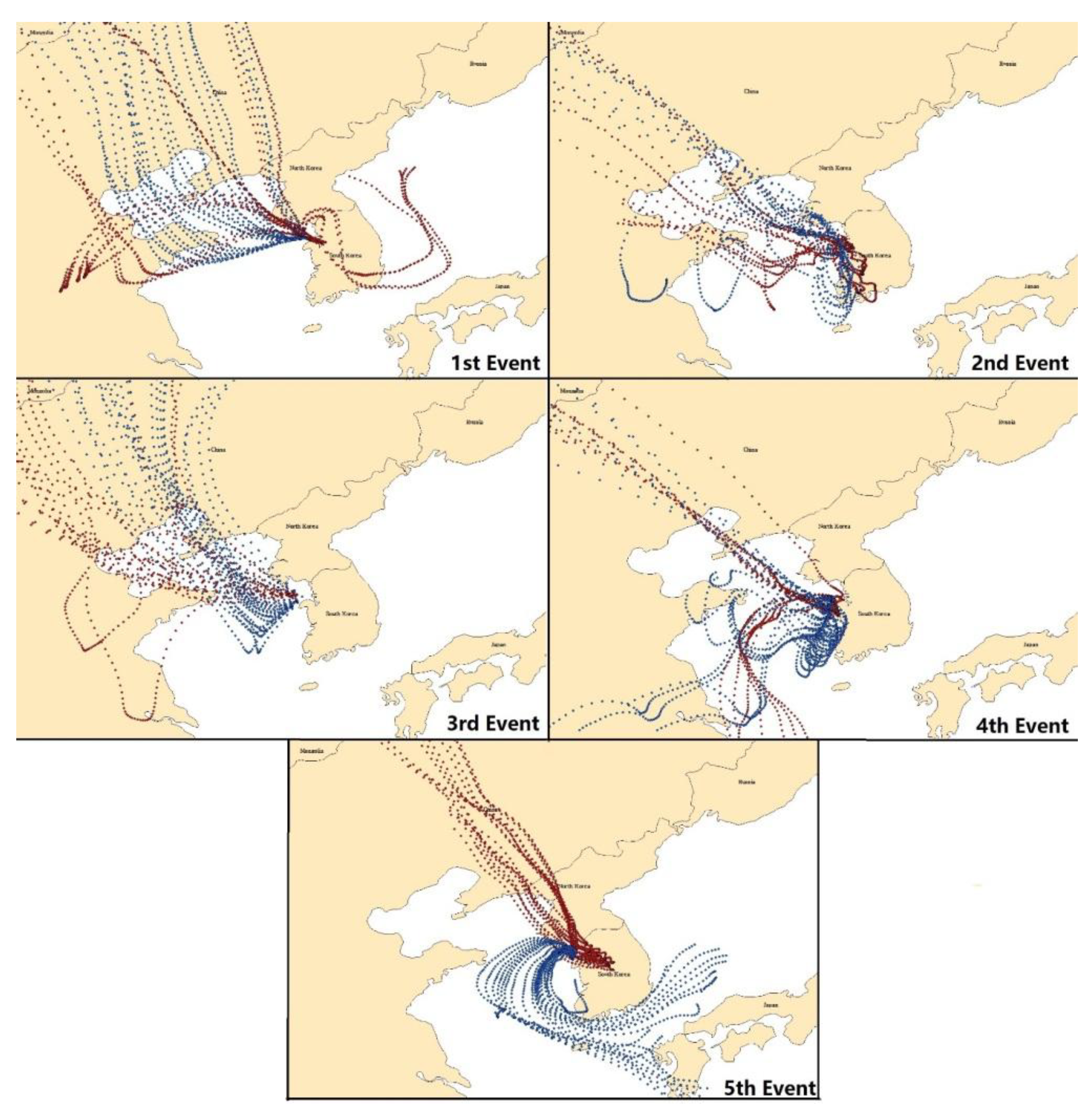
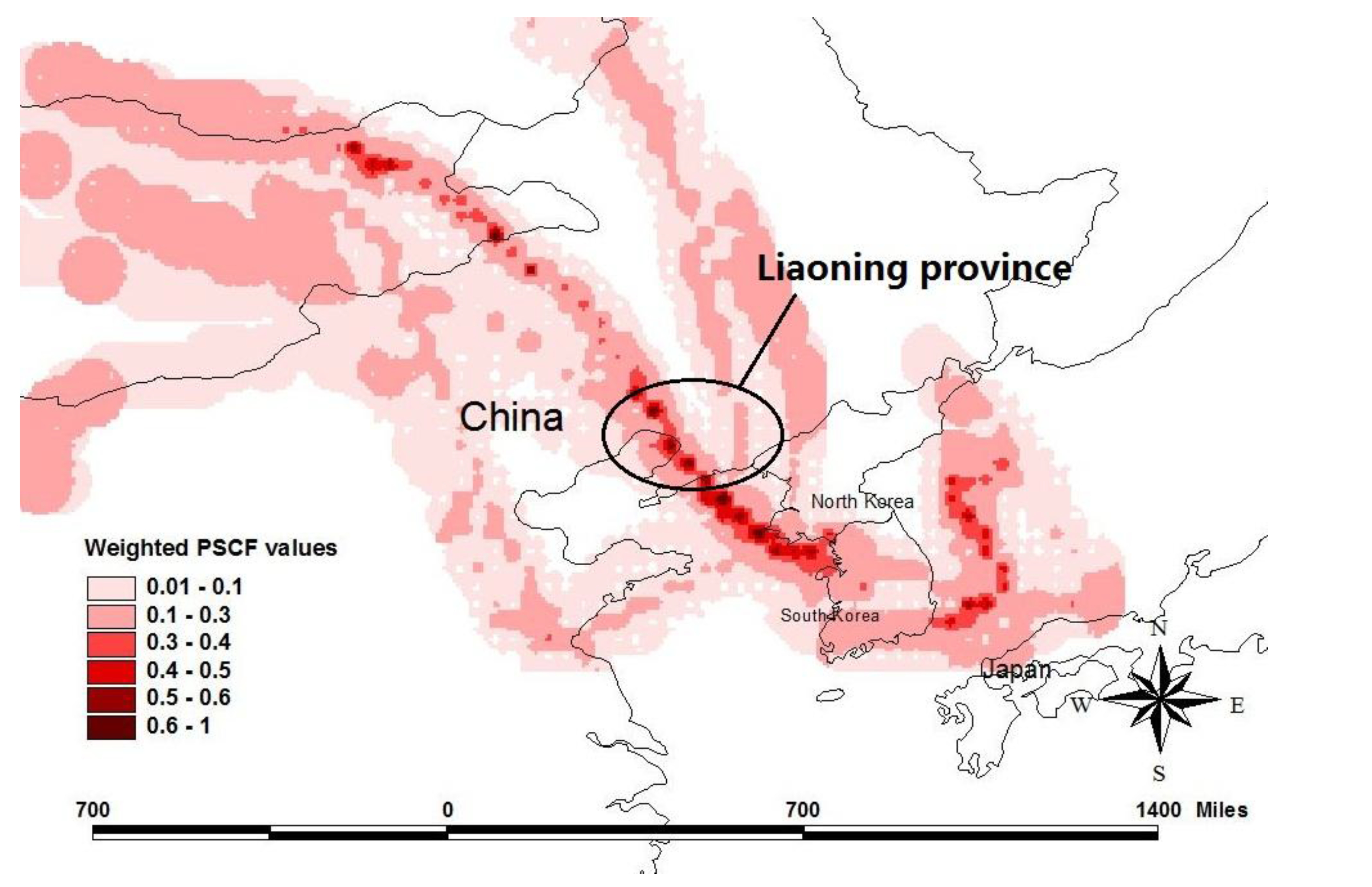
2.4. Potential Source Contribution Function

In order to identify the possible source areas associated with elevated TGM concentrations, potential source contribution function (PSCF) was used. Hourly back-trajectories were calculated for each hourly observation of TGM concentration. The number of back-trajectories was 540 for each arrival height of 200 m and 500 m. The criterion value used to distinguish between high and low concentrations was set to the top 25% value (4.29 ng∙m−3) to identify the larger sources. To reduce the uncertainty in a grid cell with a small number of endpoints, an arbitrary weight function Wij was applied when the number of the end points in a particular cell was less than three times the average number of end points (Nave) for all cells [35,46,53,54].
Atmosphere 05 00273 i001
PSCF combines both measurement data at the sampling site and meteorological data; therefore, sources outside the region of back-trajectory pathways are not identified. To indicate which areas would be included in the PSCF modeling, the total residence time of back-trajectories (total number of endpoints in each grid) is shown in Figure 6. The prevailing winds were generally from the east, and the west.
Potential source areas identified by the PSCF modeling include Liaoning province, the biggest Hg emitting province in China, which was linked to non-ferrous smelters [55] (Figure 7). The Yellow Sea and East Sea (Sea of Japan) were also identified as possible sources; however, it is not certain whether these areas were actual natural sources or appeared due to trailing effects. If the East Sea (Sea of Japan) area was caused by the trailing effect, the actual source is probably the southeastern industrial area of Korea, which was identified as a local mainland Korean source in Figure 7.
Figure 7. PSCF result for tracing regional sources. A grid cell size of 0.5° by 0.5° was used.
Atmosphere 05 00273 g007

3. Experimental Section

3.1. Sampling and Analysis

The sampling site was located on the roof of three-story building one Yongheung Island, Korea (lat: 37.15, lon: 126.28). Yongheung Island is a small island located about 15~20 km west from the mainland of Korea, having a population of 5815 according to a 2013 census. Tourism has been this Island’s main source of revenue. The Yongheung Coal-fired Power Plant (YCPP) was constructed in 2004, emitting about 0.11 ton∙yr−1 of Hg. The sampling site was located approximately 4.8 km northeast from the YCPP. At this site, TGM (GEM+GOM) was measured during five intensive periods in winter, spring, and summer in 2013 using a Tekran 2537B (Table 1). Outdoor air at a flow rate of 1.5 L∙min−1 was transported through a 3-m-long heated sampling line (1/4” OD Teflon) into the analyzer.
The Tekran 2537B underwent automated daily calibrations using an internal permeation source. Manual injections were also used to evaluate these automated calibrations before each sampling campaign using a saturated mercury vapor standard. The relative percent difference between manual injections and automated calibration was less than 2%. The method detection limit was calculated as three times the standard deviation obtained after injecting 1 pg of the mercury vapor seven times (0.04 ng∙m−3). The recovery rate was obtained by directly injecting Hg vapor into the sampling line between the sample inlet and the Tekran 2537B in a zero-air stream. It was between 85% and 110% (96 ± 3%). All Teflon products were acid-cleaned following EPA method 1631E before use.
Meteorological data including temperature, wind direction, wind speed, relative humidity, solar radiation, and precipitation depth were also measured every 5 min at the sampling site using a meteorological tower (DAVIS Inc weather station, Vintage Pro2TM). During the sampling period, the atmospheric temperature and wind speed ranged from −6.2 to 31.0 °C (9.6 ± 9.4°C) and 0.0 to 13.0 m∙s−1 (2.7 ± 2.8 m∙s−1).

3.2. Other Atmospheric Pollutants

The concentrations of NO2, SO2, CO, and O3 were obtained from the nearest national air quality monitoring station located approximately 8 km east from the sampling site. NO2, SO2, CO and O3 were measured by a chemiluminescent method, pulse UV florescence method, non-dispersive infrared method, and UV photometric method, respectively (http://www.airkorea.or.kr/). These concentrations were compared with those measured at another national air quality monitoring station located approximately 24 km west from the Hg sampling site, and there were no statistical difference (p-value < 0.001), indicating that the spatial distribution of these pollutants were relatively uniform across the area.

3.3. Backward Trajectory

The three-day backward trajectories were calculated using the NOAA HYSPLIT 4.7 with GDAS (Global Data Assimilation System) meteorological data. The GDAS archive has 3-hourly, global, 1 degree latitude longitude datasets of the pressure surface. In this study, hourly back-trajectories were calculated for each hourly averaged sample concentrations, and the arrival heights of 200 m and 500 m were used to describe the local and the regional transport meteorological pattern.

3.4. Conditional Probability Function

The conditional probability function (CPF), which is the conditional probability that a given concentration from a given wind direction will exceed a predetermined threshold criterion, was calculated as the following equation.
Atmosphere 05 00273 i002
where m∆θ is the number of occurrences from wind sector ∆θ where the TGM concentration is in the upper 25th percentile, and n∆θ is the total number of occurrence from this wind sector.

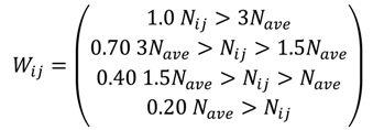
3.5. Potential Source Contribution Function

The PSCF model counts each trajectory segment endpoint that terminates within given grid cell. The probability of an event at the receptor site is related to the number of endpoints in that cell relative to the total number of endpoints for all of the sampling dates [56,57]. If N is the total number of trajectory endpoints over the study period and if n is the number of endpoints of trajectories falling in a given ijth cell, the probability of this event (P[Aij]) is calculated by nij/N. Also, if mij is the number of endpoints associated with higher concentration than a criterion value in ijth cell, the probability of this high concentration event, Bij, is given by P[Bij] of mij/N. ThePSCF value in a given grid ijth cell is then calculated using the following equation.
PSCF value = P[Bij]/P[Aij] = mij/nij
Grid cells containing sources enhancing the TGM concentration measured at the receptor site are recognized as possible source areas in PSCF. The criterion value used was the top 25% of TGM concentration, which is 4.29 ng∙m−3. The cell size of 0.5° by 0.5° was used for tracing sources. More detailed descriptions of the PSCF model are in previous publications [46,58].

4. Conclusions

TGM concentrations were measured in the farthest western island of Korea in between eastern China and mainland Korea in 2013 in order to identify important TGM sources to this location. In general, westerly and southwesterly winds were predominant during the sampling periods; however, the TGM concentration was not directionally dependent. TGM concentrations showed a distinct diel variation with higher values during the daytime than during the nighttime. Concentrations were generally positively correlated with solar radiation, indicating that volatilization of natural surfaces were significant.
Multiple tools including the relationship with other atmospheric pollutants, TGM diel variation, backward trajectories, and meteorological data were used to identify the relative impact of mainland Korean and regional Chinese sources on TGM concentrations at the sampling site for each of five sampling periods. For two periods (January and August 2013), TGM was found to be enhanced by both mainland Korean and regional Chinese coal-fired sources based on the good correlations with SO2 and CO and back-trajectories that passed through both mainland Korea and industrial areas of China. One period (February 2013) appeared to be affected by mainland vehicle emissions because TGM was significantly correlated with SO2, NO2, and CO and had two major peaks during rush hours. Also, a large number of back-trajectories originated from mainland Korea, suggesting that mainland Korean sources were important. During the April period, low concentrations and low coefficients of variation for TGM and other atmospheric pollutants associated with back-trajectories passing through China suggest that regional Chinese sources affected the TGM concentration. The very high wind speed observed in this sampling period was also an important factor for reducing atmospheric TGM concentrations. For the remaining sampling period (May 2013), a significant number of trajectories remained above the Yellow Sea (Eastern China Sea) and TGM concentration was significantly correlated with solar radiation, suggesting that TGM by volatilization from the ocean was important.
PSCF was also used to locate possible source areas. For mainland Korea sources, metropolitan areas (Seoul), the western coal-fired power plants area, and the southeast industrial area were identified as significant source areas. In addition, Liaoning province, the biggest Hg emitting province in China was found to be associated with increased TGM concentrations at the receptor site. These results highlight the need for international cooperation between Korea and China to reduce atmospheric Hg concentrations in Korea.

Acknowledgements

This work was supported by Basic Science Research Program through the National Research Foundation of Korea (NRF) funded by the Ministry of Education, Science, and Technology (2012R1A1A2042150).

Author Contributions

The work presented here was carried out in collaboration between all authors. Gang S. Lee analyzed data and wrote the paper. Pyung R. Kim performed the experiments and interpreted the results. Young J. Han defined the research theme, interpreted the results, and wrote the paper. Thomas M. Holsen also interpreted the results and approved the final paper. Seung H. Lee contributed to trajectory-based modeling.

Conflicts of Interest

The authors declare no conflict of interest.

References

  1. Driscoll, C.T.; Han, Y.J.; Chen, C.Y.; Evers, D.C.; Lambert, K.F.; Holsen, T.M.; Kamman, N.C.; Munson, R.K. Mercury contamination in forest and freshwater ecosystems in the Northeastern United States. Appl. Environ. Microbiol. 2007, 57, 17–28. [Google Scholar]
  2. Buehler, S.S.; Hites, R.A. The Great Lakes integrated atmospheric deposition network. Environ. Sci. Technol. 2002, 36, 354A–359A. [Google Scholar] [CrossRef]
  3. Landis, M.; Vette, A.F.; Keeler, G.J. Atmospheric mercury in the Lake Michigan Basin: Influence of the Chicago/Gary Urban Area. Environ. Sci. Technol. 2002, 36, 4508–4517. [Google Scholar] [CrossRef]
  4. Munthe, J. Recovery of mercury-contaminated fisheries. Ambio 2007, 36, 33–44. [Google Scholar] [CrossRef]
  5. Lyman, S.N.; Gustin, M.S.; Prestbo, E.M.; Kilner, P.I.; Edgerton, E.; Hartsell, B. Testing and application of surrogate surfaces for understanding potential gaseous oxidized mercury dry deposition. Environ. Sci. Technol. 2009, 43, 6235–6241. [Google Scholar] [CrossRef]
  6. UNEP. The Global Atmospheric Mercury Assessment; UNEP Chemicals Branch: Geneva, Switzerland, 2013. [Google Scholar]
  7. Schroeder, W.H.; Munthe, J. Atmospheric mercury—An overview. Atmos. Environ. 1998, 32, 809–822. [Google Scholar] [CrossRef]
  8. Zhang, L.; Gong, S.; Padro, J.; Barrie, L. A size-segregated particle dry deposition scheme for and atmospheric aerosol module. Atmos. Environ. 2001, 35, 549–560. [Google Scholar] [CrossRef]
  9. Fang, G.C.; Zhang, L.; Huang, C.S. Measurement of size-fractionated concentration and bulk dry deposition of atmospheric particulate bound mercury. Atmos. Environ. 2012, 61, 371–377. [Google Scholar] [CrossRef]
  10. Slemr, F.; Schuster, G.; Seiler, W. Distribution, speciation and budget of atmospheric mercury. J. Atmos. Chem. 1985, 3, 407–434. [Google Scholar]
  11. Seigneur, C; Vijayaraghavan, K.; Lohman, K.; Karamchandani, P.; Scott, C. Global source attribution for mercury deposition in the United States. Environ. Sci. Technol. 2004, 38, 555–569. [Google Scholar] [CrossRef]
  12. Jaffe, D.; Prestbo, E.; Swartzendruder, P.; Weiss-Penzias, P.; Kato, S.; Takami, A.; Hatakeyama, S.; Kaiji, Y. Export of atmospheric mercury from Asia. Atmos. Environ. 2005, 39, 3029–3038. [Google Scholar] [CrossRef]
  13. Obrist, D.; Gannet, H.A.; McCubbin, I.; Stephens, B.B.; Rahn, T. Atmospheric mercury concentrations at Storm Peak Laboratory in the Rocky Mountains: Evidence for long-range transport from Asia, boundary layer contributions, and plant mercury uptake. Atmos. Environ. 2008, 42, 7579–7589. [Google Scholar] [CrossRef]
  14. Kim, K.H.; Kim, M.Y. The effects of anthropogenic sources on temporal distribution characteristics of total gaseous mercury in Korea. Atmos. Environ. 2000, 34, 3337–3347. [Google Scholar] [CrossRef]
  15. Kim, K.H.; Kim, M.Y.; Kim, J.; Lee, G.W. The concentrations and fluxes of total gaseous mercury in a western coastal area of Korea during late March 2001. Atmos. Environ. 2002, 34, 3413–3427. [Google Scholar]
  16. Shon, Z.H.; Kim, K.H.; Song, S.K.; Kim, M.Y.; Lee, J.S. Environmental fate of gaseous elemental mercury at an urban monitoring site based on long-term measurements in Korea (1997–2005). Atmos. Environ. 2008, 42, 142–155. [Google Scholar] [CrossRef]
  17. Gan, S.Y.; Choi, E.M.; Seo, Y.S.; Yi, S.M.; Han, Y.J. Characteristic of atmospheric speciated mercury measured in Seoul, Chuncheon and Ganghwado. Korean Soc. Atmos. Environ. 2009, 5, 213–214. [Google Scholar]
  18. Nguyen, T.H.; Kim, M.Y.; Kim, K.H. The influence of long-range transport on atmospheric mercury on Jeju Island, Korea. Sci. Total Environ. 2010, 408, 1295–1307. [Google Scholar] [CrossRef]
  19. Kim, K.H.; Shon, Z.H.; Nguyen, H.T.; Jung, K.; Park, C.G.; Bae, G.N. The effect of man made source processes on the behavior of total gaseous mercury in air: A comparison between four urban monitoring sites in Seoul Korea. Sci. Total Environ. 2011, 409, 3801–3811. [Google Scholar] [CrossRef]
  20. Seo, Y.C. Personal Communication. Yonsei University: Seoul, Korea, 2007. [Google Scholar]
  21. AMAP/UNEP Technical Background Report on the Global Anthropogenic Mercury Assessment; Arctic Monitoring and Assessment Programme/UNEP Chemicals Branch: Geneva, Switzerland, 2008; p. 159.
  22. Kim, S.H.; Han, Y.J.; Holsen, T.M.; Yi, S.M. Characteristic of atmospheric speciated mercury concentrations (TGM, Hg(II) and Hg(p)) in Seoul, Korea. Atmos. Environ. 2009, 43, 3267–3274. [Google Scholar] [CrossRef]
  23. Cheng, I.; Zhang, L.; Mao, H.; Blanchard, P.; Tordon, R.; John, D. Seasonal and diurnal patterns of speciated atmospheric mercury at a coastal-rural and coastal-urban site. Atmos. Environ. 2014, 82, 193–205. [Google Scholar] [CrossRef]
  24. Valente, R.; Shea, C.; Lynn, H.K.; Tanner, R. Atmospheric mercury in the Great Smoky Mountains compared to regional and global levels. Atmos. Environ. 2007, 41, 1861–1873. [Google Scholar] [CrossRef]
  25. Han, Y.J.; Kim, J.E.; Kim, P.R.; Kim, W.J.; Yi, S.M.; Seo, Y.S.; Kim, S.H. General trends of Atmospheric mercury concentrations in urban and rural areas in Korea and characteristics of high-concentration events. Atmos. Environ. 2014. submitted. [Google Scholar]
  26. Kim, K.H.; Yoon, H.O.; Richard, J.C.B.; Jeon, E.C.; Sohn, J.R.; Jung, K.; Park, C.C.; Kim, I.S. Simultaneous monitoring of total gaseous mercury at four urban monitoring stations in Seoul, Korea. Atmos. Res. 2013, 132–133, 199–208. [Google Scholar] [CrossRef]
  27. Feng, X.; Yan, H.; Wang, S.; Qiu, G.; Tang, S.; Shang, L.; Dai, Q.; Hou, Y. Seasonal variation of gaseous mercury exchange rate between air and water surface over Baihua reservoir, Guizhou, China. Atmos. Environ. 2004, 38, 4721–4732. [Google Scholar] [CrossRef]
  28. Poissant, L.; Pilote, M.; Beauvais, C.; Constant, P.; Zhang, H.H. A year of continuous measurements of three atmospheric mercury species (GEM, RGM and Hgp) in southern Quebec, Canada. Atmos. Environ. 2005, 39, 1275–1287. [Google Scholar] [CrossRef]
  29. Choi, H.D.; Holsen, T.M.; Hopke, P.K. Atmospheric mercury in the Adirondacks: Concentrations and sources. Environ. Sci. Technol. 2008, 42, 5644–5653. [Google Scholar] [CrossRef]
  30. Amyot, M.; Auclair, J.C.; Poissant, L. In situ high temporal resolution analysis of elemental mercury in natural waters. Anal. Chimica Acta 2001, 447, 153–159. [Google Scholar] [CrossRef]
  31. O’Driscoll, N.J.; Siciliano, S.D.; Lean, D.R.S. Continuous analysis of dissolved gaseous mercury in freshwater lakes. Sci. Total Environ. 2003, 304, 285–294. [Google Scholar] [CrossRef]
  32. Choi, H.D.; Holsen, T.M. Gaseous mercury emission from the forest floor of the Adirondacks. Environ. Pollut. 2009, 157, 592–600. [Google Scholar] [CrossRef]
  33. Choi, E.M.; Kim, S.H.; Holsen, T.M.; Yi, S.M. Total gaseous concentration in mercury in Seoul, Korea: Local sources compared to long-range transport from China and Japan. Environ. Pollut. 2009, 157, 816–822. [Google Scholar] [CrossRef]
  34. Li, Z.; Xia, C; Wang, X.; Xiang, Y.; Xie, Z. Total gaseous mercury in Pearl River Delta region, China during 2008 winter period. Atmos. Environ. 2011, 45, 834–838. [Google Scholar] [CrossRef]
  35. Fu, X.; Feng, X.; Qiu, G.; Shang, L.; Zhang, H. Speciated atmospheric mercury and its potential source in Guiyang, China. Atmos. Environ. 2011, 45, 4205–4212. [Google Scholar] [CrossRef]
  36. Liu, S.; Nadim, F.; Perkins, C.; Carley, R.J.; Hoag, G.E.; Lin, Y.; Chen, L. Atmospheric mercury monitoring survey in Beijing, China. Chemosphere 2002, 48, 97–107. [Google Scholar] [CrossRef]
  37. Huang, J.; Liu, C.K.; Huang, C.S.; Fang, G.C. Atmospheric mercury pollution at an urban site in central Taiwan: Mercury emission sources at ground level. Chemosphere 2012, 87, 579–585. [Google Scholar] [CrossRef]
  38. Lyman, S.N.; Gustin, M.S. Determinants of atmospheric mercury concentrations in Reno, Nevada, U.S.A. Sci. Total Environ. 2009, 408, 431–438. [Google Scholar] [CrossRef]
  39. Lyman, M.M.; Keeler, G.J. Source-receptor relationships for atmospheric mercury in urban Detroit, Michigan. Atmos. Environ. 2006, 40, 3144–3155. [Google Scholar] [CrossRef]
  40. Hidy, G.M. Atmospheric Sulfur and Nitrogen Oxides: Eastern North America Source-Receptor Relationships; Academic Press Inc.: San Diego, CA, USA, 1994; p. 447. [Google Scholar]
  41. Pandey, S.K.; Kim, K.H.; Chung, S.Y.; Cho, S.J.; Kim, M.Y.; Shon, Z.H. Long term study of NOx behavior at urban roadside and background locations in Seoul, Korea. Atmos. Environ. 2008, 42, 607–622. [Google Scholar] [CrossRef]
  42. Lee, D.S.; Dollard, G.J.; Pepler, S. Gas-phase mercury in the atmosphere of the United Kingdom. Atmos. Environ. 1998, 32, 855–864. [Google Scholar] [CrossRef]
  43. Han, Y.-J.; Holsen, T.M.; Hopke, P.K.; Cheong, J.-P.; Kim, H.; Yi, S.-M. Identification of source locations for atmospheric dry deposition of heavy metals during yellow-sand events in Seoul, Korea in 1998 using hybrid receptor models. Atmos. Environ. 2004, 38, 5353–5361. [Google Scholar] [CrossRef]
  44. Chen, L.; Liu, M.; Fan, R.; Ma, S.; Xu, Z.; Ren, M.; He, Q. Mercury speciation and emission from municipal solid waste incinerators in the Pearl River Delta, South China. Sci. Total Environ. 2013, 447, 396–402. [Google Scholar] [CrossRef]
  45. Kim, K.H.; Shon, Z.H. Nationwide shift in CO concentration levels in urban areas of Korea after 2000. J. Hazard Mater. 2011, 188, 235–246. [Google Scholar] [CrossRef]
  46. Han, Y.J.; Holsen, T.M.; Hopke, P.K. Estimation of source location of total gaseous mercury measured in New York State using trajectory-based models. Atmos. Environ. 2007, 41, 6033–6047. [Google Scholar]
  47. Zhang, H.; Lindberg, S.E. Sunlight and iron (III)-induced photochemical production of dissolved gaseous mercury in freshwater. Environ. Sci. Technol. 2001, 5, 928–935. [Google Scholar] [CrossRef]
  48. Siciliano, S.D.; O’Driscoll, N.J.; Lean, D.R.S. Microbial reduction and oxidation of mercury in freshwater lakes. Environ. Sci. Technol. 2002, 36, 3064–3067. [Google Scholar] [CrossRef]
  49. Ahn, M.C.; Kim, B.C.; Holsen, T.M.; Yi, S.M.; Han, Y.J. Factor influencing concentrations of dissolved gaseous mercury (DGM) and total mercury (TM) in an artificial reservoir. Environ. Pollut. 2010, 158, 347–355. [Google Scholar] [CrossRef]
  50. Han, Y.J.; Holsen, T.M.; Lai, S.O.; Hopke, P.K.; Yi, S.M.; Liu, W.; Pangano, J.; Falanga, L.; Milligan, M.; Andolina, C. Atmospheric gaseous mercury concentration in New York State: relationships with meteorological data and other pollutants. Atmos. Environ. 2004, 38, 6431–6446. [Google Scholar] [CrossRef]
  51. Chen, L.; Liu, M.; Xu, Z.; Fan, R.; Tao, J.; Chen, D.; Zhang, D.; Xie, D.; Sun, J. Variation trends and influencing factors of total gaseous mercury in the Pearl River Delta-A highly industrialised region in South China influenced by seasonal monsoons. Atmos. Environ. 2013, 77, 757–766. [Google Scholar] [CrossRef]
  52. Fu, X.; Feng, X.; Wan, Q.; Meng, B.; Yan, H.; Guo, Y. Probing Hg evasion from surface waters of two Chinese hyper/meso-eutrophic reservoirs. Sci. Total Environ. 2010, 408, 5887–5896. [Google Scholar] [CrossRef]
  53. Polissar, A.V.; Hopke, P.K.; Harris, J.M. Source regions for atmospheric aerosol measured at Barrow, Alaska. Environ. Sci. Technol. 2001, 35, 4214–4226. [Google Scholar] [CrossRef]
  54. Polissar, A.V.; Hopke, P.K.; Poirot, R.L. Atmospheric aerosol over Vermont: Chemical composition and sources. Environ. Sci. Technol. 2001, 35, 4604–4621. [Google Scholar] [CrossRef]
  55. Fu, X.; Feng, X.; Sommar, J.; Wang, S. A review of studies on atmospheric mercury in China. Sci. Total Environ. 2012, 421–422, 73–81. [Google Scholar] [CrossRef]
  56. Ashbaugh, L.L.; Malm, W.C.; Sadeh, W.D. A residence time probability analysis of sulfur concentrations at Grand Canyon National Park. Atmos. Environ. 1985, 19, 1263–1270. [Google Scholar]
  57. Malm, W.C.; Johnson, C.E.; Bresch, J.F. Application of principal component analysis for purposes of identifying source-receptor relationships in receptor methods for source apportionment. In Receptor Methods for Source Apportionment; Air Pollution Control Association: Pittsburgh, PA, USA, 1986; pp. 127–148. [Google Scholar]
  58. Han, Y.J. Mercury in New York State: Concentrations and Source Identification Using Hybrid Receptor Modeling. Ph.D. Thesis, Clarkson University, Potsdam, NY, USA, 2003. [Google Scholar]

