Deployment and Evaluation of a Network of Open Low-Cost Air Quality Sensor Systems

Abstract

Low-cost air quality sensors have the potential to complement the regulatory network of air quality monitoring stations, with respect to increased spatial density of observations, however, their data quality continues to be of concern. Here we report on our experience with a small network of open low-cost sensor systems for air quality, which was deployed in the region of Stavanger, Norway, under Nordic winter conditions. The network consisted of AirSensEUR sensor systems, equipped with sensors for, among others, nitrogen dioxide and fine particulate matter. The systems were co-located at an air quality monitoring station, for a period of approximately six weeks. A subset of the systems was subsequently deployed at various roadside locations for half a year, and finally co-located at the same air quality monitoring station again, for a post-deployment evaluation. For fine particulate matter, the co-location results indicate a good inter-unit consistency, but poor average out-of-the-box performance (R² = 0.25, RMSE = 9.6 $\mathsf{\mu }$g m${}^{-3}$). While Köhler correction did not significantly improve the accuracy in our study, filtering for high relative humidity conditions improved the results (R² = 0.63, RMSE = 7.09 $\mathsf{\mu }$g m${}^{-3}$). For nitrogen dioxide, the inter-unit consistency was found to be excellent, and calibration models were developed which showed good performance during the testing period (on average R² = 0.98, RMSE = 5.73 $\mathsf{\mu }$g m${}^{-3}$), however, due to the short training period, the calibration models are likely not able to capture the full annual variability in environmental conditions. A post-deployment co-location showed, respectively, a slight and significant decrease in inter-sensor consistency for fine particulate matter and nitrogen dioxide. We further demonstrate, how observations from even such a small network can be exploited by assimilation in a high-resolution air quality model, thus adding value to both the observations and the model, and ultimately providing a more comprehensive perspective of air quality than is possible from either of the two input datasets alone. Our study provides valuable insights on the operation and performance of an open sensor system for air quality, particularly under challenging Nordic environmental conditions.

1. Introduction

Low-cost sensor systems for air quality applications are seeing increasing interest, in both research applications and citizen science frameworks [1,2,3]. They provide measurements with lower costs, improving the spatial coverage of the air pollution monitoring networks due to their portability and compact size. The observations made by such low-cost sensor systems can typically not reach the stability and accuracy of reference or reference-equivalent instrumentation [4,5]. In parallel to the emergence of standards for evaluating the performance of low-cost sensor systems [6], concerns regarding the low-cost sensors’ data quality have been reflected in extensive research for evaluating low-cost sensors under different environmental settings. Raw data obtained by the sensor systems can be processed [7,8,9,10], to substantially improve the data quality, and thus the usability for various applications [11,12,13,14,15,16,17]. However, in doing so, one should be aware that at some point a line is crossed, from independent measurements to statistical modelling [8,18,19].

Depending on the phase of air pollutants, low-cost sensors for monitoring air pollution benefit from various technologies and calibration approaches. Conductometric (resistive), capacitive, electrochemical, and resonant frequency (of the acoustic wave) devices are widely used for measuring gaseous pollutant concentrations [16]. The output of gaseous pollutant low-cost sensors is usually voltage or resistance instead of concentration [20]. For those sensor systems, the methodology for conversion from raw quantities to concentrations, therefore, remains the user’s choice. The sensor manufacturers provide limited data and methodological details for modifying raw gaseous sensor output, and the provided data are mainly derived under well-controlled laboratory conditions [20,21]. Numerous environmental parameters, such as the presence of other gaseous pollutants (gas cross-sensitivity) or ambient temperature/pressure variations, can influence the raw output of gaseous pollutant low-cost sensors [22,23]. For example, a review of previous work on the laboratory performance of nitrogen dioxide (NO₂) low-cost sensors, showed a median squared Pearson correlation coefficient, between sensor output and reference-grade instruments, (Corr2) approximately equal to 1.00 (n = 8 studies), while this value was 0.57 (Q1 = 0.24, Q2 = 0.84) for the outdoor performance of NO₂ sensors (n = 59) [5]. Ambient temperature and cross-sensitivity with other gaseous pollutants, in particular, ozone (O₃), substantially impact the performance of the NO₂ sensors [24]. Accordingly, correction and conversion of gaseous pollutant low-cost sensors’ measured voltage to concentrations, under field conditions, remain challenging in the sensor community.

Commercial particle pollutants low-cost sensors typically operate based on the light scattering principle, detecting the particles with aerodynamic diameters of 0.3–10 $\mathsf{\mu }$m. The particulate matter (PM) within an air flow is directed to a canal, passing across a beam of infrared or visible light. The scatter of the beam forms the basis for estimating the particle mass concentration. Compared to gaseous pollutant low-cost sensors, cross-sensitivity and long-term sensor drift are less problematic [25]; however, previous work has uncovered two shortcomings of most commercially available low-cost PM sensors in field conditions: (1) the estimated mass concentration of PM_2.5 (PM ≤ 2.5 $\mathsf{\mu }$m) is typically more accurate than PM₁₀, compared to reference-grade measurements [26,27,28]; and (2) high ambient relative humidity has a deteriorating impact on the PM sensor performance for most, but not all, low-cost PM sensors [4,29,30]. Low-cost PM sensors can exhibit variable accuracy due to different particle properties [31,32]; on the other hand, growth by water vapor (hygroscopic growth), due to high levels of relative humidity [33,34], leads to higher scattering of the light beam in the sensor chamber—overestimating the particle mass concentration. As a result, a wide range of approaches for calibration and post-processing of PM sensor data have been adopted [2]. Yet, these approaches are sensor/case-specific, and there is no universal solution for correcting PM sensor data [35,36].

To characterize the reliability of low-cost air pollution sensor systems in Nordic climatic conditions, we report here on the calibration, evaluation, and operation of a small network of co-located outdoor air quality sensor systems, which was deployed in the area of Stavanger, Norway. The network consists of AirSensEUR systems, that follow a completely open and transparent design [37,38,39]. AirSensEUR is an open low-cost air quality sensor platform developed by Libera Intentio (https://airsenseur.org/, accessed on 23 February 2023), in collaboration with the European Commission’s Joint Research Centre [40,41,42]. The systems can be configured to measure various pollutants; we focus here primarily on observations of NO₂ and PM_2.5, air pollutants of primary concern in Nordic countries [43,44]. While AirSensEUR systems have been evaluated in the field before [45,46,47], to the best of our knowledge no studies have been published on the deployment, calibration, and evaluation of a network of AirSensEUR systems under challenging Nordic environmental conditions.

The manuscript is structured as follows: Section 2 provides an overview of the sensors systems, the reference station, the calibration and correction algorithms, and a technique for data assimilation. Subsequently, Section 3 presents the results and discusses the findings. Finally, Section 4 gives a summary of the study and provides conclusions.

2. Data and Methodology

2.1. Sensors and Network

A total of ten AirSensEUR devices were evaluated in this study. These units were equipped with gas sensors for nitrogen dioxide (Alphasense NO2-B43F), carbon monoxide (Alphasense CO-A4), nitric oxide (Alphasense NO-B4), carbon dioxide (ELT D-300), and ozone (Alphasense OX-A431). In addition, the systems were equipped with an Alphasense OPC-N3 optical particle counter, that provides particle count in 24 size bins, as well as PM₁₀, PM_2.5, and PM₁ mass concentrations (in units of $\mathsf{\mu }$g m${}^{-3}$), using a factory calibration with constant particle density. Furthermore, each unit has sensors for air temperature, relative humidity, and atmospheric pressure. In this study, only the measurements from NO2-B43F, NO-B4, and OPC-N3, as well as temperature and relative humidity, were used. All gas sensors provide their raw output in digital numbers (DN) and need to be calibrated/converted to geophysical concentration units, such as $\mathsf{\mu }$g m${}^{-3}$.

These ten systems were first co-located for approximately five weeks at the Schancheholen air quality monitoring site in Stavanger, Norway. The Schancheholen air quality monitoring station (located at 58.95188${}^{\circ }$ N, 5.72188${}^{\circ }$ E ) is a roadside station, located to the side of the busy E39 highway, in the city of Stavanger. It represents an area with dense traffic, and pollution levels can be expected to be comparatively high. The station is equipped with a Grimm EDM180 dust monitor and Teledyne API T200 NO_x-monitor. Figure 1 shows the Schancheholen station with the ten AirSensEUR units mounted on top of it, for the co-location study. The co-location period was from 9 October 2019 to 17 November 2019.

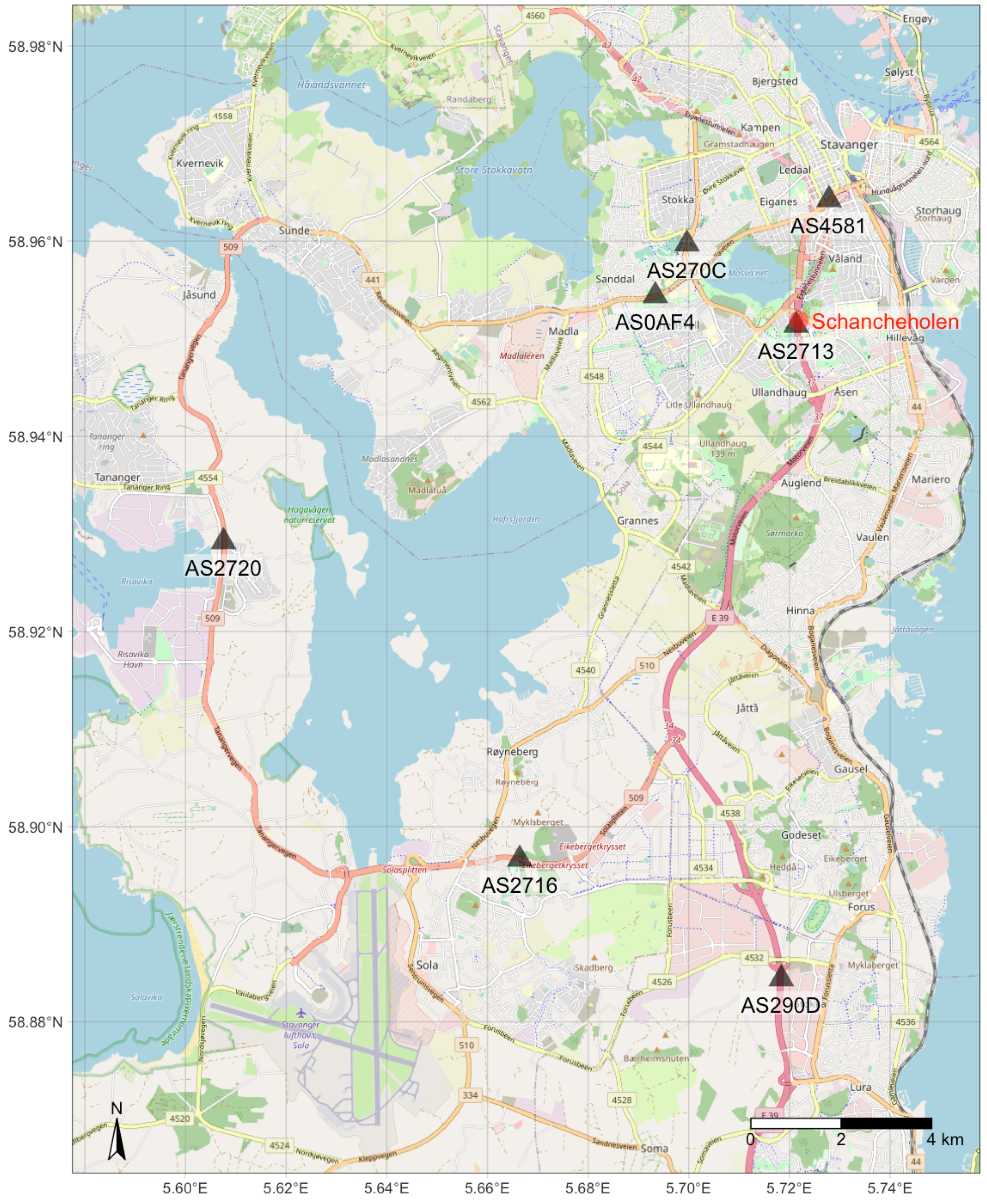
Subsequently, seven of the ten systems were deployed to various roadside locations south of Stavanger. Two sensor systems were deployed in the Haugesund area, northwest of Stavanger, but these were not further considered here due to the distance. Figure 2 shows a map of both the deployment sites and the location of the Schancheholen air quality monitoring station. The geographic coordinates of the final deployment sites can be found in

Table 1. Geographic coordinates of the locations for the seven deployed sensor units, given in decimal degrees (DD) on the WGS84 datum.

Sensor ID	Latitude [DD]	Longitude [DD]
AS0AF4	58.95441° N	5.69336° E
AS270C	58.95972° N	5.69963° E
AS2713	58.95138° N	5.72131° E
AS290D	58.88441° N	5.71838° E
AS2716	58.89665° N	5.66640° E
AS2720	58.92921° N	5.60756° E
AS4581	58.96425° N	5.72786° E

. The deployment period was from 18 November 2019 to 25 May 2020. One sensor system (AS2713) remained at the Schancheholen station throughout the entire deployment period.

2.2. Calibration for NO₂

A basic calibration procedure was carried out for NO₂. In principle, the digital numbers reported by the sensors (numeric range of 0 to 65,535) should be converted to voltage and current first, using platform-specific constants, before fitting a linear regression against the station-based observations [38,40]. Here, we tested the possibility of using the sensor-reported digital numbers directly in the regression. The calibration was carried out using the sensors NO2B43F (NO₂), NOB4 (NO), and temperature, as predictor variables, according to the following multilinear regression equation:

$$N{O}_2=a_0+a_1·NO2B43F+a_2·log\left(NOB4\right)+a_3·log(50+T)$$

(1)

where $N{O}_2$ is the NO₂ concentration in $\mathsf{\mu }$g m${}^{-3}$, $a_0$ through $a_3$ are the regression coefficients (unitless), $NO2B43F$ and $NOB4$ are the raw DN values of the sensors (unitless), and T is the measured temperature, in units of ${}^{\circ }$C. Both $NOB4$ and temperature were log-transformed after empirical testing. A constant of 50 was added to the temperature before transformation, to avoid mathematically undefined values for temperatures below 0 ${}^{\circ }$C.

As a training period, the first 70% of the data were used (9 October 2019 through 5 November 2019), whereas the remaining 30% of the data were used for testing the calibration (6 November 2019 through 16 November 2019).

Table 2. Multilinear regression coefficients for all sensor systems.

ID	Term	Estimate	Std. Error	t Value	p Value
AS2716	(Intercept)	16,467.95	188.04	87.58	0.000
AS2716	NO2B43F	−0.26	0.00	−90.76	0.000
AS2716	log(NOB4)	17.75	2.89	6.15	0.000
AS2716	log(50 + temperature)	−77.06	3.52	−21.91	0.000
AS270C	(Intercept)	12,239.40	343.55	35.63	0.000
AS270C	NO2B43F	−0.20	0.01	−35.92	0.000
AS270C	log(NOB4)	20.92	4.65	4.50	0.000
AS270C	log(50 + temperature)	52.45	9.53	5.50	0.000
AS4581	(Intercept)	14,850.42	215.67	68.86	0.000
AS4581	NO2B43F	−0.25	0.00	−70.94	0.000
AS4581	log(NOB4)	32.17	3.35	9.61	0.000
AS4581	log(50 + temperature)	33.33	5.09	6.55	0.000
AS2709	(Intercept)	14,796.37	378.20	39.12	0.000
AS2709	NO2B43F	−0.24	0.01	−39.22	0.000
AS2709	log(NOB4)	−11.38	4.59	−2.48	0.013
AS2709	log(50 + temperature)	48.15	8.63	5.58	0.000
AS2713	(Intercept)	12,907.25	196.38	65.73	0.000
AS2713	NO2B43F	−0.22	0.00	−65.53	0.000
AS2713	log(NOB4)	95.16	2.41	39.48	0.000
AS2713	log(50 + temperature)	13.91	5.52	2.52	0.012
AS290D	(Intercept)	15,154.54	183.92	82.40	0.000
AS290D	NO2B43F	−0.25	0.00	−82.31	0.000
AS290D	log(NOB4)	37.18	2.11	17.61	0.000
AS290D	log(50 + temperature)	−21.54	4.31	−5.00	0.000
AS6606	(Intercept)	15,664.17	163.55	95.78	0.000
AS6606	NO2B43F	−0.25	0.00	−96.20	0.000
AS6606	log(NOB4)	7.42	2.16	3.43	0.001
AS6606	log(50 + temperature)	16.35	4.34	3.77	0.000
AS0AF4	(Intercept)	17,344.91	211.91	81.85	0.000
AS0AF4	NO2B43F	−0.27	0.00	−84.95	0.000
AS0AF4	log(NOB4)	−8.76	3.35	−2.61	0.009
AS0AF4	log(50 + temperature)	−90.21	3.52	−25.63	0.000
AS2720	(Intercept)	15,190.69	263.70	57.61	0.000
AS2720	NO2B43F	−0.25	0.00	−58.60	0.000
AS2720	log(NOB4)	10.44	3.66	2.85	0.004
AS2720	log(50 + temperature)	−0.30	5.61	−0.05	0.957
AS6603	(Intercept)	12,307.27	259.40	47.44	0.000
AS6603	NO2B43F	−0.21	0.00	−50.27	0.000
AS6603	log(NOB4)	73.15	4.70	15.57	0.000
AS6603	log(50 + temperature)	19.86	6.61	3.00	0.003

provides the calibration coefficients as well as the corresponding statistics.

2.3. Humidity Correction for PM_2.5

For this study, we adapt and evaluate the proposed humidity correction from [33], which was developed for the Alphasense OPC-N2 PM sensor. The idea behind this correction is that, when water vapor molecules interact with aerosol particles, they can be adsorbed to the surface of the particles or absorbed into the bulk of the particles [48]. Depending on the characteristics of the particle, the uptake of water vapor can lead to aqueous solution droplet formation and a substantial increase in the particle diameter, where the growth by water vapor (hygroscopic growth) can be described by the so-called Köhler theory. The Köhler theory combines the Kelvin equation, for the dependence of vapor pressure on the curvature and surface tension of a liquid droplet, and Raoult’s law formulations of vapor pressure of aqueous solutions [49]. Based on this theory, [33] derived a correction factor C (unitless) to account for the relative humidity (RH) (in percent) effect on PM measurement as follows:

$$P{M}_{corrected}=P{M}_{raw}/C$$

(2)

$$C=1+\frac{\frac{\kappa }{1.65}}{-1+\frac{1}{a_w}}$$

(3)

where $P{M}_{corrected}$ and $P{M}_{raw}$ are the corrected and observed PM mass concentrations in units of $\mathsf{\mu }$g m${}^{-3}$, respectively, $a_w$ is the water activity (unitless), defined as RH/100, and $\kappa$ is 0.4 (unitless).

2.4. Assimilation of Sensor Observations in a Model

One promising application of sensor networks (although ideally much denser networks than the relatively small one used here) is high-resolution mapping of urban air quality, in real-time [50,51]. While it can be possible to simply use standard spatial interpolation techniques, such as inverse-distance weighting or ordinary kriging, when the sensor network is extremely dense (e.g., one sensor per 50 m by 50 m area) and/or the pollutant in question does not exhibit very steep spatial gradients (e.g., PM_2.5), such direct interpolation under more typically encountered network densities generally does not lead to realistic spatial patterns, but provides overly smooth results.

The most obvious solution to this problem, is to use the output from a physical model as an a priori dataset, and to use it for guiding the interpolation between the sensor observations. This can be done using a wide variety of techniques, most of which are still at the very forefront of research when it comes to applying them for high-reslution urban-scale air quality mapping. Previously, geostatistical methods have been used for combining the two datasets [13,50], but data assimilation methods stemming from a long heritage in numerical weather prediction are currently under consideration [51]. Data assimilation [52,53,54] is a set of powerful statistical techniques for integrating the information from observations in geophysical models. The output of a data assimilation procedure (the “analysis”) adds value to both the observations and the model. The observations are interpolated in space in a physically meaningful way, whereas the model is corrected for eventual biases.

Here, we use a conceptually simple data assimilation technique called Optimal Interpolation (OI) [52]. OI calculates the analysis vector ${\mathbf{x}}_a$ as (following the notation by Kalnay [54])

$${\mathbf{x}}_a={\mathbf{x}}_b+\mathbf{W}\left[{\mathbf{y}}_0-\mathit{H}\left({\mathbf{x}}_b\right)\right]$$

(4)

where ${\mathbf{x}}_b$ is the background field vector (i.e., here the output from the dispersion model), $\mathbf{W}$ is the matrix of weights, ${\mathbf{y}}_0$ is the set of observations obtained from the low-cost sensor network, and $\mathit{H}$ is the observation operator that converts values from the background into observation space (this is carried out here using simple bilinear interpolation). Subsequently, the matrix of weights $\mathbf{W}$ is computed as

$$\mathbf{W}=\mathbf{B}{\mathbf{H}}^{\mathbf{T}}{\left(\mathbf{R}+{\mathbf{HBH}}^{\mathbf{T}}\right)}^{-1}$$

(5)

where $\mathbf{B}$ is the background error covariance matrix, the matrix $\mathbf{H}$ is the linear tangent perturbation of $\mathit{H}$, and $\mathbf{R}$ is the matrix of observation error covariances (which is diagonal in our case, as the observation errors at different locations are assumed to be uncorrelated). Furthermore, if required, the analysis error covariance ${\mathbf{P}}_a$ can be computed as

$${\mathbf{P}}_a=\left(\mathbf{I}-\mathbf{WH}\right)\mathbf{B}$$

(6)

where $\mathbf{I}$ is the identity matrix. The background error covariance matrix $\mathbf{B}$ was generated here as a function of both distance and the pixel-to-pixel similarity within the modeled air quality field. As the values in the $\mathbf{B}$ matrix are prescribed, they are potentially suboptimal [52,54]. As model information, we used output from the uEMEP model [55,56], provided by the Norwegian Meteorological Institute.

3. Results and Discussion

3.1. Pre-Deployment Co-Location

In the following sections we present the evaluation results obtained during the field co-location at the Schancheholen air quality monitoring station. We first show results for PM_2.5 and then for NO₂. PM₁₀ was not considered here, given that the measurement principle typically does not allow measurements of coarser particles [27].

3.1.1. Evaluation of PM_2.5

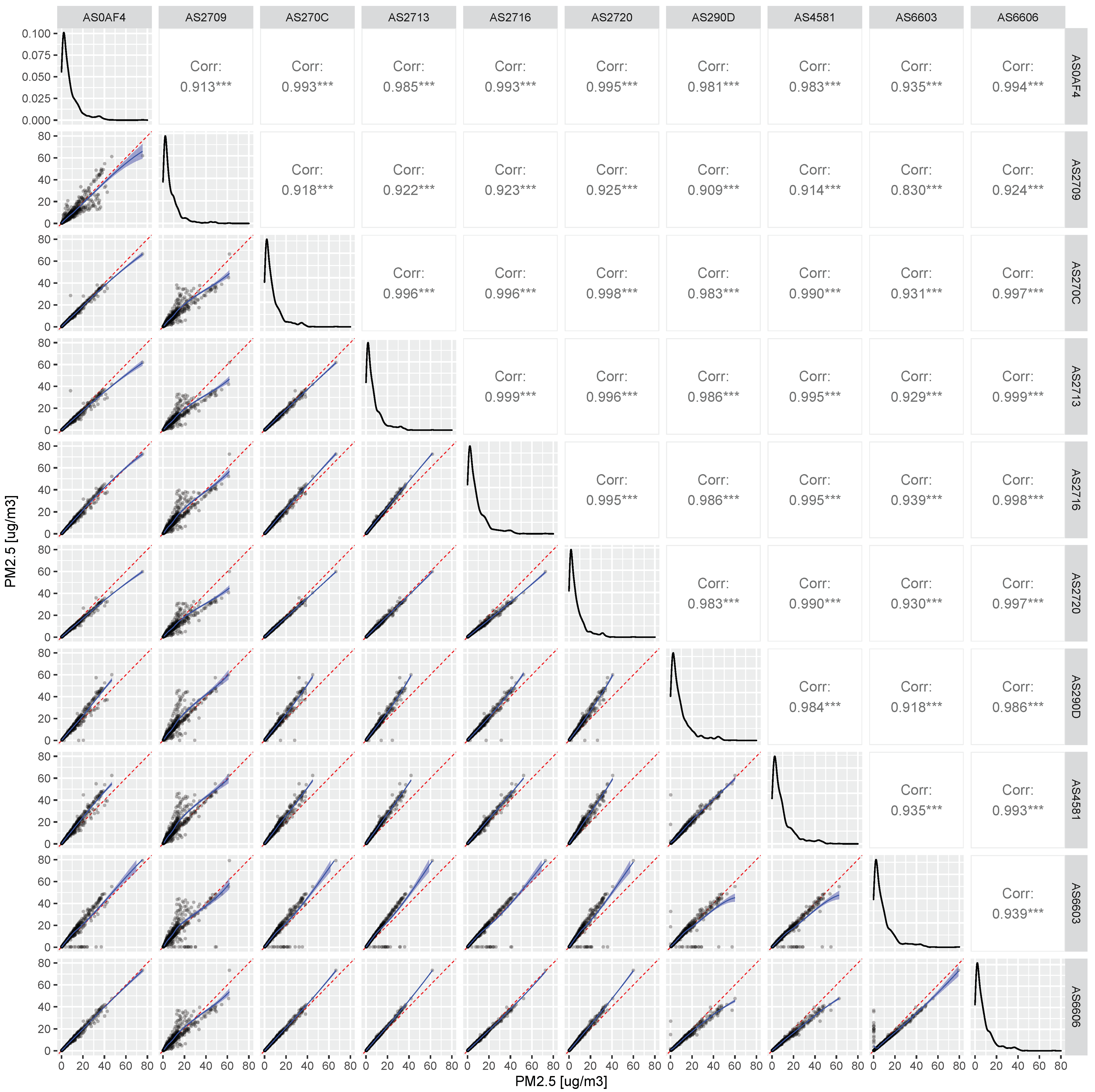
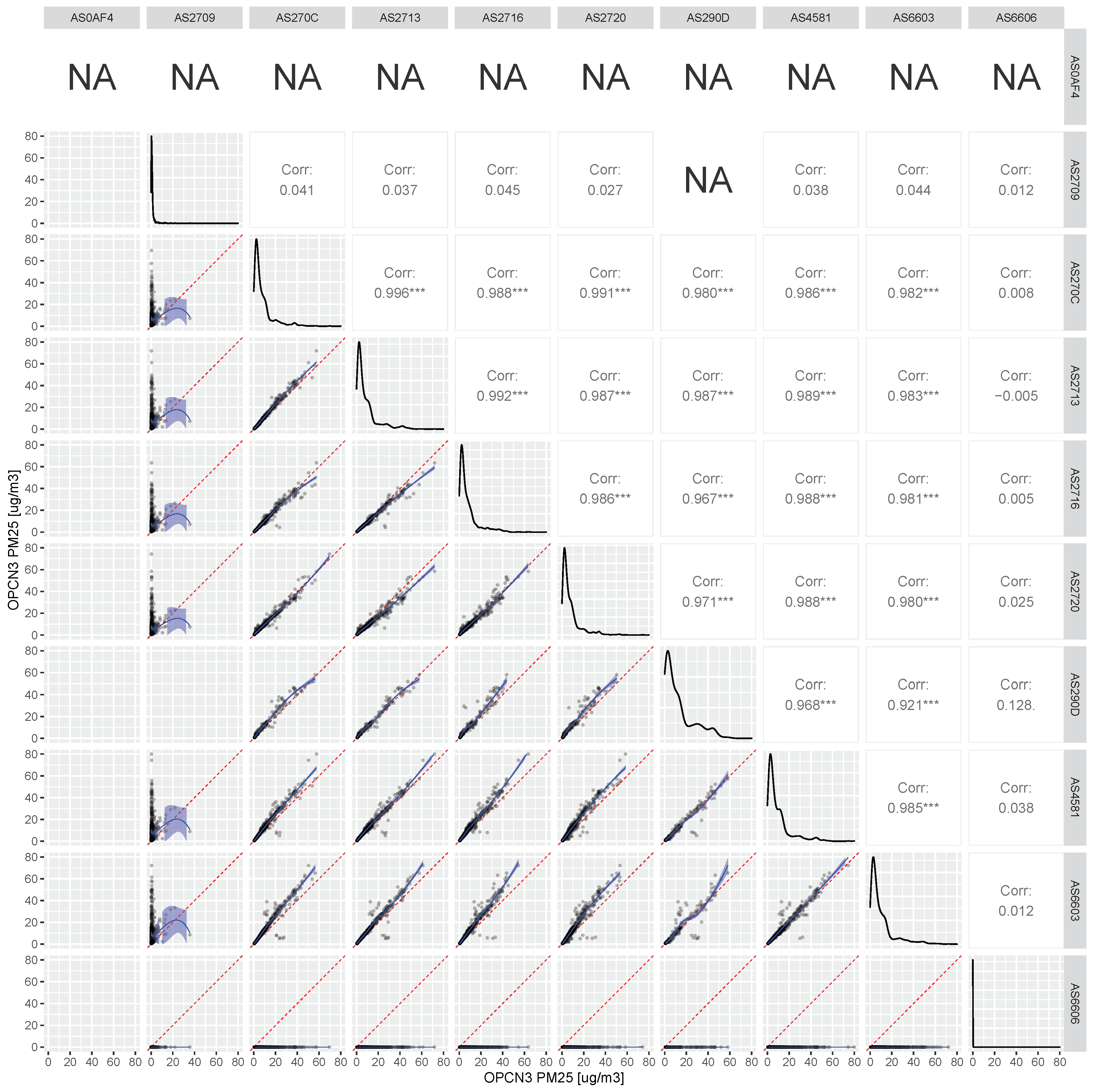
One of the first steps of the co-location study was to evaluate the consistency between individual sensors. This is important, because ideally any correction of the data, to improve the accuracy, should be valid for all sensors. Such an intercomparison between sensor readings can most easily be carried out using a scatterplot matrix. Figure 3 shows this for the factory-calibrated PM_2.5 readings of the OPC-N3 sensor. The inter-sensor comparison shows mostly reasonable results, with Pearson correlation (Corr) values consistently over 0.9. The unit AS2709 shows considerably more scatter with respect to all the other units, so there is some suspicion of sensor malfunction for this particular unit.

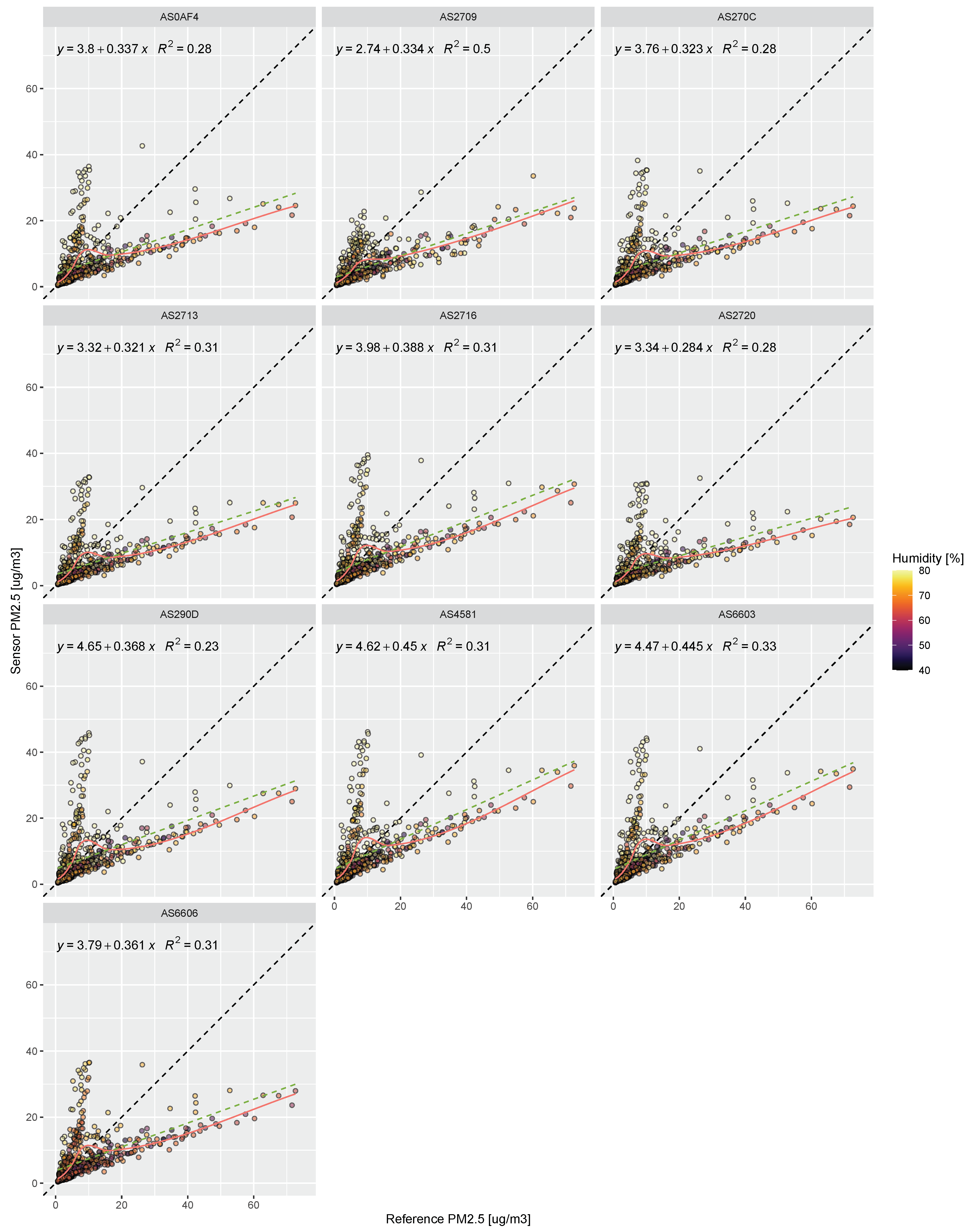
Figure 4 shows scatterplots directly comparing the factory-calibrated sensor PM_2.5 mass concentration against the reference PM_2.5 mass concentration at Schancheholen, during the co-location period. While all sensors appear to behave quite similarly overall, it is obvious that relative humidity significantly affects the sensor measurements, causing strong positive biases at very low true concentrations, around 5 to 10 $\mathsf{\mu }$g m${}^{-3}$. As this causes a split shape of the scatter cloud, the correlation between sensor observations and the reference instrument data is low, with Corr values ranging from 0.48 to 0.70, and the fitted R² value for all sensor units ranging from 0.25 to 0.5.

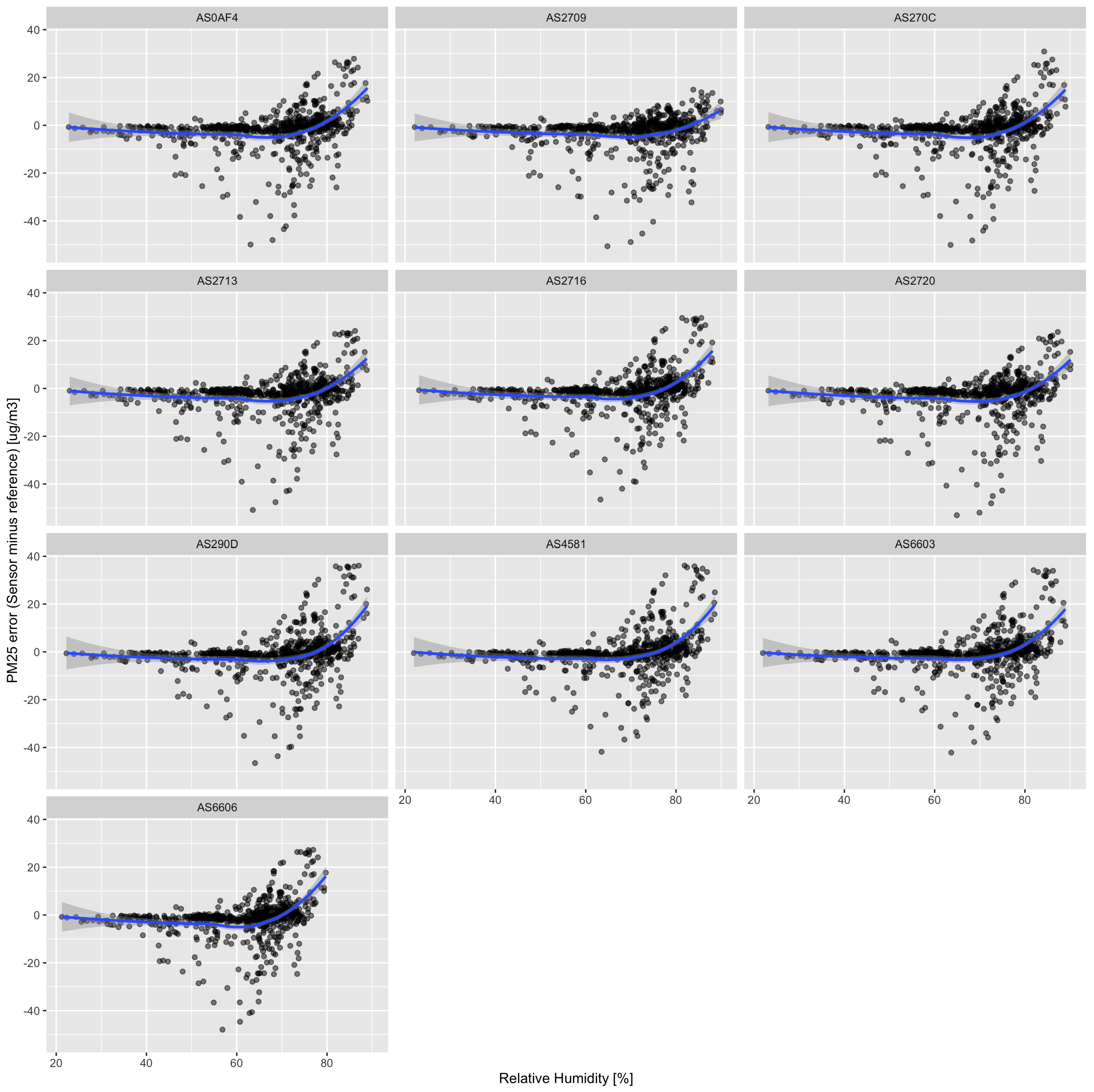
The error induced by humidity is further demonstrated in Figure 5, which shows the difference between the sensor PM_2.5 and the reference PM_2.5 as a function of relative humidity. It can be observed that, for humidity values of greater than 80%, the sensor clearly overestimates the true PM_2.5 concentration. However, negative outliers occur for all sensors, even for lower humidities, and thus likely have a different origin.

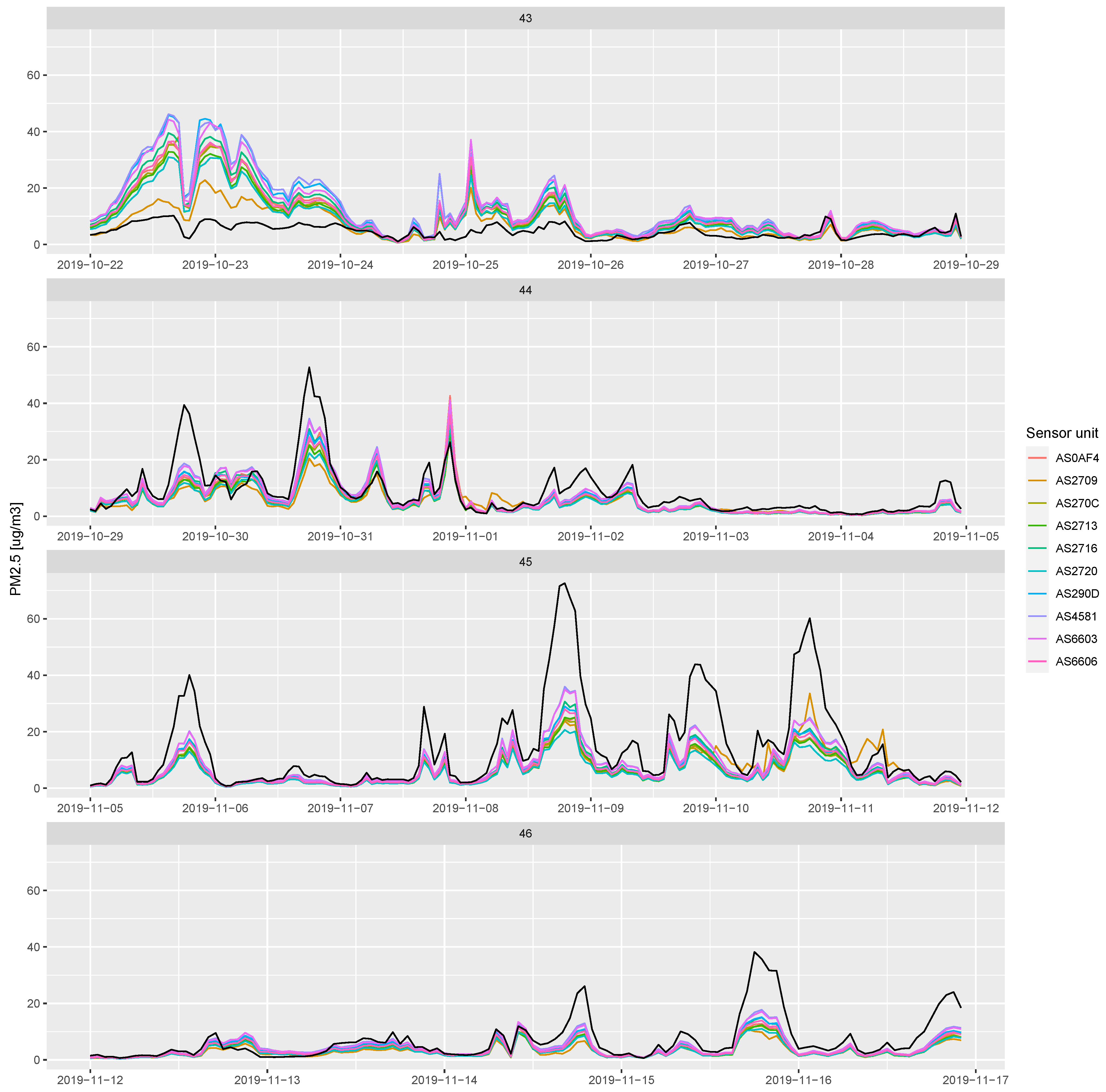
Figure 6 shows time series of the PM_2.5 measurements of all sensor units compared to the reference PM_2.5. It can be observed that, while the sensor signals generally follow the temporal patterns of the reference (i.e., they show peaks when the reference shows peaks), there are substantial temporally varying biases. For example, in week 43, the sensors typically overestimate the PM_2.5 mass concentrations compared to the reference, whereas in weeks 45/46, they generally underestimate the true mass concentrations.

A more in-depth analysis and discussion of the Alphasense OPC-N3 sensor performance under Norwegian environmental conditions, can be found in [4].

3.1.2. Evaluation of NO₂

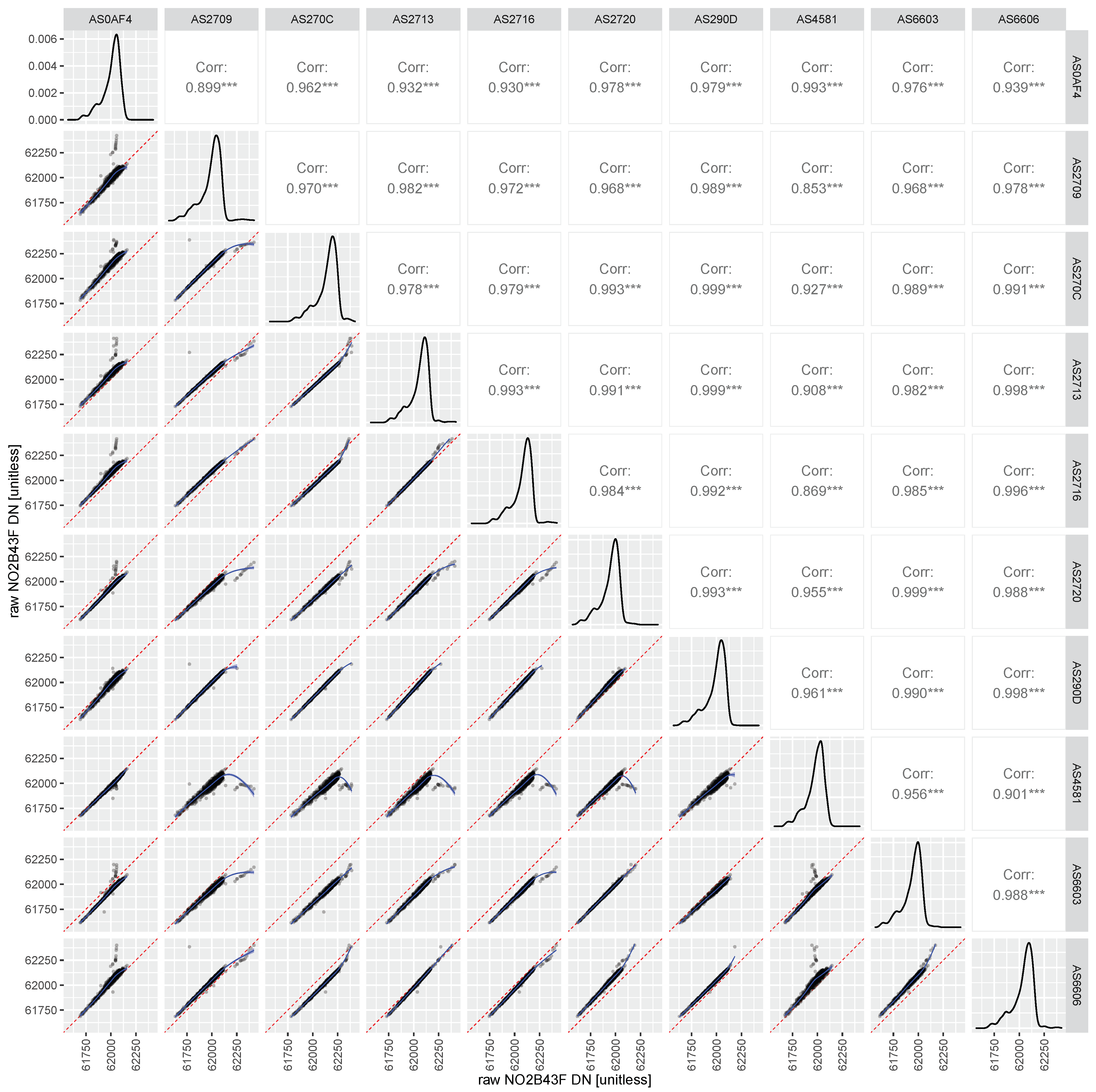
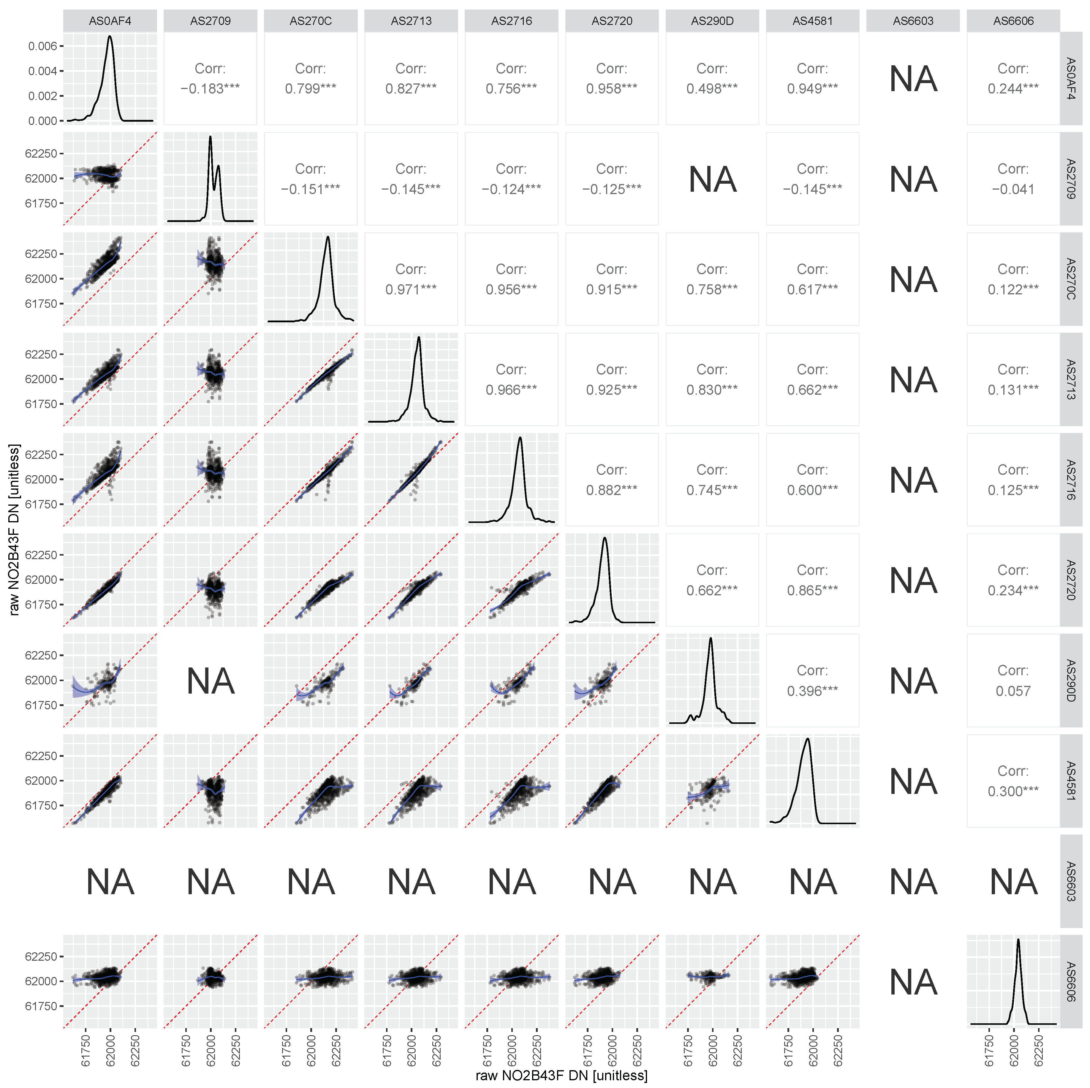
For the NO₂ sensors (Figure 7), the intercomparison scatterplots indicate a quite good agreement overall, with Corr values of consistently 0.9 or greater. Two aspects are noticeable: unit AS4581 shows significantly more scatter than the other sensor systems, and unit AS270C appears to have biases against several other units.

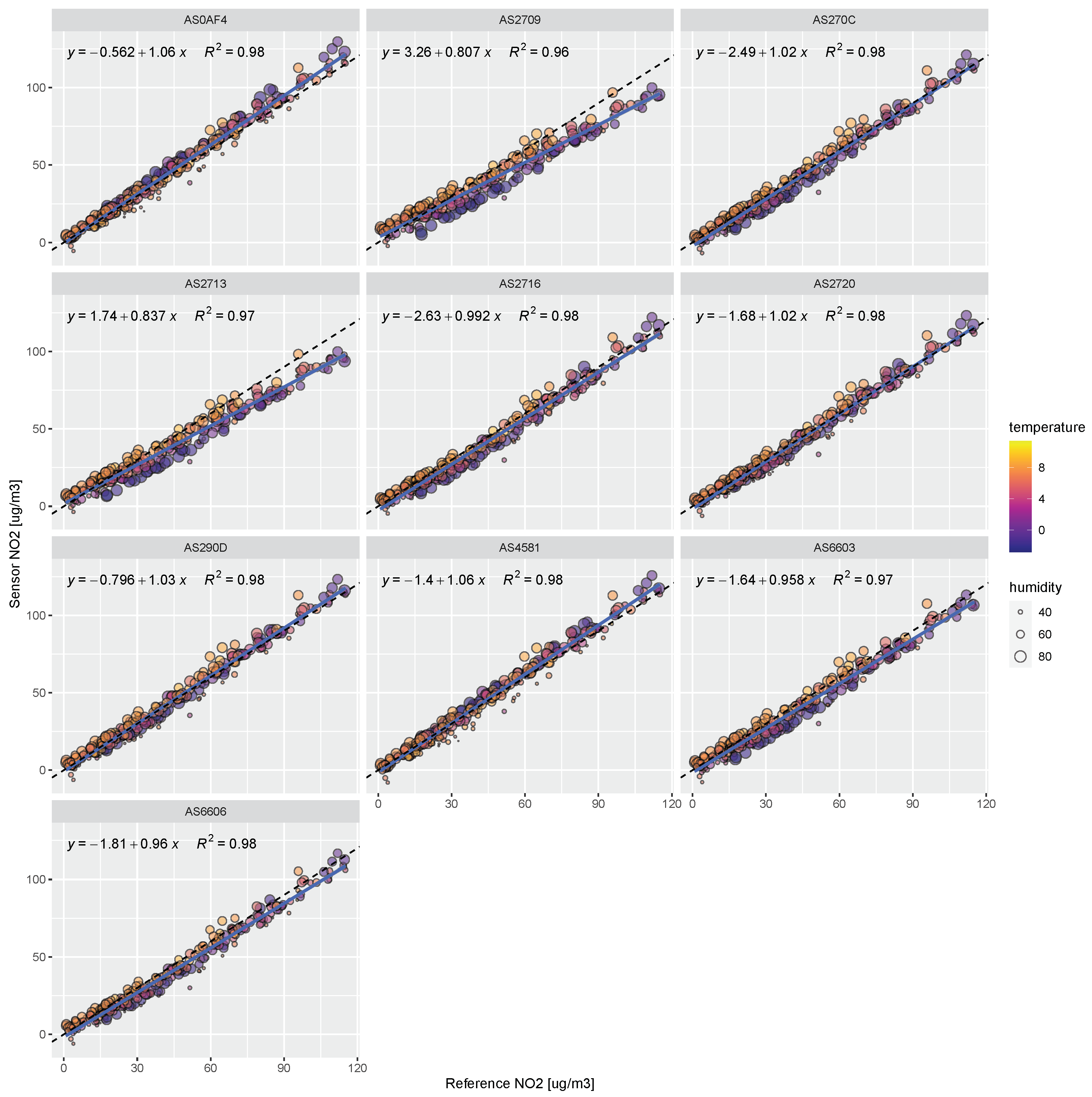
Figure 8 shows the time series for the test period, with the black line indicating the observations obtained by the reference analyzer and the red line showing the calibrated sensor NO₂. Overall, we can observe an excellent correspondence between the two datasets, for the relatively short test period. A slight underestimation is exhibited by units AS2709 and AS2713. The same data is shown in the form of scatterplots in Figure 9. The correlations are excellent for all ten units, with consistent Corr values ranging from 0.98 to 0.99, and fitted R² values of 0.96 and higher. With the exception of units AS2709 and AS2713, no significant biases are visible with respect to the 1:1 reference line.

However, it should be noted here that the testing period for which data is shown was only relatively short (ca. 2 weeks), and was following the training period, with very similar environmental conditions. As such, the calibration is expected to perform quite well, as it is an ideal scenario. It is likely that the obtainable sensor accuracy is significantly lower in substantially different environmental conditions, and this has been documented in several studies [5]. Even though temperature was included as a predictor variable in the calibration, a slight residual temperature dependence is still visible in the data, with lower temperatures resulting in slightly negative, and higher temperatures in slightly positive, biases (see Figure 9). This indicates that the treatment of temperature in the calibration equation was not optimal and that it would be worthwhile considering other calibration methods, to eliminate this residual sensitivity of the NO₂ signal on ambient temperature. It should be noted, however, that this sensitivity on temperature varies significantly from sensor unit to sensor unit: while, for example, units AS2709 and AS2713 show this effect quite prominently, it is nearly not noticeable in units AS2720 and AS290D.

Finally,

Table 3. Summary statistics of applying the sensor-specific multilinear regression models for NO₂ to the testing period. MB is the mean bias, MAE is the mean absolute error, and RMSE is the root mean squared error. R² is the coefficient of determination. All values given in units of $\mathsf{\mu }$g m${}^{-3}$ except R² (unitless).

Sensor ID	MB	MAE	RMSE	${\mathbf{R}}^2$
AS0AF4	1.96	3.78	5.01	0.98
AS2709	−4.81	7.15	8.99	0.96
AS270C	−1.70	3.55	4.70	0.98
AS2713	−5.09	6.69	8.48	0.97
AS2716	−2.98	4.32	5.46	0.98
AS2720	−0.83	3.04	4.12	0.98
AS290D	0.40	3.11	4.18	0.98
AS4581	0.94	3.53	4.68	0.98
AS6603	−3.40	4.72	5.92	0.97
AS6606	−3.50	4.57	5.75	0.98
Average	−1.90	4.45	5.73	0.98

gives the summary statistics of applying the multilinear regression model to each sensor system during the testing period. Based on the RMSE metric, unit AS2720 achieved the best result (with an RMSE of only 4.12 $\mathsf{\mu }$g m${}^{-3}$) and unit AS2709 the worst (with an RMSE of nearly 9 $\mathsf{\mu }$g m${}^{-3}$). Overall, the mean RMSE of all units was 5.73 $\mathsf{\mu }$g m${}^{-3}$.

3.2. Deployment

During the deployment phase, from 18 November 2019 to 25 May 2020, nine out of the ten sensor units were deployed at various locations, without access to observations from reference instrumentation. As such, no evaluation could be carried out for these units during the deployment period, however, the data provided by them can be exploited for various applications, including, for example, combination with model output (see Section 3.5). A single sensor unit (AS2713) remained at the Schancheholen reference site during the entire deployment period, and we use its data here to test how well the initial calibration, carried out in the month of November, performed during other periods, with substantially different environmental conditions.

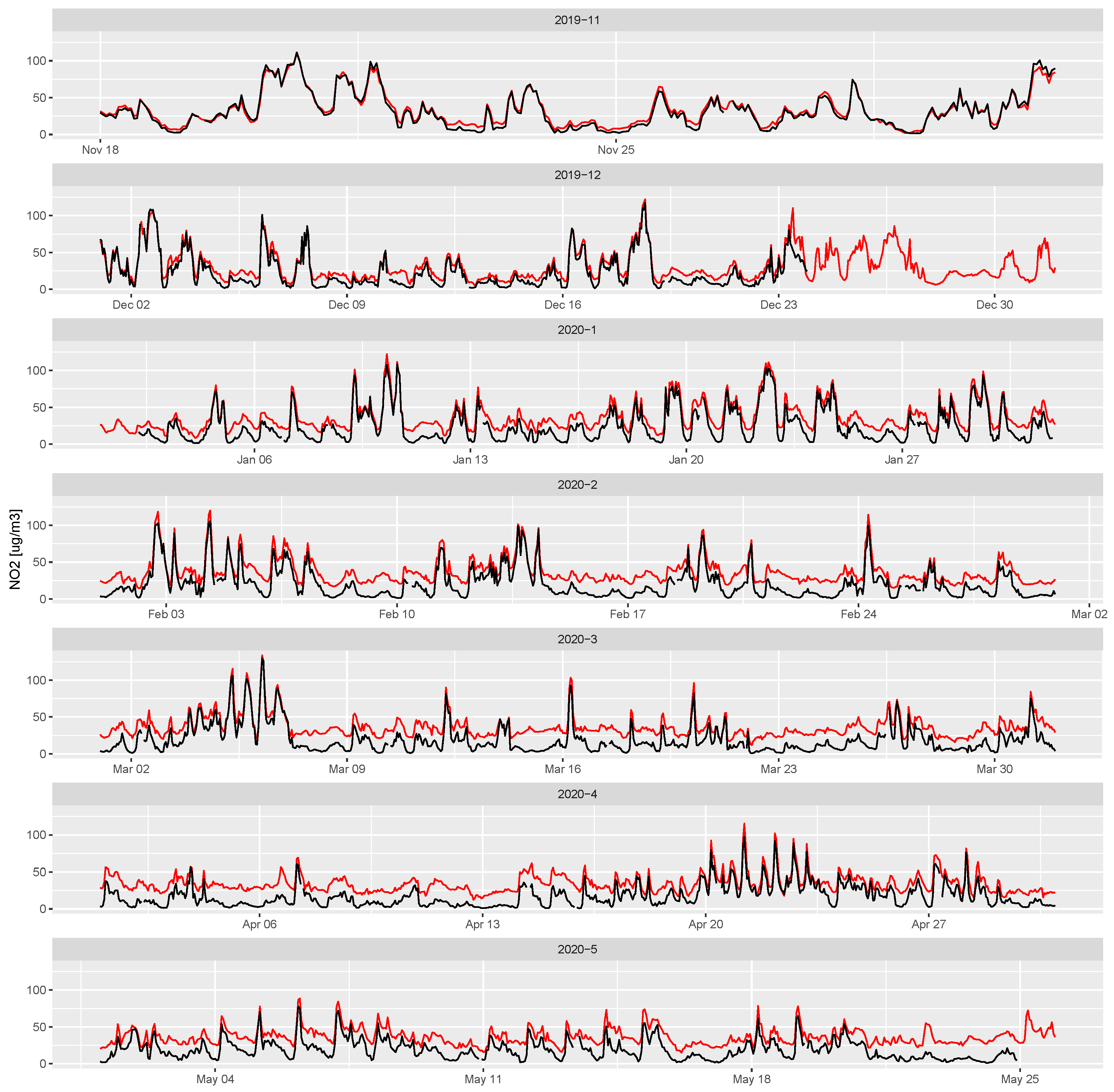
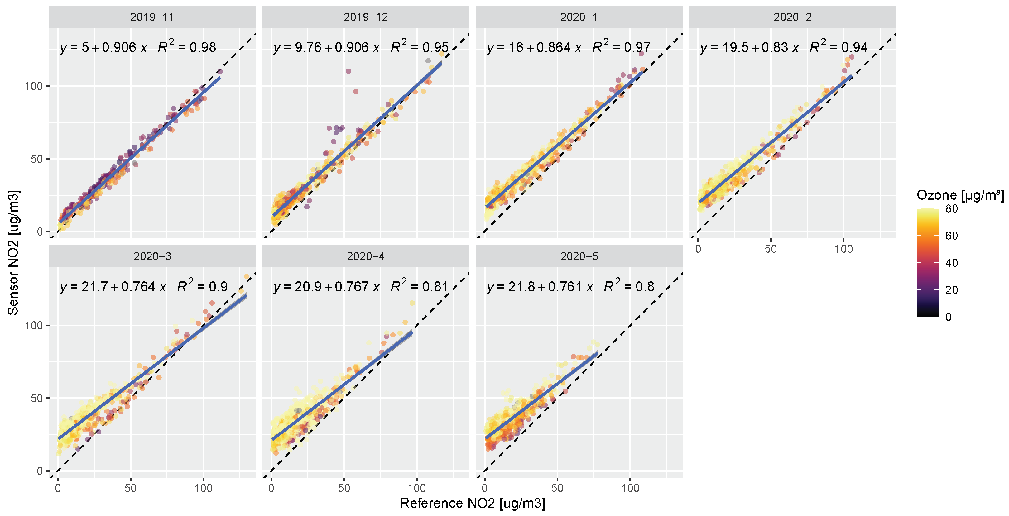
Figure 10 shows time series of the calibrated NO₂ signal from the AS2713 unit during the deployment period. We can see that, during the beginning of the deployment period (e.g., November and December 2019), the sensor signal matches that of the reference quite well. However, beginning in around January 2020, a consistent bias of approximately 20 $\mathsf{\mu }$g m${}^{-3}$ appears to develop, that stays mostly constant until the end of the deployment period.

This bias is likely caused by environmental conditions (primarily ozone concentration and temperature) that are substantially different compared to those that were present during the calibration period. In particular, the effect of ozone concentration can be seen very well in Figure 11. The bias at lower NO₂ concentrations is obvious, particularly for the later months, and is to some extent correlated with an increase in ozone during this period. Nonetheless, despite the substantial biases found in the later parts of the deployment period, Figure 11 also indicates that the correlation between sensor NO₂ and reference NO₂ remains quite good, with R² levels of 0.80 to 0.98 and Corr2 values ranging from 0.90 to 0.99. If the described biases cannot be adequately compensated for as part of the calibration, other methods exist to postprocess the data accordingly, e.g., regular bias correction of all sensors using the mean NO₂ concentration of one or more air quality reference stations, when the NO₂ concentration field can be assumed to be highly homogeneous in space [23,57,58].

3.3. Post-Deployment Co-Location

A second co-location of the ten sensor systems was carried out after the end of the deployment period. On 25 May 2020, all the units were again mounted at the Schancheholen air quality monitoring station, in order to test to what extent the behavior of the individual sensors had changed over time. Post-deployment data for this study was available until 5 July 2020. Figure 12 and Figure 13 show scatterplot matrices of the sensor-provided PM_2.5 and NO₂ signals of all ten sensor units during the post-deployment co-location period. In both cases, there is one sensor system that consistently did not provide any data at all during the post-deployment co-location period: for PM_2.5 this was the OPC-N3 sensor in the AS0AF4 unit, whereas for NO₂ it was the NO2B43F sensor in the AS6603 unit.

We can compare these figures directly to Figure 3 and Figure 7, respectively. We can see that sensor-to-sensor consistency has deteriorated slightly for PM_2.5. Whereas before only AS2709 showed a somewhat questionable signal, now it is also units AS6606 that exhibit erratic behavior compared to all the other units. The rest of the units show roughly similar sensor-to-sensor correspondence, as in the pre-deployment co-location, with Corr values typically over 0.95.

When we compare Figure 13 against the results from the pre-deployment co-location (Figure 7), we can observe a substantial decrease in the inter-sensor correspondence, that can likely be attributed to the deterioration of the electrochemical sensors during the deployment period. The NO2_B43F sensor in the AS6603 did not provide data during the post-deployment co-location period. In most of the other pairings, the correlation has decreased substantially, from values of mostly consistently over 0.9 in the pre-deployment co-location, to a wide range of between 0.2 and 0.9, with most pairings in the 0.8 range. Some sensors, such as the ones in AS2709 and AS6606, have completely lost any correspondence with the signal from the sensors in the other units.

3.4. Results of Humidity Correction for PM

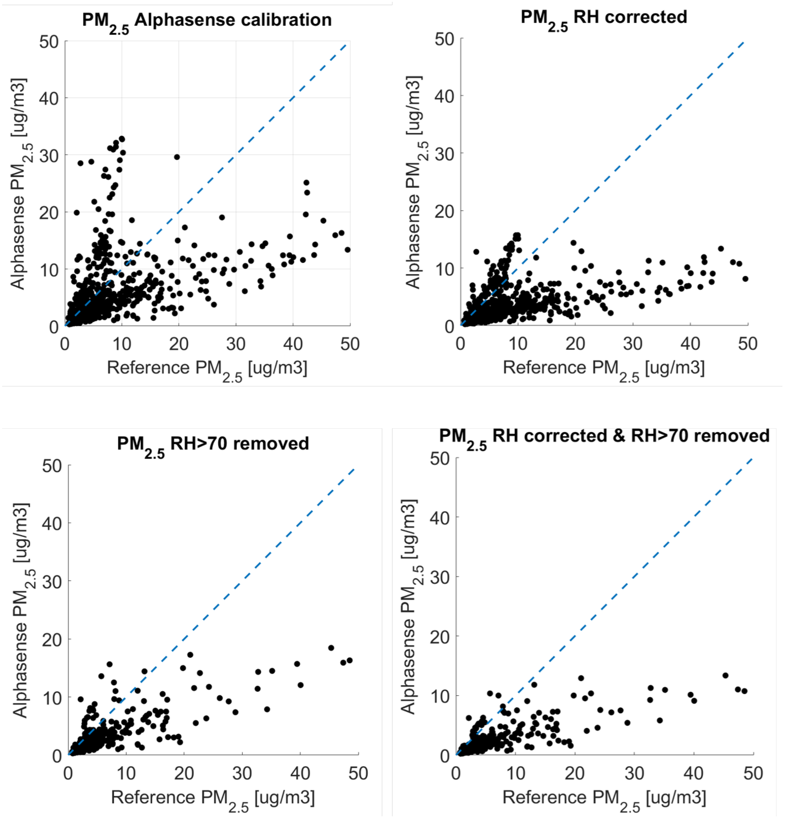
As seen in Figure 4 and Figure 5, humidity significantly affects the sensor measurements. Therefore, we implemented three types of corrections, which are shown in Figure 14 for sensor unit AS2713 as a representative example. The first correction method was to account for relative humidity according to [33], the second method was removing data points where the relative humidity was greater than 70 percent, and the third one was a combination of both of these methods.

The results are shown as summary statistics in

Table 4. Summary statistics of manufacturer-calibrated PM_2.5 mass concentrations against the reference data, during the co-location. RMSE is the root mean squared error and MAD is the mean absolute deviation.

Sensor Unit	Bias	Std. Dev.	RMSE	MAD	Intercept	Slope	R2
AS0AF4	−2.04	9.5	9.69	2.54	4.09	0.3	0.22
AS2709	−3.12	8.31	8.86	2.19	2.99	0.3	0.41
AS270C	−2.20	9.45	9.693	2.46	4.05	0.28	0.22
AS2713	−2.66	9.24	9.61	2.61	3.6	0.28	0.25
AS2720	−2.97	9.4	9.85	2.50	3.62	0.25	0.22
AS290D	−0.92	10.31	10.34	2.61	5.01	0.32	0.18
AS4581	−0.23	9.77	9.77	2.46	5.01	0.4	0.25
AS6603	−0.41	9.49	9.49	2.46	4.87	0.4	0.27
AS6606	−1.85	9.30	9.48	2.452	4.12	0.32	0.25
AS2716	−1.41	9.41	9.5	2.59	4.33	0.35	0.25
Average	−1.78	9.42	9.63	2.49	4.17	0.32	0.25

,

Table 5. Summary statistics of manufacturer-calibrated PM_2.5 mass concentrations against the reference data, during the co-location, after correction for relative humidity effects using Köhler theory. RMSE is the root mean squared error and MAD is the mean absolute deviation.

Sensor Unit	Bias	Std. Dev.	RMSE	MAD	Intercept	Slope	R2
AS0AF4	−4.82	9.08	10.28	2.42	2.34	0.19	0.32
AS2709	−5.45	8.89	10.41	2.36	1.73	0.18	0.49
AS270C	−4.91	9.138	10.36	2.37	2.31	0.18	0.32
AS2713	−5.19	9.09	10.46	2.63	2.04	0.18	0.35
AS2720	−5.47	9.31	10.79	2.56	2.00	0.15	0.32
AS290D	−4.21	9.23	10.11	2.56	2.85	0.2	0.26
AS4581	−3.75	8.76	9.52	2.35	2.87	0.25	0.34
AS6603	−3.86	8.719	9.52	2.35	2.78	0.25	0.36
AS6606	−4.09	8.93	9.82	2.4	2.73	0.23	0.31
AS2716	−4.444	8.86	9.91	2.39	2.46	0.22	0.35
Average	−4.62	9.00	10.12	2.44	2.41	0.20	0.34

,

Table 6. Summary statistics of manufacturer-calibrated PM_2.5 mass concentrations against the reference data, during the co-location, after removing observations with a relative humidity greater than 70 percent. RMSE is the root mean squared error and MAD is the mean absolute deviation.

Sensor Unit	Bias	Std. Dev.	RMSE	MAD	Intercept	Slope	R2
AS0AF4	−3.2	6.44	7.19	1.85	1.57	0.35	0.63
AS2709	−3.28	6.22	7.02	1.64	1.3	0.36	0.67
AS270C	−3.15	6.47	7.18	1.8	1.63	0.35	0.63
AS2713	−3.54	6.48	7.37	2.04	1.31	0.34	0.65
AS2720	−3.7	6.66	7.61	1.9	1.29	0.31	0.66
AS290D	−2.48	6.13	6.61	1.6	1.81	0.4	0.6
AS4581	−2.06	5.66	6.02	1.37	1.72	0.48	0.67
AS6603	−2.02	5.75	6.08	1.37	1.8	0.48	0.66
AS6606	−3.25	8.61	9.19	2.202	2.94	0.31	0.42
AS2716	−2.76	6.04	6.63	1.72	1.55	0.41	0.66
Average	−2.94	6.45	7.09	1.75	1.69	0.38	0.63

and

Table 7. Summary statistics of manufacturer-calibrated PM_2.5 mass concentrations against the reference data, during the co-location, after correction for relative humidity effects using Köhler theory, and after removing observations with a relative humidity greater than 70 percent. RMSE is the root mean squared error and MAD is the mean absolute deviation.

Sensor Unit	Bias	Std. Dev.	RMSE	MAD	Intercept	Slope	R2
AS0AF4	−4.23	7.11	8.26	2.08	1.26	0.25	0.61
AS2709	−4.24	6.97	8.15	2.1	1.11	0.25	0.64
AS270C	−4.2	7.15	8.27	2.02	1.31	0.25	0.61
AS2713	−4.5	7.17	8.44	2.25	1.07	0.24	0.64
AS2720	−4.57	7.34	8.63	2.22	1.07	0.22	0.62
AS290D	−3.64	6.78	7.69	1.93	1.47	0.28	0.59
AS4581	−3.36	6.44	7.25	1.86	1.43	0.34	0.66
AS6603	−3.35	6.52	7.32	1.83	1.5	0.34	0.65
AS6606	−4.82	9.02	10.23	2.38	2.15	0.22	0.44
AS2716	−3.92	6.78	7.82	2	1.25	0.28	0.65
Average	−4.08	7.13	8.21	2.07	1.36	0.27	0.61

. Overall, the Corr values increased substantially, from 0.25 to 0.65. The relative humidity correction according to [33] showed a very small improvement compared to the manufacturer calibration, in terms of correlation. The average correlation coefficient for the ten sensors increased from 0.25 to 0.34, however, the slope decreased on average from 0.32 to 0.2, and the RMSE increased on average from 9.6 to 10.1. The highest Corr values were found for the removal of data for relative humidity values over 70 percent, which resulted in an increase in average Corr values from 0.25 to 0.62. Due to the filtering, the average RMSE decreased to 7.1, and the slope increased to 0.38, suggesting that the sensor is not operating in a functioning condition when the relative humidity is over 70 percent. The removal of observations with relative humidity values greater than 70 percent was based on previous projects with other low cost sensor units, where the manufacturer defined the range of operation up to 70 percent relative humidity (for example [7]). Alphasense defines in their technical specifications of the OPC-N3 (http://www.alphasense.com/WEB1213/wp-content/uploads/2019/03/OPC-N3.pdf, accessed on 22 December 2022), an operational range of the sensor of up to 95 percent relative humidity, which seems to be unrealistic based on the results shown here, at least for Norwegian conditions.

The final correction seen in Table 7, shows the results of combining both methods (removing observations with humidity values greater than 70 percent and correction for relative humidity using Köhler theory). This correction did not further improve the statistics compared to just filtering the data for humidity values greater than 70 percent.

3.5. High-Resolution Mapping through Data Assimilation

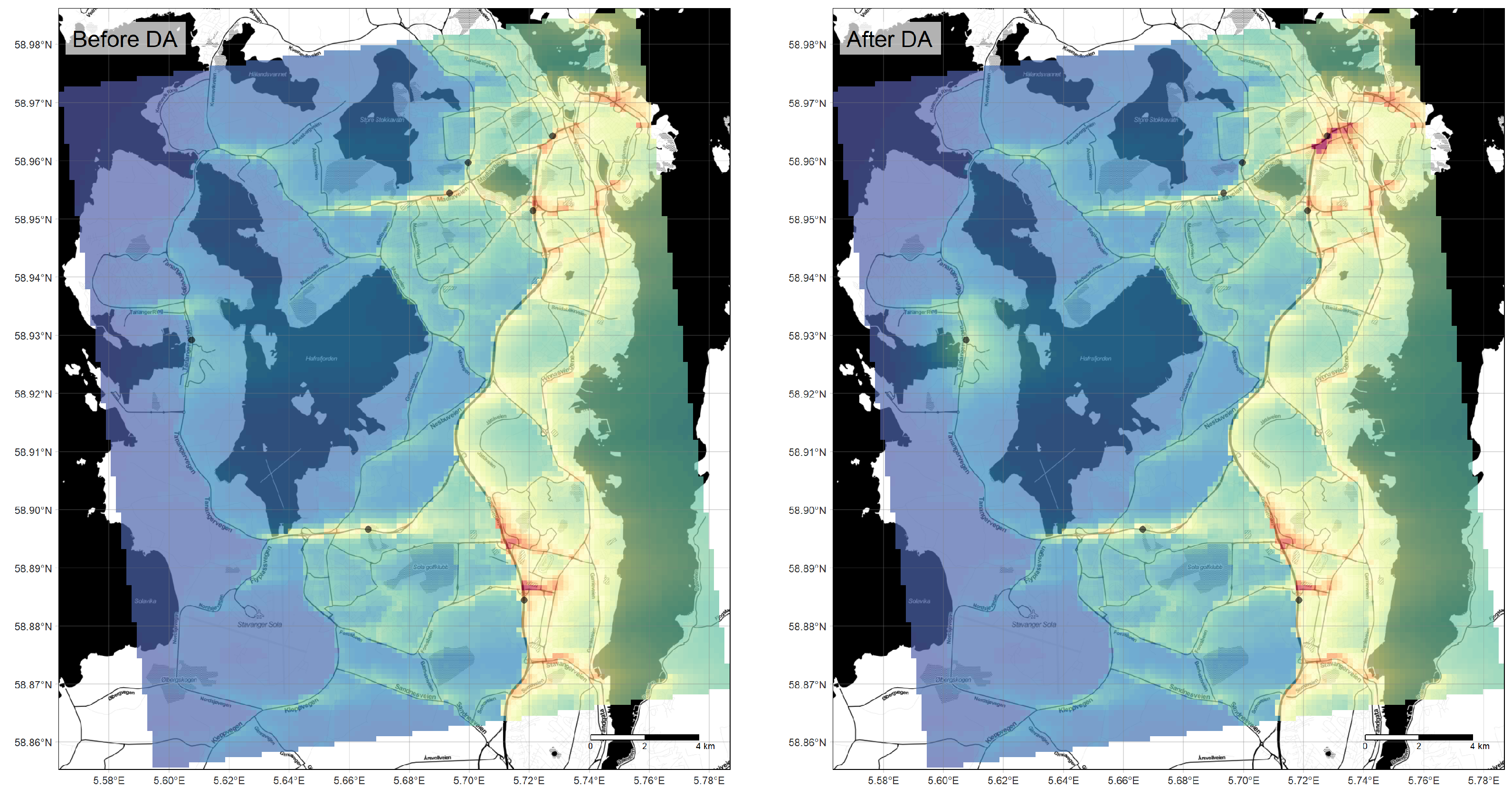
A short example on the use of simple data assimilation techniques for exploiting the observations from small low-cost sensor networks is given in the following. Figure 15 and Figure 16 show an illustration of how the results of the data assimilation process can look in principle, even for a very small sensor network, as available in this study. Figure 15 shows the available input data of NO₂ concentration for one arbitrary hour (9 January 2020 at 15 UTC), for the greater Stavanger area. Some differences between the model forecast, here from the uEMEP model [55,56], and the sensor observations are obvious, and the innovation, i.e., the difference between these two datasets, is being used to update the model forecast. Alternatively, one can think of the process as the point-based observations being interpolated in space, using the spatial field from the model as a guide. Figure 16 shows the output of the data assimilation process, namely the original model datasets (left panel) compared to the analysis resulting from assimilation of the sensor observations (right panel). While the differences are subtle, it can be seen that, for example, the downtown area of Stavanger shows increased concentration levels based on the sensor observations made there. Similarly, for the area around the sensor system located in the very western side of the domain, the analysis shows slightly elevated NO₂ concentration values. For all other sites, the model forecast has been slightly reduced according to the innovation data shown in Figure 15 (right panel).

4. Conclusions and Recommendations

A small network of air quality sensor systems was set up in the region of Stavanger, Norway, with the main goal of evaluating its performance and operation under challenging Nordic winter conditions. A total number of ten AirSensEUR units were first co-located at an air quality monitoring station equipped with reference instrumentation. This was done for evaluating the performance of the PM_2.5 sensors against the reference, and in the case of NO₂ in order to both evaluate the sensors, and to calibrate them, i.e., to allow for a conversion of the raw measurement units into physical concentration units of $\mathsf{\mu }$g m${}^{-3}$. Subsequently, nine of the ten systems were deployed at various roadside locations, of which seven were further considered in this study. After deployment, the sensor systems were again co-located at the air quality monitoring station for evaluating possible deterioration of the sensors.

The results of the co-location indicate, for NO₂, a very good agreement with the reference (with consistent Corr values of around 0.98), in the weeks immediately after the calibration period. However, the calibration is sensitive to the environmental conditions. As such, significant changes in the environmental conditions (e.g., temperature and ozone concentrations) can negatively affect the calibration over the long term and result in significant biases.

Ideally the training period for the calibration should encompass the entire range of environmental conditions that is to be expected later on during the deployment. This is, however, not always feasible in practice, as it would typically mean several months of co-location period. Alternatively, there are relatively easy methods for eliminating such biases in post-processing, for example for NO₂, by regularly resetting all sensors to the station-based average concentrations during a period in which the spatial patterns of NO₂ within a city are most homogeneous (for example at around 03:00 at night). Such approaches have been used previously, for example by [23,57], or [58]. Another possibility is a lab-calibration in a climate chamber, where all potential cross-sensitivites and environmental effects could be simulated relatively quickly for a single sensor [11,59], and the resulting calibration could subsequently be applied to the remaining sensors, assuming that they all behave identically, which is mostly, but not entirely, the case considering the results shown in Figure 9. If this is carried out in a very comprehensive manner, it has the potential for resulting in sensor calibrations that are robust in the majority of environmental conditions that might be encountered in the field. However, such a process typically is prohibitively expensive. It should also be noted that, the inter-sensor consistency of the used electrochemical sensors decreased substantially over the six-month deployment period, thus further complicating possible correction schemes over time.

For PM_2.5 from the OPC-N3 sensor, the results of the co-location showed a relatively poor agreement with the reference data, when using the factory-calibrated output. An attempt was made to increase the performance using a correction algorithm based on Köhler theory, which did not substantially improve the statistics. Restricting the data to observations with relative humidity values of less than 70 percent resulted in improvements in data accuracy, with reasonable R² values, of about 0.65. This indicates that when the OPC-N3 devices are being used at high relative humidity, they are being used outside of the measurement range that can be realistically expected to provide reasonable values, according to the underlying physical measurement principle. However, filtering for observations made under high relative humidity leads to a substantial loss in data coverage (decrease in temporal coverage of 61% and 31% during the deployment period for an RH threshold of 70% and 80%, respectively).

Finally, a brief illustration was given of the use of a data assimilation scheme for exploiting the observations from a relatively small network of low-cost sensors. When combined with high-resolution output of an air quality model, data assimilation can add value to the observations, by interpolating between them in a mathematically objective fashion, and at the same time add value to the model, by correcting it with actual observations. As a result, we find that the data assimilation process is able to provide maps of air quality with realistic spatial patterns, even for relatively small sensor networks, as the one available here.

Overall, the comparatively small network of AirSensEUR systems was found to be generally useful for providing additional information on NO₂ and PM_2.5 beyond what the air quality monitoring stations routinely provide, particularly for providing additional indicative information about urban-scale spatial patterns, for which the regulatory monitoring network is typically not dense enough. However, we saw indications that the challenging Nordic winter conditions negatively impact the lifetime of the electrochemical cells. In addition, the required routines for co-location, calibration, and post-processing for operating a sensor network are associated with significant labor, and users have to individually weigh this expense against the additional information obtained from the network. Future work should focus on automated algorithms for network calibration of the devices, without the need for expensive co-location exercises.

References

- Snyder, E.G.; Watkins, T.H.; Solomon, P.A.; Thoma, E.D.; Williams, R.W.; Hagler, G.S.W.; Shelow, D.; Hindin, D.A.; Kilaru, V.J.; Preuss, P.W. The Changing Paradigm of Air Pollution Monitoring. Environ. Sci. Technol. 2013, 47, 11369–11377. [Google Scholar] [CrossRef]
- Karagulian, F.; Barbiere, M.; Kotsev, A.; Spinelle, L.; Gerboles, M.; Lagler, F.; Redon, N.; Crunaire, S.; Borowiak, A. Review of the Performance of Low-Cost Sensors for Air Quality Monitoring. Atmosphere 2019, 10, 506. [Google Scholar] [CrossRef] [Green Version]
- WMO. An Update on Low-Cost Sensors for the Measurement of Atmospheric Composition; Technical Report WMO Report 1215; World Meteorological Organization (WMO): Geneva, Switzerland, 2021. [Google Scholar]
- Vogt, M.; Schneider, P.; Castell, N.; Hamer, P. Assessment of Low-Cost Particulate Matter Sensor Systems against Optical and Gravimetric Methods in a Field Co-Location in Norway. Atmosphere 2021, 12, 961. [Google Scholar] [CrossRef]
- Kang, Y.; Aye, L.; Ngo, T.D.; Zhou, J. Performance evaluation of low-cost air quality sensors: A review. Sci. Total Environ. 2022, 818, 151769. [Google Scholar] [CrossRef] [PubMed]
- CEN/TS 17660-1:2021; Air Quality—Performance Evaluation of Air Quality Sensor Systems—Part 1: Gaseous Pollutants in Ambient Air. European Committee for Standardization (CEN): Brussels, Belgium, 2021.
- Liu, H.Y.; Schneider, P.; Haugen, R.; Vogt, M. Performance assessment of a low-cost PM2. 5 sensor for a near four-month period in Oslo, Norway. Atmosphere 2019, 10, 41. [Google Scholar] [CrossRef] [Green Version]
- Schneider, P.; Bartonova, A.; Castell, N.; Dauge, F.R.; Gerboles, M.; Hagler, G.S.; Hüglin, C.; Jones, R.L.; Khan, S.; Lewis, A.C.; et al. Toward a Unified Terminology of Processing Levels for Low-Cost Air-Quality Sensors. Environ. Sci. Technol. 2019, 53, 8485–8487. [Google Scholar] [CrossRef] [Green Version]
- Spinelle, L.; Gerboles, M.; Villani, M.G.; Aleixandre, M.; Bonavitacola, F. Field calibration of a cluster of low-cost available sensors for air quality monitoring. Part A: Ozone and nitrogen dioxide. Sens. Actuators B Chem. 2015, 215, 249–257. [Google Scholar] [CrossRef]
- Spinelle, L.; Gerboles, M.; Villani, M.G.; Aleixandre, M.; Bonavitacola, F. Field calibration of a cluster of low-cost commercially available sensors for air quality monitoring. Part B: NO, CO and CO2. Sens. Actuators B Chem. 2017, 238, 706–715. [Google Scholar] [CrossRef]
- Castell, N.; Dauge, F.R.; Schneider, P.; Vogt, M.; Lerner, U.; Fishbain, B.; Broday, D.; Bartonova, A. Can commercial low-cost sensor platforms contribute to air quality monitoring and exposure estimates? Environ. Int. 2017, 99, 293–302. [Google Scholar] [CrossRef] [PubMed]
- Castell, N.; Schneider, P.; Grossberndt, S.; Fredriksen, M.F.; Sousa-Santos, G.; Vogt, M.; Bartonova, A. Localized real-time information on outdoor air quality at kindergartens in Oslo, Norway using low-cost sensor nodes. Environ. Res. 2018, 165, 410–419. [Google Scholar] [CrossRef]
- Schneider, P.; Castell, N.; Dauge, F.R.; Vogt, M.; Lahoz, W.A.; Bartonova, A. A Network of Low-Cost Air Quality Sensors and Its Use for Mapping Urban Air Quality. In Mobile Information Systems Leveraging Volunteered Geographic Information for Earth Observation; Bordogna, G., Carrara, P., Eds.; Earth Systems Data and Models; Springer International Publishing: Cham, Switzerland, 2018; pp. 93–110. [Google Scholar]
- Castell, N.; Kobernus, M.; Liu, H.Y.; Schneider, P.; Lahoz, W.; Berre, A.J.; Noll, J. Mobile technologies and services for environmental monitoring: The Citi-Sense-MOB approach. Urban Clim. 2015, 14, 370–382. [Google Scholar] [CrossRef]
- Popoola, O.A.M.; Carruthers, D.; Lad, C.; Bright, V.B.; Mead, M.I.; Stettler, M.E.J.; Saffell, J.R.; Jones, R.L. Use of networks of low cost air quality sensors to quantify air quality in urban settings. Atmos. Environ. 2018, 194, 58–70. [Google Scholar] [CrossRef]
- Morawska, L.; Thai, P.K.; Liu, X.; Asumadu-Sakyi, A.; Ayoko, G.; Bartonova, A.; Bedini, A.; Chai, F.; Christensen, B.; Dunbabin, M.; et al. Applications of low-cost sensing technologies for air quality monitoring and exposure assessment: How far have they gone? Environ. Int. 2018, 116, 286–299. [Google Scholar] [CrossRef] [PubMed]
- Yatkin, S.; Gerboles, M.; Borowiak, A.; Davila, S.; Spinelle, L.; Bartonova, A.; Dauge, F.; Schneider, P.; Van Poppel, M.; Peters, J.; et al. Modified Target Diagram to check compliance of low-cost sensors with the Data Quality Objectives of the European air quality directive. Atmos. Environ. 2022, 273, 118967. [Google Scholar] [CrossRef]
- Hagler, G.S.W.; Williams, R.; Papapostolou, V.; Polidori, A. Air Quality Sensors and Data Adjustment Algorithms: When Is It No Longer a Measurement? Environ. Sci. Technol. 2018, 52, 5530–5531. [Google Scholar] [CrossRef] [Green Version]
- Walker, S.E.; Solberg, S.; Schneider, P.; Guerreiro, C. The AirGAM 2022r1 air quality trend and prediction model. Geosci. Model Dev. 2023, 16, 573–595. [Google Scholar] [CrossRef]
- Levy Zamora, M.; Buehler, C.; Lei, H.; Datta, A.; Xiong, F.; Gentner, D.R.; Koehler, K. Evaluating the Performance of Using Low-Cost Sensors to Calibrate for Cross-Sensitivities in a Multipollutant Network. ACS EST Eng. 2022, 2, 780–793. [Google Scholar] [CrossRef] [PubMed]
- Ionascu, M.E.; Castell, N.; Boncalo, O.; Schneider, P.; Darie, M.; Marcu, M. Calibration of CO, NO2, and O3 Using Airify: A Low-Cost Sensor Cluster for Air Quality Monitoring. Sensors 2021, 21, 7977. [Google Scholar] [CrossRef] [PubMed]
- Malings, C.; Tanzer, R.; Hauryliuk, A.; Kumar, S.P.; Zimmerman, N.; Kara, L.B.; Presto, A.A.; Subramanian, R. Development of a general calibration model and long-term performance evaluation of low-cost sensors for air pollutant gas monitoring. Atmos. Meas. Tech. 2019, 12, 903–920. [Google Scholar] [CrossRef] [Green Version]
- Van Zoest, V.; Osei, F.B.; Stein, A.; Hoek, G. Calibration of low-cost NO2 sensors in an urban air quality network. Atmos. Environ. 2019, 210, 66–75. [Google Scholar] [CrossRef]
- Zuidema, C.; Schumacher, C.S.; Austin, E.; Carvlin, G.; Larson, T.V.; Spalt, E.W.; Zusman, M.; Gassett, A.J.; Seto, E.; Kaufman, J.D. Deployment, Calibration, and Cross-Validation of Low-Cost Electrochemical Sensors for Carbon Monoxide, Nitrogen Oxides, and Ozone for an Epidemiological Study. Sensors 2021, 21, 4214. [Google Scholar] [CrossRef]
- Feenstra, B.; Papapostolou, V.; Hasheminassab, S.; Zhang, H.; Der Boghossian, B.; Cocker, D.; Polidori, A. Performance evaluation of twelve low-cost PM2. 5 sensors at an ambient air monitoring site. Atmos. Environ. 2019, 216, 116946. [Google Scholar] [CrossRef]
- Cavaliere, A.; Carotenuto, F.; Di Gennaro, F.; Gioli, B.; Gualtieri, G.; Martelli, F.; Matese, A.; Toscano, P.; Vagnoli, C.; Zaldei, A. Development of low-cost air quality stations for next generation monitoring networks: Calibration and validation of PM2. 5 and PM10 sensors. Sensors 2018, 18, 2843. [Google Scholar] [CrossRef] [PubMed] [Green Version]
- Kuula, J.; Mäkelä, T.; Aurela, M.; Teinilä, K.; Varjonen, S.; González, Ó.; Timonen, H. Laboratory evaluation of particle-size selectivity of optical low-cost particulate matter sensors. Atmos. Meas. Tech. 2020, 13, 2413–2423. [Google Scholar] [CrossRef]
- Tagle, M.; Rojas, F.; Reyes, F.; Vásquez, Y.; Hallgren, F.; Lindén, J.; Kolev, D.; Watne, Å.K.; Oyola, P. Field performance of a low-cost sensor in the monitoring of particulate matter in Santiago, Chile. Environ. Monit. Assess. 2020, 192, 171. [Google Scholar] [CrossRef] [PubMed] [Green Version]
- Bai, L.; Huang, L.; Wang, Z.; Ying, Q.; Zheng, J.; Shi, X.; Hu, J. Long-term field evaluation of low-cost particulate matter sensors in Nanjing. Aerosol Air Qual. Res. 2020, 20, 242–253. [Google Scholar] [CrossRef]
- Stavroulas, I.; Grivas, G.; Michalopoulos, P.; Liakakou, E.; Bougiatioti, A.; Kalkavouras, P.; Fameli, K.M.; Hatzianastassiou, N.; Mihalopoulos, N.; Gerasopoulos, E. Field Evaluation of Low-Cost PM Sensors (Purple Air PA-II) Under Variable Urban Air Quality Conditions, in Greece. Atmosphere 2020, 11, 926. [Google Scholar] [CrossRef]
- Austin, E.; Novosselov, I.; Seto, E.; Yost, M.G. Laboratory Evaluation of the Shinyei PPD42NS Low-Cost Particulate Matter Sensor. PLoS ONE 2015, 10, e0137789. [Google Scholar] [CrossRef]
- Kelly, K.; Whitaker, J.; Petty, A.; Widmer, C.; Dybwad, A.; Sleeth, D.; Martin, R.; Butterfield, A. Ambient and laboratory evaluation of a low-cost particulate matter sensor. Environ. Pollut. 2017, 221, 491–500. [Google Scholar] [CrossRef]
- Crilley, L.R.; Shaw, M.; Pound, R.; Kramer, L.J.; Price, R.; Young, S.; Lewis, A.C.; Pope, F.D. Evaluation of a low-cost optical particle counter (Alphasense OPC-N2) for ambient air monitoring. Atmos. Meas. Tech. 2018, 11, 709–720. [Google Scholar] [CrossRef] [Green Version]
- Jayaratne, R.; Liu, X.; Thai, P.; Dunbabin, M.; Morawska, L. The influence of humidity on the performance of a low-cost air particle mass sensor and the effect of atmospheric fog. Atmos. Meas. Tech. 2018, 11, 4883–4890. [Google Scholar] [CrossRef] [Green Version]
- Alfano, B.; Barretta, L.; Del Giudice, A.; De Vito, S.; Di Francia, G.; Esposito, E.; Formisano, F.; Massera, E.; Miglietta, M.L.; Polichetti, T. A review of low-cost particulate matter sensors from the developers’ perspectives. Sensors 2020, 20, 6819. [Google Scholar] [CrossRef] [PubMed]
- Hofman, J.; Nikolaou, M.; Shantharam, S.P.; Stroobants, C.; Weijs, S.; La Manna, V.P. Distant calibration of low-cost PM and NO2 sensors; evidence from multiple sensor testbeds. Atmos. Pollut. Res. 2022, 13, 101246. [Google Scholar] [CrossRef]
- Kotsev, A.; Schade, S.; Craglia, M.; Gerboles, M.; Spinelle, L.; Signorini, M. Next Generation Air Quality Platform: Openness and Interoperability for the Internet of Things. Sensors 2016, 16, 403. [Google Scholar] [CrossRef] [PubMed]
- Yatkin, S.; Gerboles, M.; Borowiak, A.; Signorini, M. Guidance on Low-Cost Sensors Deployment for Air Quality Monitoring Experts Based on the AirSensEUR Experience; Technical Report EUR 31240 EN; Publications Office of the European Union: Luxembourg, 2022. [Google Scholar]
- Yatkin, S.; Gerboles, M.; Borowiak, A.; Signorini, M. Guidance on Low-Cost Air Quality Sensor Deployment for Non-Experts Based on the AirSensEUR Experience; Technical Report EUR 31274 EN; Publications Office of the European Union: Luxembourg, 2022. [Google Scholar]
- Gerboles, M.; Spinelle, L.; Signorini, M. AirSensEUR: An Open Data/Software /Hardware Multi Sensor Platform for Air Quality Monitoring—Part A, Sensor Shield; Technical Report JRC97581, EUR 27469 EN; Joint Research Centre, European Commission: Geel, Belgium, 2015. [Google Scholar]
- Gerboles, M.; Spinelle, L.; Signorini, M.; Kotsev, A. AirSensEUR: And Open Data/Software/Hardware Multi-Sensor Platform for Air Quality Monitoring—Part B: Host, Influx Datapush and Assembling of AirSensEUR; Technical Report JRC102703, EUR 28054 EN; Joint Research Centre, European Commission: Geel, Belgium, 2016; ISBN 9789279609800. [Google Scholar] [CrossRef]
- Kotsev, A.; Gerboles, M.; Spinelle, L.; Signorini, M.; Jirka, S.; Matthes, R.; Schade, S.; Craglia, M.; Villani, M.G. AirSensEUR: An Open Data/Software /Hardware Multi-Sensor Platform for Air Quality Monitoring—Part C: INSPIRE and Interoperable Data Management; Technical Report JRC109337; Joint Research Centre, European Commission: Geel, Belgium, 2017; ISBN 9789279770494. [Google Scholar] [CrossRef]
- Sousa Santos, G.; Sundvor, I.; Vogt, M.; Grythe, H.; Haug, T.W.; Høiskar, B.A.; Tarrason, L. Evaluation of traffic control measures in Oslo region and its effect on current air quality policies in Norway. Transp. Policy 2020, 99, 251–261. [Google Scholar] [CrossRef]
- Aas, W.; Berglen, T.F.; Eckhardt, S.; Fiebig, M.; Solberg, S.; Yttri, K.E. Monitoring of Long-Range Transported Air Pollutants in Norway. Annual Report 2021; Technical report; NILU: Oslo, Norway, 2022. [Google Scholar]
- Pichlhöfer, A.; Korjenic, A. Short-Term Field Evaluation of Low-Cost Sensors Operated by the “AirSensEUR” Platform. Energies 2022, 15, 5688. [Google Scholar] [CrossRef]
- Karagulian, F.; Borowiak, A.; Barbiere, M.; Kotsev, A.; Broecke, J.; Vonk, J.; Signorini, J.; Gerboles, M. Calibration of AirSensEUR Boxes during a Field Study in The Netherlands; Technical Report JRC116324; European Commission: Ispra, Italy, 2020. [Google Scholar]
- Van Ratingen, S.; Vonk, J.; Blokhuis, C.; Wesseling, J.; Tielemans, E.; Weijers, E. Seasonal Influence on the Performance of Low-Cost NO2 Sensor Calibrations. Sensors 2021, 21, 7919. [Google Scholar] [CrossRef] [PubMed]
- Pöschl, U. Atmospheric aerosols: Composition, transformation, climate and health effects. Angew. Chem. Int. Ed. 2005, 44, 7520–7540. [Google Scholar] [CrossRef] [PubMed]
- Köhler, H. The nucleus in and the growth of hygroscopic droplets. Trans. Faraday Soc. 1936, 32, 1152–1161. [Google Scholar] [CrossRef]
- Schneider, P.; Castell, N.; Vogt, M.; Dauge, F.R.; Lahoz, W.A.; Bartonova, A. Mapping urban air quality in near real-time using observations from low-cost sensors and model information. Environ. Int. 2017, 106, 234–247. [Google Scholar] [CrossRef]
- Mijling, B. High-resolution mapping of urban air quality with heterogeneous observations: A new methodology and its application to Amsterdam. Atmos. Meas. Tech. 2020, 13, 4601–4617. [Google Scholar] [CrossRef]
- Daley, R. Atmospheric Data Analysis; Cambridge University Press: Cambridge, UK, 1993. [Google Scholar]
- Lahoz, W.A.; Schneider, P. Data assimilation: Making sense of Earth Observation. Front. Environ. Sci. 2014, 2, 16. [Google Scholar] [CrossRef] [Green Version]
- Kalnay, E. Atmospheric Modeling, Data Assimilation, and Predictability; Cambridge University Press: Cambridge, UK, 2013. [Google Scholar]
- Denby, B.R.; Gauss, M.; Wind, P.; Mu, Q.; Grøtting Wærsted, E.; Fagerli, H.; Valdebenito, A.; Klein, H. Description of the uEMEP_v5 downscaling approach for the EMEP MSC-W chemistry transport model. Geosci. Model Dev. 2020, 13, 6303–6323. [Google Scholar] [CrossRef]
- Mu, Q.; Denby, B.R.; Wærsted, E.G.; Fagerli, H. Downscaling of air pollutants in Europe using uEMEP_v6. Geosci. Model Dev. 2022, 15, 449–465. [Google Scholar] [CrossRef]
- Tsujita, W.; Yoshino, A.; Ishida, H.; Moriizumi, T. Gas sensor network for air-pollution monitoring. Sens. Actuators B Chem. 2005, 110, 304–311. [Google Scholar] [CrossRef]
- Moltchanov, S.; Levy, I.; Etzion, Y.; Lerner, U.; Broday, D.M.; Fishbain, B. On the feasibility of measuring urban air pollution by wireless distributed sensor networks. Sci. Total Environ. 2015, 502, 537–547. [Google Scholar] [CrossRef] [PubMed]
- Cui, H.; Zhang, L.; Li, W.; Yuan, Z.; Wu, M.; Wang, C.; Ma, J.; Li, Y. A new calibration system for low-cost Sensor Network in air pollution monitoring. Atmos. Pollut. Res. 2021, 12, 101049. [Google Scholar] [CrossRef]
Figure 1.
The roadside Schancheholen air quality monitoring station (station ID NO0125A), operated by Stanvager municipality, with the ten AirSensEUR units mounted on top. Photo credit: Rolf Haugen.
Figure 2.
Overview map of the study site, showing the locations of the deployed sensor network (black triangles) and the air quality monitoring station used for the co-location. Base map and data from OpenStreetMap and OpenStreetMap Foundation.
Figure 3.
Sensor-to-sensor intercomparison of the factory-calibrated PM2.5 signal from the OPC-N3 sensors against each other, during the co-location period. Axes labels are shown here in units of g m. The lower left panels show scatterplots of one sensor’s output against the other (with the red dashed line indicating the 1:1 reference line, and the blue line a smooth LOESS fit to the data). The panels on the diagonal show the histogram of the readings of each individual sensor. The panels on the upper right show the Pearson correlations of the scatterplots on the lower left, where three star indicate significance levels with p-value of <0.001.
Figure 4.
Relationship between reference PM2.5 and sensor-based factory-calibrated PM2.5. The dashed black line represents the 1:1 reference line. The green dashed line shows a linear regression fit to the data (with the corresponding regression equation and R2 value provided in the top left corner) whereas the red lines indicate a LOESS fit. Relative humidity for each data point is indicated as a color.
Figure 5.
The PM2.5 error as a function of relative humidity. The blue lines indicate a LOESS fit to the data, with the gray zone around the line showing the 95% confidence interval.
Figure 6.
Time series for PM2.5, faceted by week number for clarity. The black line indicates the values from the Schancheholen reference instrument.
Figure 7.
Sensor-to-sensor intercomparison of raw output of all NO2-B43F sensors against each other, during the co-location period. The axes dimensions are in unitless digital numbers between 0 and 65,535. The lower left panels show scatterplots of one sensor’s output against the other (with the red dashed line indicating the 1:1 reference line, and the blue line a smooth LOESS fit to the data). The panels on the diagonal show the histogram of the readings of each individual sensors. The panels on the upper right show the Pearson correlations of the scatterplots on the lower left, where three star indicate significance levels with p-value of <0.001.
Figure 8.
Time series of calibrated sensor NO2 (red line) against the reference NO2 (black line) during the testing period (5 November 2019 through 16 November 2019).
Figure 9.
Scatterplots of calibrated sensor NO2 against the reference NO2. The black dashed line indicates the 1:1 reference line, whereas the blue line shows a linear fit to the data, whose equation is shown in the upper left of each panel. Temperature is given in degrees Celsius, relative humidity in percent.
Figure 10.
Time series of calibrated sensor NO2 (red line) against the reference NO2 (black line), for sensor unit AS2713, during the deployment period (18 November 2019 through 25 May 2020), faceted by month for clarity.
Figure 11.
Scatterplots of calibrated sensor NO2 against the reference NO2, faceted by month from November 2019 to May 2020. The black dashed line indicates the 1:1 reference line, whereas the blue line shows a linear fit to the data, whose equation is shown in the upper left of each panel. The marker colors indicate the ozone concentration, however it should be noted that no ozone observations were available in the area of Stavanger itself, so they had to be taken from a nearby station (Sandve).
Figure 12.
Sensor-to-sensor intercomparison of the factory-calibrated PM2.5 signal from the OPC-N3 sensors against each other, during the post-deployment co-location period. Axes labels are shown here in units of g m. The lower left panels show scatterplots of one sensor’s output against the other (with the red dashed line indicating the 1:1 reference line, and the blue line a smooth LOESS fit to the data). The panels on the diagonal show the histogram of the readings of each individual sensors. The panels on the upper right show the Pearson correlations of the scatterplots on the lower left, where three and no stars indicate significance levels with p-values of <0.001 and >0.10 respectively. Panels labeled NA did not have enough data.
Figure 13.
Sensor-to-sensor intercomparison of raw output of all NO2-B43F sensors against each other, during the post-deployment co-location period. The axes dimensions are in unitless digital numbers between 0 and 65,535. The lower left panels show scatterplots of one sensor’s output against the other (with the red dashed line indicating the 1:1 reference line, and the blue line a smooth LOESS fit to the data). The panels on the diagonal show the histogram of the readings of each individual sensors. The panels on the upper right show the Pearson correlations of the scatterplots on the lower left, where three and no stars indicate significance levels with p-values of <0.001 and >0.10 respectively. Panels labeled NA did not have enough data.
Figure 14.
Sensor-to-reference instrument intercomparison of the PM2.5 signal from the OPC-N3 sensor AS2713, against the reference equivalent instrument Grimm EDM180. Axes labels are shown here in units of g m. The upper left panel show scatterplots of the factory-calibrated sensor’s output against the Grimm 180 (with the blue dashed line indicating the 1:1 reference line). The lower left panel shows a scatterplot of the factory-calibrated sensor’s output with relative humidity values below 70%, against the reference equivalent instrument. The upper right panel shows relative humidity corrected sensor’s output against the reference equivalent instrument, and the lower right panel show scatterplots of the factory-calibrated sensor’s output with relative humidity values below 70%, and corrected for relative humidity effect according to [33].
Figure 15.
Input data to the data assimilation process, here shown for 9 January 2020 at 15:00 UTC. The left panel shows the model-predicted NO2 values, here the uEMEP model developed by MET Norway [55,56], the center panel shows the NO2 observations from the network of AirSensEUR units reported here, and the right panel shows the innovation, i.e., the difference between the model prediction and the actual observation at each location. Base map copyright OpenStreetMap contributors and map tiles by Stamen Design, under CC BY 3.0.
Figure 16.
Example showing simple data assimilation of the Stavanger sensor network in the output from a model. The left panel shows the model-predicted NO2 values for 9 January 2020 at 15:00 UTC, whereas the right panel shows the analysis assimilating the sensor observations for the same time. Black markers indicate the locations of the sensor systems. Base map copyright OpenStreetMap contributors and map tiles by Stamen Design, under CC BY 3.0.