
Effect of Surface Methane Controls on Ozone Concentration and Rice Yield in Asia

School of Data Science, Nagoya City University, Nagoya 467-8501, Japan
Atmosphere 2023, 14(10), 1558; https://doi.org/10.3390/atmos14101558
Submission received: 10 August 2023
/
Revised: 1 October 2023
/
Accepted: 10 October 2023
/
Published: 13 October 2023
(This article belongs to the Special Issue Air Pollution in Asia)
Abstract
:Surface methane (CH4) is a significant precursor of tropospheric ozone (O3), a greenhouse gas that detrimentally impacts crops by suppressing their physiological processes, such as photosynthesis. This relationship implies that CH4 emissions can indirectly harm crops by increasing troposphere O3 concentrations. While this topic is important, few studies have specifically examined the combined effects of CH4 and CH4-induced O3 on rice yield and production. Utilizing the GEOS-Chem model, we assessed the potential reduction in rice yield and production in Asia against a 50% reduction in anthropogenic CH4 emissions relative to the 2010 base year. Based on O3 exposure metrics, the results revealed an average relative yield loss of 9.5% and a rice production loss of 45,121 kilotons (Kt) based on AOT40. Regions such as the India-Gangetic Plain and the Yellow River basin were particularly affected. This study determined that substantial reductions in CH4 concentrations can prevent significant rice production losses. Specifically, curbing CH4 emissions in the Beijing-Tianjin-Hebei region could significantly diminish the detrimental effects of O3 on rice yields in China, Korea, and Japan. In summary, decreasing CH4 emissions is a viable strategy to mitigate O3-induced reductions in rice yield and production in Asia.
1. Introduction
Fossil fuel combustion is a major source of carbon emissions and causes climate change [1,2,3]. Methane (CH4) specifically serves as a potent yet short-lived climate pollutant, playing a marked role in the generation of ground-level ozone (O3), impacting human and ecosystem health [4]. CH4 concentrations have increased by over 150% since the pre-industrial era, with anthropogenic activities now accounting for about 50% more emissions than natural sources. In the last decade, CH4 concentrations have increased rapidly, with the highest growth rate recorded in 2020 [5]. This increase is attributed to emissions from agriculture, fossil fuel production, solid waste in landfills, and wastewater management [6]. Anthropogenic CH4 emissions are expected to continue to increase, potentially reaching approximately 380 million tons per year by 2030, an 8% increase from 2020 levels [7]. These emissions vary regionally depending on fossil fuel sources, waste management systems, and agricultural practices, making CH4 mitigation crucial for addressing climate change, human health, ecosystem, and agriculture-related concerns [8].
O3 is produced when sunlight interacts with NOx, CO, NMVOC, and CH4 emissions, notably reducing crop yields and quality. Liu and Desai [9] reported that relative crop yield losses due to air pollution from O3 and aerosols have ranged from 20 to 30% in the United States over the past four decades. Additionally, O3 exposure results in global yield losses of 7.1, 12.4, 6.1, and 4.4% for wheat, soybean, maize, and rice, respectively [10,11,12,13]. For every 1 million tons of CH4 reduction, there can be a yield loss prevention for 55,000, 17,000, 42,000, and 31,000 tons of wheat, soybeans, maize, and rice, respectively [13]. Shindell et al. [11] demonstrated that a 50% reduction in anthropogenic CH4 emissions would lead to a 134 million ton decrease in CH4 emissions, preventing 4.2 million tons of rice yield losses. Major rice producers such as India, China, Bangladesh, and Vietnam would see reduced losses in rice production due to these decreased emissions [5]. It is important to assess the effect of reducing anthropogenic CH4 emissions on crop yields, and atmospheric chemical models are crucial for estimating CH4 emissions and their impact on surface O3 concentrations. However, these studies often concentrate on individual countries or specific sectors, thereby lacking a comprehensive analysis that combines the effects of CH4 and CH4-induced O3 on rice productivity on a regional scale, especially in Asia.
Based on these insights, this study focuses on examining the detailed relationship between CH4-induced O3 and rice productivity in Asia. While previous studies have mainly focused on modeling at the country level, only a few have attempted to analyze the response of O3 to CH4 emissions and rice yield in Asia using atmospheric chemistry models to simulate sub-grid scale data. Therefore, there is a notable gap in understanding their combined impact on rice productivity in Asia. This study is unique as it evaluates the relationship between O3 and rice yield and production under a one-half anthropogenic CH4 emission scenario. The specific objectives of this study are to (1) investigate the applicability of the GEOS-Chem model in predicting O3 responses to anthropogenic CH4 emission; (2) analyze O3 exposure metrics such as accumulated O3 exposure over a threshold of 40 ppb (AOT40) and mean 7 h O3 mixing ratio (M7); (3) quantitatively evaluate rice yield and production loss in Asia due to CH4-induced O3 exposure. The framework of this study involves data collection, model simulation, and analysis. Initially, I will collect and analyze existing data on CH4 emissions and O3 concentrations. Subsequently, I will employ the GEOS-Chem model to simulate the effects of reduced anthropogenic CH4 emissions on O3 levels and, consequently, on rice yield and production in Asia. Finally, based on these findings, the policy implications of this study will be discussed.
2. Materials and Methods
2.1. Model Description
The GEOS-Chem model (version 13.3.4) was used following the approach outlined by Bey et al. [14] to comprehensively analyze the impact on rice yield and production resulting from a 50% reduction in anthropogenic CH4 emissions. The baseline for comparison was set in 2010 (Table 1). The GEOS-Chem model is an advanced global three-dimensional chemical transport model designed to simulate the composition of the Earth’s atmosphere. It operates using meteorological data sourced from the Goddard Earth Observing System (GEOS), managed by NASA’s Global Modeling and Assimilation Office (GMAO). This model enables a nuanced understanding of how changes in CH4 emissions can affect atmospheric O3 levels, subsequently influencing rice yield and production across various regions.
To conduct the simulations, we organized the GEOS-Chem model into two domains for nested-grid simulation. The first domain covered the entire globe with a 4° × 5° grid resolution and 72 vertical layers, spanning from 1 January 1990 to 31 December 2010 (UTC). The year 2010 was selected as the reference year due to the availability of reliable emission and rice yield data up to that year. The second domain focused on East, South, and Southeast Asia, with a higher resolution of 0.5° × 0.625° and 72 vertical levels, covering the period from 1 January 2009 to 31 December 2010 (UTC). The nested simulations used data from the global run to establish lateral boundary conditions. The time step was 300 s for transport and convection and 600 s for chemicals and emissions. The spin-up period was 20 years for the outer domain and 1 year for the interdomain.
2.2. Emission and Meteorological Data
For emissions data, we utilized the Community Emissions Data System (CEDS v2021-06) for global monthly mean anthropogenic emissions, including CO, CO2, NOx, SO2, NH3, NMVOC, organic/black carbon, and emissions from various sectors such as agriculture, energy, industry, and transportation. The CH4 mixing ratio data was obtained from the World Meteorological Organization [15]. Other emission sources such as burning, dust, sea salt, lightning NOx, and soil NOx were also taken into account from relevant studies [17,18,19,20,21]. To calculate biogenic emissions, the Model of Emissions of Gases and Aerosols from Nature version 2.1 (MEGAN 2.1) was utilized. MEGAN 2.1 estimates the release of isoprene, monoterpenes, and various other trace gases and aerosols from ecosystems into the atmosphere [22]. For a detailed description of the GEOS-Chem emissions, please refer to Bey et al. [14]. The framework for CH4 emissions, which includes the percentage of anthropogenic emissions among CH4 emissions and the relationship between CH4 emissions and concentrations with the OH feedback coefficients, followed the procedure described in Prather et al. [23], Prather [24], and Fiore et al. [16].
Initial meteorological and boundary conditions were obtained from the modern-era Retrospective analysis for Research and Applications, version 2 (MERRA-2) dataset [25]. This is a global atmospheric reanalysis produced by the GMAO with a horizontal resolution of 0.5° × 0.625° and 72 hybrid sigma/pressure levels. Figure 1 shows a schematic of the simulation process across Asia.
2.3. Observation Dataset
The 2010 rice production data utilized in this study were sourced from the Global Agro-Ecological Zones (GAEZ) inventory [26]. While the Food and Agricultural Organization’s FAOSTAT database provides national-level agricultural data, it lacks the level of detail needed to capture spatial variations. To address this limitation, we utilized GAEZ data, which downscales national production statistics to a grid scale by integrating various geospatial data, including remote sensing, soil, climate, and population density. The GAEZ data, available in a 5 arc-minute raster grid format, were adjusted to match the GEOS-Chem model grid. Additionally, the Crop Calendar Dataset [27] supplied gridded rice planting and harvesting dates, which were crucial for computing the AOT40 and M7 metrics during the growth period.
To validate the accuracy of the model outputs across Asia, observed surface O3 concentrations were obtained from the MACC global reanalysis of assimilated gridded O3 data at the surface [28] for comparing the modeled surface O3.
2.4. Rice Yield and Production Losses Based on Ozone Exposure Metrics
O3 exposure metrics for the 2010 growing season were computed as rice’s sensitivity to O3 significantly decreases after panicle formation [29]. The exposure-response function varies according to the region, and statistical methods and definitions of the growing season differ. Consequently, assessing the suitability of using exposure metrics in regions other than their original context is complex, given the considerable uncertainties in estimating rice yield losses via these metrics [30,31]. To address these complexities, we employed both AOT40 and M7 metrics to predict rice yield losses based on exposure metrics. While AOT40 is primarily utilized in Europe to assess plant risk from O3 exposure and estimate crop yield losses across various regions [32,33], the M7 metric measures the daily mean surface O3 concentration during a specific 7 h period throughout the growing season of the plant. Equations (1) and (2) were utilized to calculate the AOT40 and M7 metrics, respectively.
where denotes the hourly mean surface O3 concentration in parts per million by volume (ppmv), n is the total number of hours in the growing season, and signifies hourly mean surface O3 concentration in parts per billion by volume (ppbv) from 9:00 to 15:59 LST.
The relative yield (RY) of rice was estimated and subtracted from unity to calculate O3-induced relative yield loss (RYL), expressed as follows:
where RY is the relative rice yield with O3 damage, and RYL is the theoretical reduction in rice yield that would have occurred with O3-induced damage. RY was estimated based on the empirical relationships derived for AOT40 [34] and M7 [32].
RYL = 1.0 − RY,
RY = 1.0 − (0.0045 × AOT40),
The rice production loss (RPL) was computed using Equation (6) for each grid cell i in the rice cultivated area using RYL and the actual rice production for 2010 obtained from GAEZ:
where CP symbolizes the actual rice production.
3. Results and Discussion
3.1. Reproduction Accuracy of Simulated Surface Ozone Concentration
Figure S1 shows the relative error of the monthly mean surface O3 for BASE simulation with respect to the MACC global reanalysis of assimilated O3 for 2010 [28]. The relative error was within ±15% in almost the entire simulated domain. In many cities and industrial regions across Asia, emissions of O3 precursors, specifically NOx and NMVOC, are prevalent, often promoting O3 formation with elevated O3 concentrations reported in urban areas of China and India. Moreover, O3 concentrations exhibit seasonal variations in many parts of Asia, where strong solar radiation enhances O3 formation during summer. Here, monthly simulated O3 values on land were overestimated by up to 15% from July to September. Conversely, O3 values at sea were underestimated by 0–10% throughout the year. Similar trends were found in the model inter-comparison study [35]. These results may stem from (1) the TP ozone valley [36,37], (2) the depiction of the dispersion of southwesterly clean marine air masses [38], and (3) the considerable diversity in O3 photochemical production [35,39]. Major challenges remain with regard to reproducing the surface O3 over Asia using the GEOS-Chem model. However, the relative error of surface O3 is generally acceptable. Here, I evaluated the effect of O3 on CH4 emission controls for crops based on the simulation results.
3.2. Surface Methane and Ozone Distributions
Figure 2 shows the average surface CH4 and O3 mixing ratio of the rice cultivated area for major rice producer countries monthly for the BASE simulation. Figures S2–S4 show the simulated spatial distribution of CH4, O3, and OH mixing ratios, respectively, at the ground level for each month for the BASE 2010 simulation. The CH4 mixing ratio in China, Korea, and Japan was relatively high compared with those of other countries (Figure 2a), whose CH4 mixing ratio was relatively high in winter compared with summer (Figure 2a), attributed to OH radicals (Figure S4) produced using ultraviolet light reduction during summer. The surface CH4 mixing ratio in summer was particularly high in Beijing-Tianjin-Hebei (BTH), North China Plain (Figure S2), reflecting anthropogenic CH4 emissions from coal, natural gas, and landfills [40]. The relatively high CH4 in summer and baseline CH4 in China, Korea, and Japan is mainly attributed to air transportation of the relatively high CH4 mixing ratio from BTH to Korea and Japan. Except for China, Korea, Japan, and Pakistan, the O3 mixing ratio peaks from spring to winter (Figure 2b and Figure S3); however, the summer O3 baseline in these four countries is high compared with that of other countries. The relatively high winter-spring O3 concentrations in all countries except China, Korea, Japan, and Pakistan are mainly attributed to O3 photolysis followed by the reaction of excited oxygen atoms (O(1D)) with a relatively high water vapor content in summer and the reaction of OH radicals (Figure 2c) leading to the loss of O3. Moreover, the inflow of oceanic clean-up associated with the Asian summer monsoon would reduce O3 concentration during summer in a relatively low latitude zone. The O3 mixing ratio peak during summer in China, Japan, and Korea was mainly attributed to (1) the inflow of O3 from the south to the north by the Asian summer monsoon (Figure S3) and (2) the higher CH4 emission at BTH (Figure S2). Furthermore, one of the reasons for the high summer O3 concentration in Pakistan is the influence of the Karakoram range, Hindu Kush mountains, and Himalayas on the summer southwest monsoon, resulting in the retention of high O3 concentrations (Figure S3). These O3 trends are consistent with those reported by Liu et al. [41].
3.3. Distributions of Surface Accumulated Ozone Exposure
The Indo-Gangetic Plain and North China Plain have relatively high summer surface O3 concentrations [42,43] owing to the comparatively large production of rice across India and China, respectively (Table 2). These regions also experience the highest O3 pollution levels (Figure S3). Elevated O3 precursor levels in these areas—influenced by wind convection, clear skies, high pressure, and pollutant circulation—contribute to increased O3 formation and accumulation. Figure 3 shows the spatial distribution of AOT40 and M7 in BASE simulation. Figure S5 shows the spatial distribution of AOT40 and M7 for CASE 1. Averaged AOT40 (M7) in rice cultivated areas under the BASE scenario reached 22.3 ppmh (48.5 ppbv), and the reduction rate of AOT40 (M7) for the simulation with CASE 1 was 17% (6%) (Table 2). Both metrics were relatively high between 25–40° latitude for all scenarios, with a hotspot identified in the Indo-Gangetic Plain and Yellow River basin. Conversely, the southern parts of India and Southeast Asia showed relatively low AOT40 and M7 metrics. Deb Roy et al. [44] indicated that the AOT40 values in 2003 were higher along the Himalayas. Feng et al. [45] and Macro et al. [46] found that AOT40 levels were relatively high north of the Yellow River basin compared with central and south China. However, full comparisons are complicated by the differences in the simulation models and years; however, the results obtained here exhibit trends similar to those observed in previous studies. One of the factors contributing to the relatively low AOT40 at lower latitudes is the inflow of air with low O3 concentrations caused by the southwest summer monsoon.
Solar radiation through clear skies, NO2 photolysis, and photo-oxidation of NMVOC (promotion of NO2) exert a notably high positive correlation between CH4 and O3 in summer (not shown). Therefore, reducing the CH4 emissions during the summer effectively reduces the impact of O3 on crops. Although high O3 concentrations in the India-Gangetic Plain are attributed to meteorological and geographical conditions, in the BTH region, CH4 emissions from major industries such as coal, agriculture, and petroleum are likely the major contributors to these concentrations. CH4 emission reductions in BTH would reduce AOT40 and M7 in the 30–40° latitude band.
3.4. Relative Rice Yields and Production Losses
Figure 4 shows the O3-induced RYL based on AOT40 and M7 for BASE and CASE 1 simulations. The spatial distribution of RYL based on AOT40 closely aligns with the results reported by Sharma et al. [47] and Cao et al. [48]. According to our results, all rice cultivation areas experienced some degree of damage and yield reduction for both metrics. Based on the country, Aunan et al. [49] showed that RYL based on M7 in China ranged from 1.1 to 1.5%. Wang and Mauzerall [32] indicated that RYLs based on M7 in China, Japan, and South Korea are 3–5, 4, and 2%, respectively. Van Dingenen et al. [33] indicated that RYLs based on AOT40 (M7) in China and India are 3.9% (3.1%) and 8.3% (5.7%), respectively. Wang et al. (2012) indicated that the RYL in China based on M7 is 5%. Sinha et al. [50] showed that RYLs based on AOT40 in China ranged from 12 to 14%. Danh et al. [51] showed that RYLs based on AOT40 (M7) in Vietnam ranged from 0.4 to 5.9% (0.02 to 0.06%). Lal et al. [52] showed that the RYL based on AOT40 (M7) in India was 6.7% (0.3%). Lin et al. [53] indicated that RYLs based on AOT40 in China ranged from 11 to 17%. Sharma et al. [47] showed that RYLs based on AOT40 in India were less than 6%. Zhao et al. [54] indicated that RYLs based on AOT40 in China ranged from 3.9 to 7.3%. For this study, the aggregated averaged RYLs based on AOT40 (M7) for BASE simulation in China and India were 10.8% (3.7%) and 13.8% (3.5%), respectively (Table 2). The RYL based on AOT40 in China obtained from this study was higher than those reported by Van Dingenen et al. [33] and Zhao et al. [54] but consistent with those reported by Lin et al. [53]. Considering the M7 index, the outcomes demonstrated broad consistency across multiple studies, except for the findings of Aunan et al. [49]. In contrast, when assessing RYLs based on the AOT40 metric in India, they notably exceeded the results reported by Van Dingenen et al. [33], Lal et al. [52], and Sharma et al. [47] but aligned with those reported by Sinha et al. [50]. The RYL based on M7 in India exceeded that reported by Lal et al. [52] but was smaller than that reported by Van Dingenen et al. [33]. The variation in RYLs was attributed to the differences in O3 distribution, simulation models, growing period, and years. The RYL for rice was largest in Bhutan (18.6% on AOT40; 4.8% on M7), followed by India (13.8% on AOT40; 3.5% on M7), Pakistan (13.6% on AOT40; 4.3% on M7), China (10.8% on AOT40; 3.7% on M7), and Laos (8.7% on AOT40; 2.4% on M7). Throughout Asia, the average RYL was 9.5% on the AOT40 and 2.9% on the M7.
An RYL gradient, moving from north to south, was evident for both East and South Asia, based on estimates from both AOT40 and M7 metrics. (Figure 4). Based on regions, the O3-induced RYL based on AOT40 (M7) for BASE was largest (RYL > 20% (10%)) in the North China Plain—a highly industrialized and populated area—and a southern part of the Himalayas, which is located at the southern monsoon winds, is blocked by a mountain range, for all simulation scenarios. The rest of the rice cultivated area showed that RYL on AOT40 (M7) ranged from 0 to 20% (0 to 10%). It is noteworthy that areas with higher RYL estimated using the M7 metric closely mirrored those estimated using the AOT40 metrics, but RYL on M7 was 20% lower in all cultivated areas compared with AOT40. The falling rate of RYL in Asia for CASE 1 compared with BASE simulation was 1.7% (0.5%) based on AOT40 (M7), respectively (Figure 4 and Table 2). The RYL value exceeded 5% on AOT40, considered a critical level [45], and was 68.2% for BASE and 59.6% for CASE 1 of the total rice cultivated area. Similarly, the RYL values exceeded 5% on M7 and were 17.2% for BASE and 9.3% for CASE 1.
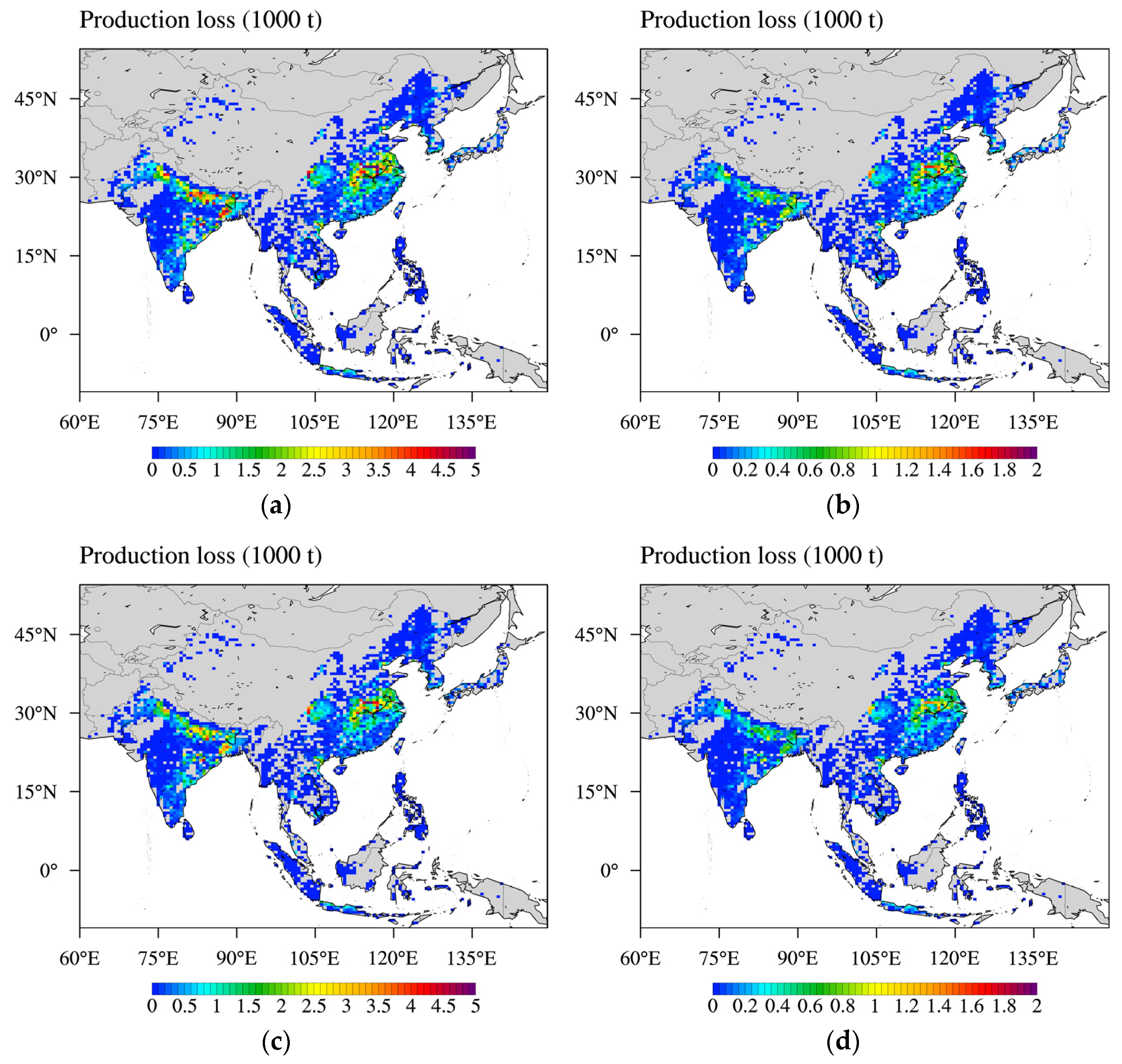
Considering production, the largest RPL area was the India-Gangetic Plain and the Yangtze River basin, which were slightly south of the larger RYL area owing to the overall higher production in the south (Figure 5). The largest aggregated RPL for BASE simulation was observed in China (22,202 Kt on AOT40; 7047 Kt on M7), followed by India (17,322 Kt on AOT40; 3861 Kt on M7), Bangladesh (1183 Kt on AOT40; 491 Kt on M7), Vietnam (1139 Kt on AOT40; 416 Kt on M7), and Pakistan (1117 Kt on AOT40; 325 Kt on M7) (Table 2). The RPL reduction in Asia for CASE 1 compared with BASE simulation was 8956 Kt on AOT40 and 2228 Kt on M7, respectively (Figure 5 and Table 2). This indicates that a 50% reduction in anthropogenic CH4 would reduce losses from the total production in Asia by as much as 1.0% based on AOT40 and 0.3% based on M7.
CH4-induced O3 affects rice yield and production negatively. Therefore, reducing CH4 emissions not only mitigates greenhouse warming but also reduces yield losses due to O3. The highest projected RYL in countries like Bhutan, India, Pakistan, China, and Laos, based on the AOT40 metric, is likely due to anticipated O3 exposure exceeding 40 ppmh during the growth phase. However, it is important to note that the accuracy of this value is uncertain due to the lack of high-resolution O3 studies in Asia for 2010 as a basis for comparison. The study reveals a discrepancy between the RYLs calculated using the AOT40 and M7 metrics. Rice appears to be more O3-resistant according to the M7 metric but sensitive according to the AOT40 metric. This could imply that rice is more vulnerable to short-term, high O3 levels than to prolonged, moderate levels, which is consistent with the findings of Hollaway et al. [55]. Ground level O3 is harmful to rice, and reduced CH4 concentrations increase rice yields.
3.5. Uncertainty from Impacts of Methane Emissions
O3 is generated using the interaction of sunlight with emissions of NOx, CO, NMVOC, and CH4. Furthermore, a certain percentage of tropospheric O3 is transported from the stratosphere. However, there is approximately a 50% uncertainty in the change in O3 owing to CH4 over 40 years calculated using multiple models that allow for the estimation of interactions with NOx and NMVOC degradation chemistry and the resulting radical levels [56]. Notably, 55% of the increase in the O3 budget since the pre-industrial era is ascribed to NOx, with 25% linked to CH4 and 19% to CO and NMVOC [57]. Therefore, CH4 decomposition chemistry and the resulting O3 formation are elucidated using laboratory, field, and modeling knowledge. Though model studies indicate contributions from CH4 to O3 trends, determining whether model performance limits the ability to predict O3 trends is difficult [58,59]. Therefore, the extent to which O3 trends can be attributed to surface CH4 concentration and estimations of the effect of CH4-induced O3 on crop damage are uncertain. The findings of this study provide valuable insights for policymakers, aiding the formulation and implementation of emission control measures targeting O3 precursors to enhance the resilience of future crop yields. While external factors like weather and soil conditions directly impact rice growth, there is a noticeable research gap concerning the synergistic effects of CH4 and O3 levels with meteorological factors, including climate change, on local-scale agricultural production. Therefore, aspects such as long-term surface and troposphere O3 and CH4 observations and model development, including parameterization and process improvement, should be studied further.
4. Conclusions
In this study, the GEOS-Chem model was applied to study rice impacts from CH4-induced O3, as well as the effect of reducing anthropogenic CH4 emissions on rice yield and production across Asia. The average O3-induced RYL for rice in Asia was 9.5% on AOT40 and 2.9% on M7. The O3-induced damage to rice based on AOT40 and M7 were approximately 45,121 Kt and 12,986 Kt, respectively, on a production basis in Asia. Regionally, the Hindustan Plains to the Deccan Plateau and the Yellow River Basin exhibited relatively high RYLs. The Hindustan Plains and Yangtze River basin exhibited a relatively high RPL. Moreover, simulation analysis shows that reducing anthropogenic CH4 emissions mitigates O3 damage to rice production. In Asia, the reduced rice production losses with a 50% reduction in anthropogenic CH4 emission were 8956 Kt for AOT40 and 2228 Kt for M7. Moreover, CH4 control in the BTH in the North China Plain would reduce the effect of O3 pollution on rice yields in high-latitude zones and emphasize the importance of reducing CH4 emissions. The study findings are expected to contribute to the identification of a more effective and environmentally friendly strategy for improving rice production against the backdrop of CH4-induced O3. In addition, this study highlights the pressing necessity for policy initiatives to reduce anthropogenic CH4 emissions, particularly within sectors such as agriculture, fossil fuel production, and waste management. Implementing such measures can effectively mitigate the adverse effects of climate change and substantially curtail crop yield losses, thereby ensuring food security in major rice-producing nations across Asia.
Future research should concentrate on refining O3 response models pertaining to CH4 emissions and improving the accuracy of yield loss predictions. The development of exposure-response relationships with reduced uncertainty will prove pivotal in quantifying the benefits associated with CH4 emission reductions on rice yields and production.
Supplementary Materials
The following supporting information can be downloaded at: https://www.mdpi.com/article/10.3390/atmos14101558/s1, Figure S1: Relative error between observed and simulated surface O3 concentrations for 2010 at (a) January, (b) February, (c) March, (d) April, (e) May, (f) June, (g) July, (h) August, (i) September, (j) October, (k) November, and (l) December. Figure S2: Surface CH4 mixing ratio for 2010 at (a) January, (b) February, (c) March, (d) April, (e) May, (f) June, (g) July, (h) August, (i) September, (j) October, (k) November, and (l) December. Figure S3: Surface O3 mixing ratio for 2010 at (a) January, (b) February, (c) March, (d) April, (e) May, (f) June, (g) July, (h) August, (i) September, (j) October, (k) November, and (l) December. Figure S4: Surface OH mixing ratio for 2010 in (a) January, (b) February, (c) March, (d) April, (e) May, (f) June, (g) July, (h) August, (i) September, (j) October, (k) November, and (l) December. Figure S5: Distribution of surface (a) AOT40 and (b) M7 values for rice production areas for 2010 for CASE 1.
Funding
This research was funded by JST PRESTO, grant number JPMJPR16O3, and JSPS KA-KENHI, grant numbers 16KK0169 and 19K15944.
Institutional Review Board Statement
Not applicable.
Informed Consent Statement
Not applicable.
Data Availability Statement
Data can be made available upon request.
Conflicts of Interest
The author declares no conflict of interest.
References
- Abbas, A.; Waseem, M.; Ahmad, R.; Khan, K.A.; Zhao, C.; Zhu, J. Sensitivity analysis of greenhouse gas emissions at farm level: Case study of grain and cash crops. Environ. Sci. Pollut. Res. 2022, 29, 82559–82573. [Google Scholar] [CrossRef] [PubMed]
- Elahi, E.; Khalid, Z.; Tauni, M.Z.; Zhang, H.; Lirong, X. Extreme weather events risk to crop-production and the adaptation of innovative management strategies to mitigate the risk: A retrospective survey of rural Punjab, Pakistan. Technovation 2022, 117, 102255. [Google Scholar] [CrossRef]
- Lelieveld, J.; Klingmüller, K.; Pozzer, A.; Burnett, R.T.; Haines, A.; Ramanathan, V. Effects of fossil fuel and total anthropogenic emission removal on public health and climate. Proc. Natl. Acad. Sci. USA 2019, 116, 7192–7197. [Google Scholar] [CrossRef] [PubMed]
- Global Monitoring Laboratory. Trends in Atmospheric Methane. 2022. Available online: https://gml.noaa.gov/ccgg/trends_CH4/ (accessed on 25 June 2022).
- Climate and Clean Air Coalition (CCAC); United Nations Environment Programme (UNEP). Global Methane Assessment. 2021. Available online: https://www.ccacoalition.org/en/resources/global-methane-assessment-full-report (accessed on 12 May 2022).
- Jackson, R.B.; Saunois, M.; Bousquet, P.; Canadell, J.G.; Poulter, B.; Stavert, A.R.; Bergamaschi, P.; Niwa, Y.; Segers, A.; Tsuruta, A. Increasing anthropogenic methane emissions arise equally from agricultural and fossil fuel sources. Environ. Res. Lett. 2020, 15, 071002. [Google Scholar] [CrossRef]
- Höglund-Isaksson, L.; Gómez-Sanabria, A.; Klimont, Z.; Rafaj, P.; Schöpp, W. Technical potentials and costs for reducing global anthropogenic methane emissions in the 2050 timeframe –results from the GAINS model. Environ. Res. Commun. 2020, 2, 025004. [Google Scholar] [CrossRef]
- Van Dingenen, R.; Crippa, M.; Janssens-Maenhout, G.; Guizzardi, D.; Dentener, F. Global Trends of Methane Emissions and Their Impacts on Ozone Concentrations; Publications Office of the European Union: Luxembourg, 2018; ISBN 978-92-79-96550-0. [Google Scholar]
- Liu, X.; Desai, A.R. Significant reductions in crop yields from air pollution and heat stress in the United States. Earth’s Future 2021, 9, e2021EF002000. [Google Scholar] [CrossRef]
- Avnery, S.; Mauzerall, D.L.; Liu, J.; Horowitz, L.W. Global crop yield reductions due to surface ozone exposure: 1. Year 2000 crop production losses and economic damage. Atmos. Environ. 2011, 45, 2284–2296. [Google Scholar] [CrossRef]
- Shindell, D.T.; Fuglestvedt, J.S.; Collins, W.J. The social cost of methane: Theory and applications. Faraday Discuss. 2017, 200, 429–451. [Google Scholar] [CrossRef]
- Mills, G.; Sharps, K.; Simpson, D.; Pleijel, H.; Frei, M.; Burkey, K.; Emberson, L.; Uddling, J.; Broberg, M.; Feng, Z.; et al. Closing the global ozone yield gap: Quantification and cobenefits for multistress tolerance. Glob. Change Biol. 2018, 24, 4869–4893. [Google Scholar] [CrossRef]
- United Nations Environment Programme; Climate and Clean Air Coalition. Global Methane Assessment: Benefits and Costs of Mitigating Methane Emissions; United Nations Environment Programme: Nairobi, Kenya, 2021; ISBN 978-92-807-3854-4. [Google Scholar]
- Bey, I.; Jacob, D.J.; Yantosca, R.M.; Logan, J.A.; Field, B.D.; Fiore, A.M.; Li, Q.; Liu, H.Y.; Mickley, L.J.; Schultz, M.G. Global modeling of tropospheric chemistry with assimilated meteorology: Model description and evaluation. J. Geophys. Res. 2001, 106, 23073–23095. [Google Scholar] [CrossRef]
- World Meteorological Organization (WMO). WMO Greenhouse Gas Bulletin—The State of Greenhouse Gases in the Atmosphere Based on Global Observations through 2010; WMO: Geneva, Switzerland, 2011. [Google Scholar]
- Fiore, A.M.; Jacob, D.J.; Field, B.D. Linking ozone pollution and climate change: The case for controlling methane. Geophys. Res. Lett. 2002, 29, 1919. [Google Scholar] [CrossRef]
- Duncan Fairlie, T.; Jacob, D.J.; Park, R.J. The impact of transpacific transport of mineral dust in the United States. Atmos. Environ. 2007, 41, 1251–1266. [Google Scholar] [CrossRef]
- Jaeglé, L.; Quinn, P.K.; Bates, T.S.; Alexander, B.; Lin, J.-T. Global distribution of sea salt aerosols: New constraints from in situ and remote sensing observations. Atmos. Chem. Phys. 2011, 11, 3137–3157. [Google Scholar] [CrossRef]
- Hudman, R.C.; Moore, N.E.; Mebust, A.K.; Martin, R.V.; Russell, A.R.; Valin, L.C.; Cohen, R.C. Steps towards a mechanistic model of global soil nitric oxide emissions: Implementation and space based-constraints. Atmos. Chem. Phys. 2012, 12, 7779–7795. [Google Scholar] [CrossRef]
- Murray, L.T.; Jacob, D.J.; Logan, J.A.; Hudman, R.C.; Koshak, W.J. Optimized regional and interannual variability of lightning in a global chemical transport model constrained by LIS/OTD satellite data. J. Geophys. Res. 2012, 117, D20307. [Google Scholar] [CrossRef]
- van der Werf, G.R.; Randerson, J.T.; Giglio, L.; van Leeuwen, T.T.; Chen, Y.; Rogers, B.M.; Mu, M.; van Marle, M.J.E.; Morton, D.C.; Collatz, G.J.; et al. Global fire emissions estimates during 1997–2016. Earth Syst. Sci. Data 2017, 9, 697–720. [Google Scholar] [CrossRef]
- Guenther, A.B.; Jiang, X.; Heald, C.L.; Sakulyanontvittaya, T.; Duhl, T.; Emmons, L.K.; Wang, X. The Model of Emissions of Gases and Aerosols from Nature version 2.1 (MEGAN2.1): An extended and updated framework for modeling biogenic emissions. Geosci. Model Dev. 2012, 5, 1471–1492. [Google Scholar] [CrossRef]
- Prather, M.; Ehhalt, D.; Dentener, F.; Derwent, R.; Dlugokencky, E.; Holland, E.; Isaksen, I.; Katima, J.; Kirchhoff, V.; Matson, P.; et al. Atmospheric chemistry and greenhouse gases. In Climate Change 2001; Houghton, J.T., Ed.; Cambridge University Press: Cambridge, UK, 2001; pp. 241–279. [Google Scholar]
- Prather, M.J. Time scales in atmospheric chemistry: Theory, GWPs for CH4 and CO, and runaway growth. Geophys. Res. Lett. 1996, 23, 2597–2600. [Google Scholar] [CrossRef]
- Rienecker, M.M.; Suarez, M.J.; Gelaro, R.; Todling, R.; Bacmeister, J.; Liu, E.; Bosilovich, M.G.; Schubert, S.D.; Takacs, L.; Kim, G.-K.; et al. MERRA: NASA’s Modern-Era Retrospective Analysis for Research and Applications. J. Clim. 2011, 24, 3624–3648. [Google Scholar] [CrossRef]
- FAO. GAEZ v4 Data Portal. 2021. Available online: https://gaez.fao.org/pages/data-access-download (accessed on 11 March 2022).
- Sacks, W.J.; Deryng, D.; Foley, J.A.; Ramankutty, N. Crop planting dates: An analysis of global patterns. Glob. Ecol. Biogeogr. 2010, 19, 607–620. [Google Scholar] [CrossRef]
- Monitoring Atmospheric Composition & Climate (MACC). Global Reanalysis of Assimilated Gridded O3 Data at the Surface. Copernicus Atmosphere Monitoring Service. Available online: https://atmosphere.copernicus.eu/catalogue#/ (accessed on 18 March 2023).
- Tai, A.P.K.; Martin, M.V.; Heald, C.L. Threat to future global food security from climate change and ozone air pollution. Nat. Clim. Change 2014, 4, 817–821. [Google Scholar] [CrossRef]
- Emberson, L.D.; Büker, P.; Ashmore, M.R.; Mills, G.; Jackson, L.S.; Agrawal, M.; Atikuzzaman, M.D.; Cinderby, S.; Engardt, M.; Jamir, C.; et al. A comparison of North American and Asian exposure–response data for ozone effects on crop yields. Atmos. Environ. 2009, 43, 1945–1953. [Google Scholar] [CrossRef]
- Tatsumi, K. Rice yield reductions due to ozone exposure and the roles of VOCs and NOx in ozone production in Japan. J. Agric. Meteorol. 2022, 78, 89–100. [Google Scholar] [CrossRef]
- Wang, X.; Mauzerall, D.L. Characterizing distributions of surface ozone and its impact on grain production in China, Japan and South Korea: 1990 and 2020. Atmos. Environ. 2004, 38, 4383–4402. [Google Scholar] [CrossRef]
- Van Dingenen, R.; Dentener, F.J.; Raes, F.; Krol, M.C.; Emberson, L.; Cofala, J. The global impact of ozone on agricultural crop yields under current and future air quality legislation. Atmos. Environ. 2009, 43, 604–618. [Google Scholar] [CrossRef]
- Schiferl, L.D.; Heald, C.L. Particulate matter air pollution may offset ozone damage to global crop production. Atmos. Chem. Phys. 2018, 18, 5953–5966. [Google Scholar] [CrossRef]
- Li, J.; Nagashima, T.; Kong, L.; Ge, B.; Yamaji, K.; Fu, J.S.; Wang, X.; Fan, Q.; Itahashi, S.; Lee, H.-J.; et al. Model evaluation and intercomparison of surface-level ozone and relevant species in East Asia in the context of MICS-Asia Phase III—Part 1: Overview. ACP 2019, 19, 12993–13015. [Google Scholar] [CrossRef]
- Yan, J.; Wang, G.; Yang, P.; Li, D.; Bian, J. Influence of NOx, Cl, and Br on the upper core of the ozone valley over the Tibetan Plateau during summer: Simulations with a box model. Sci. Total Environ. 2022, 817, 152776. [Google Scholar] [CrossRef] [PubMed]
- Liu, Y.; Li, W.; Zhou, X.; He, J. Mechanism of formation of the ozone valley over the Tibetan Plateau in summer—Transport and chemical process of ozone. Adv. Atmos. Sci. 2003, 20, 103–109. [Google Scholar] [CrossRef]
- Han, Z.; Sakurai, T.; Ueda, H.; Carmichael, G.R.; Streets, D.; Hayami, H.; Wang, Z.; Holloway, T.; Engardt, M.; Hozumi, Y.; et al. MICS-ASIA II: Model intercomparison and evaluation of ozone and relevant species. Atmos. Environ. 2008, 42, 3491–3509. [Google Scholar] [CrossRef]
- Nussbaumer, C.M.; Crowley, J.N.; Schuladen, J.; Williams, J.; Hafermann, S.; Reiffs, A.; Axinte, R.; Harder, H.; Ernest, C.; Novelli, A.; et al. Measurement report: Photochemical production and loss rates of formaldehyde and ozone across Europe. Atmos. Chem. Phys. 2021, 21, 18413–18432. [Google Scholar] [CrossRef]
- Lin, X.; Zhang, W.; Crippa, M.; Peng, S.; Han, P.; Zeng, N.; Yu, L.; Wang, G. A Comparative Study of Anthropogenic CH4 Emissions over China Based on the Ensembles of Bottom-Up Inventories. Earth Syst. Sci. Data 2021, 13, 1073–1088. [Google Scholar] [CrossRef]
- Liu, N.; Lin, W.; Ma, J.; Xu, W.; Xu, X. Seasonal variation in surface ozone and its regional characteristics at global atmosphere watch stations in China. J. Environ. Sci. 2019, 77, 291–302. [Google Scholar] [CrossRef] [PubMed]
- Li, K.; Jacob, D.J.; Liao, H.; Shen, L.; Zhang, Q.; Bates, K.H. Anthropogenic drivers of 2013–2017 trends in summer surface ozone in China. Proc. Natl. Acad. Sci. USA 2019, 116, 422–427. [Google Scholar] [CrossRef] [PubMed]
- Kunchala, R.K.; Singh, B.B.; Karumuri, R.K.; Attada, R.; Seelanki, V.; Kumar, K.N. Understanding the spatiotemporal variability and trends of surface ozone over India. Environ. Sci. Pollut. Res. 2022, 29, 6219–6236. [Google Scholar] [CrossRef]
- Deb Roy, S.; Beig, G.; Ghude, S.D. Exposure-plant response of ambient ozone over the tropical Indian region. Atmos. Chem. Phys. 2009, 9, 5253–5260. [Google Scholar] [CrossRef]
- Feng, Z.; Kobayashi, K.; Li, P.; Xu, Y.; Tang, H.; Guo, A.; Paoletti, E.; Calatayud, V. Impacts of current ozone pollution on wheat yield in China as estimated with observed ozone, meteorology and day of flowering. Atmos. Environ. 2019, 217, 116945. [Google Scholar] [CrossRef]
- Marco, A.D.; Anav, A.; Sicard, P.; Feng, Z.; Paoletti, E. High spatial resolution ozone risk-assessment for Asian forests. Environ. Res. Lett. 2020, 15, 104095. [Google Scholar] [CrossRef]
- Sharma, A.; Ojha, N.; Pozzer, A.; Beig, G.; Gunthe, S.S. Revisiting the crop yield loss in India attributable to ozone. Atmos. Environ. X 2019, 1, 100008. [Google Scholar] [CrossRef]
- Cao, J.; Wang, X.; Zhao, H.; Ma, M.; Chang, M. Evaluating the effects of ground-level O3 on rice yield and economic losses in Southern China. Environ. Pollut. 2020, 267, 115694. [Google Scholar] [CrossRef]
- Aunan, K.; Berntsen, T.K.; Seip, H.M. Surface ozone in China and its possible impact on agricultural crop yields. AMBIO J. Hum. Environ. 2000, 29, 294–301. [Google Scholar] [CrossRef]
- Sinha, B.; Singh Sangwan, K.; Maurya, Y.; Kumar, V.; Sarkar, C.; Chandra, B.P.; Sinha, V. Assessment of crop yield losses in Punjab and Haryana using 2 years of continuous in situ ozone measurements. Atmos. Chem. Phys. 2015, 15, 9555–9576. [Google Scholar] [CrossRef]
- Danh, N.T.; Huy, L.N.; Oanh, N.T.K. Assessment of rice yield loss due to exposure to ozone pollution in Southern Vietnam. Sci. Total Environ. 2016, 566–567, 1069–1079. [Google Scholar] [CrossRef] [PubMed]
- Lal, S.; Venkataramani, S.; Naja, M.; Kuniyal, J.C.; Mandal, T.K.; Bhuyan, P.K.; Kumari, K.M.; Tripathi, S.N.; Sarkar, U.; Das, T.; et al. Loss of crop yields in India due to surface ozone: An estimation based on a network of observations. Environ. Sci. Pollut. Res. 2017, 24, 20972–20981. [Google Scholar] [CrossRef] [PubMed]
- Lin, Y.; Jiang, F.; Zhao, J.; Zhu, G.; He, X.; Ma, X.; Li, S.; Sabel, C.E.; Wang, H. Impacts of O3 on premature mortality and crop yield loss across China. Atmos. Environ. 2018, 194, 41–47. [Google Scholar] [CrossRef]
- Zhao, H.; Zheng, Y.; Zhang, Y.; Li, T. Evaluating the effects of surface O3 on three main food crops across China during 2015–2018. Environ. Pollut. 2020, 258, 113794. [Google Scholar] [CrossRef]
- Hollaway, M.J.; Arnold, S.R.; Challinor, A.J.; Emberson, L.D. Intercontinental trans-boundary contributions to ozone-induced crop yield losses in the Northern Hemisphere. Biogeosciences 2012, 9, 271–292. [Google Scholar] [CrossRef]
- Wild, O.; Fiore, A.M.; Shindell, D.T.; Doherty, R.M.; Collins, W.J.; Dentener, F.J.; Schultz, M.G.; Gong, S.; MacKenzie, I.A.; Zeng, G.; et al. Modelling future changes in surface ozone: A parameterized approach. Atmos. Chem. Phys. 2012, 12, 2037–2054. [Google Scholar] [CrossRef]
- Wang, Y.; Jacob, D.J. Anthropogenic forcing on tropospheric ozone and OH since preindustrial times. J. Geophys. Res. 1998, 103, 31123–31135. [Google Scholar] [CrossRef]
- Parrish, D.D.; Petropavlovskikh, I.; Oltmans, S.J. Reversal of Long-Term Trend in Baseline Ozone Concentrations at the North American West Coast. Geophys. Res. Lett. 2017, 44, 10675–10681. [Google Scholar] [CrossRef]
- Derwent, R.G.; Manning, A.J.; Simmonds, P.G.; Spain, T.G.; O’Doherty, S. Long-term trends in ozone in baseline and European regionally-polluted air at Mace Head, Ireland over a 30-year period. Atmos. Environ. 2018, 179, 279–287. [Google Scholar] [CrossRef]
Figure 1.
Diagram of the atmospheric chemistry simulation in the GEOS-Chem model.

Figure 2.
Simulated mean surface (a) CH4 and (b) O3 mixing ratio for major rice producer countries for each month in the BASE simulation for 2010.
Figure 2.
Simulated mean surface (a) CH4 and (b) O3 mixing ratio for major rice producer countries for each month in the BASE simulation for 2010.

Figure 3.
Distribution of surface (a) AOT40 and (b) M7 values for rice production areas for 2010 under BASE simulations.
Figure 3.
Distribution of surface (a) AOT40 and (b) M7 values for rice production areas for 2010 under BASE simulations.
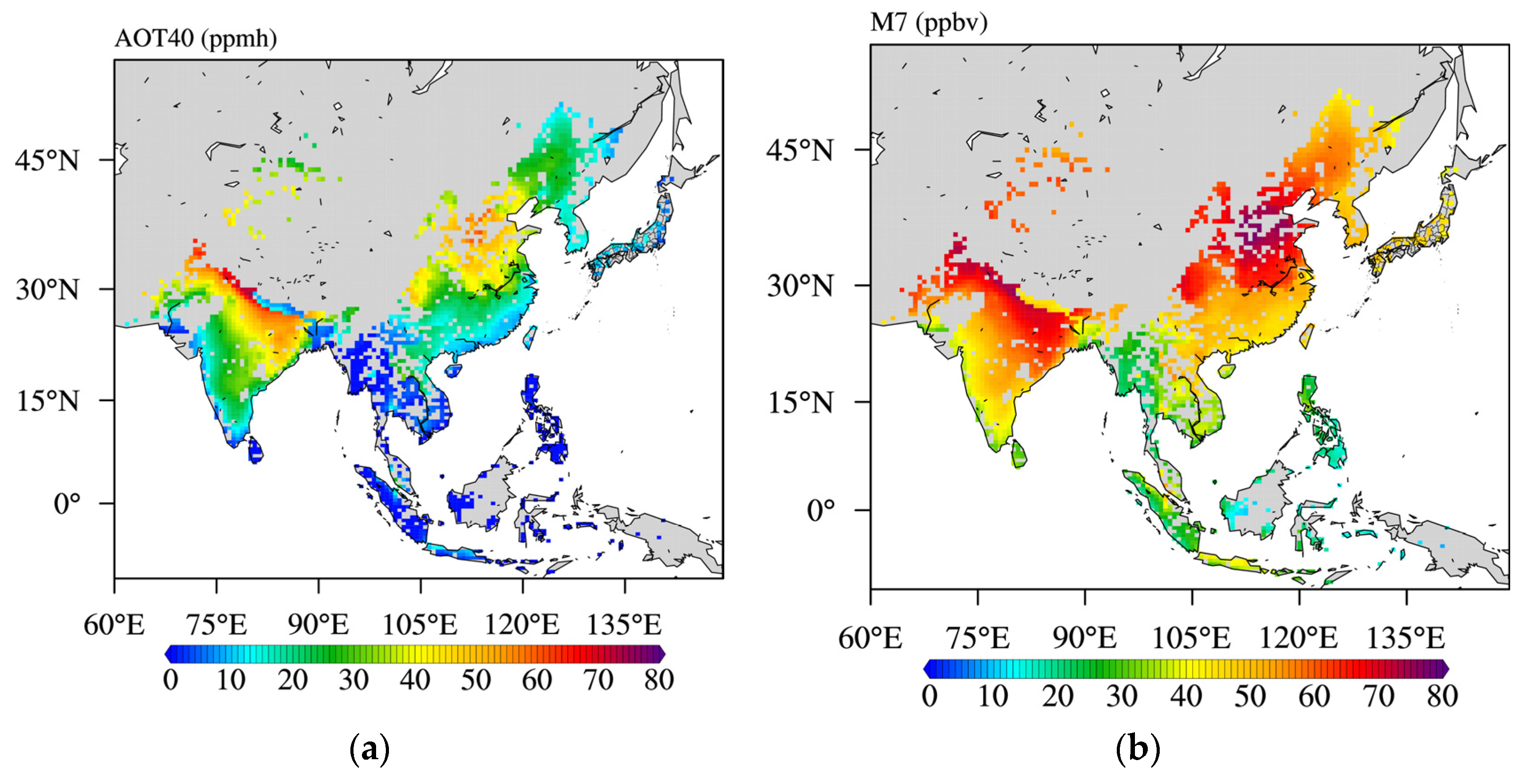
Figure 4.
Relative yield loss (RYL) according to the AOT40 (left) and M7 (right) metrics for 2010. (a,b) BASE, (c,d) CASE1.
Figure 4.
Relative yield loss (RYL) according to the AOT40 (left) and M7 (right) metrics for 2010. (a,b) BASE, (c,d) CASE1.

Figure 5.
Rice production loss (RPL) for 2010 was assessed using the AOT40 (left) and M7 (right) metrics. (a,b) BASE, (c,d) CASE 1.
Figure 5.
Rice production loss (RPL) for 2010 was assessed using the AOT40 (left) and M7 (right) metrics. (a,b) BASE, (c,d) CASE 1.

Table 1.
Simulation cases of methane emissions were used in this study.
| Simulation Name | CH4 Emissions or Mixing Ratio (ppbv) | Reference |
|---|---|---|
| BASE | 1808 | World Meteorological Organization [15] |
| CASE1 | 50% anthropogenic CH4 reduction | Fiore et al. [16] |
Table 2.
Relative yield losses (RYL; %) and rice production losses (RPL; Kt) based on AOT40 (ppmh) and M7 (ppbv) metrics for the year 2010, according to country.
Table 2.
Relative yield losses (RYL; %) and rice production losses (RPL; Kt) based on AOT40 (ppmh) and M7 (ppbv) metrics for the year 2010, according to country.
| Country | BASE | CASE1 | BASE | CASE1 | ||||||||
|---|---|---|---|---|---|---|---|---|---|---|---|---|
| AOT40 | RYL | RPL | AOT40 | RYL | RPL | M7 | RYL | RPL | M7 | RYL | RPL | |
| Japan | 9.1 | 3.8 | 236.1 | 6.8 | 2.8 | 172.8 | 45.5 | 2.0 | 121.5 | 43.2 | 1.6 | 101.2 |
| Republic of Korea | 13.7 | 5.6 | 282.5 | 10.9 | 4.4 | 219.8 | 50.3 | 2.6 | 131.8 | 47.6 | 2.2 | 110.5 |
| North Korea | 15.5 | 6.4 | 136.7 | 12.4 | 5.1 | 108 | 48.2 | 2.3 | 49.1 | 46.0 | 2.0 | 41.8 |
| China | 26.5 | 10.8 | 22,202.0 | 22.3 | 9.1 | 18,296.1 | 55.8 | 3.7 | 7047.2 | 52.9 | 3.2 | 5971.4 |
| Philippines | 0.2 | 0.1 | 8.0 | 0.1 | 0.1 | 5.9 | 21.8 | 0.1 | 7.2 | 20.7 | 0.0 | 4.4 |
| Vietnam | 11.2 | 4.7 | 1138.5 | 9.7 | 4.1 | 949.1 | 41.8 | 1.6 | 416.1 | 39.8 | 1.4 | 348.0 |
| Cambodia | 5.6 | 2.3 | 74.1 | 4.2 | 1.7 | 54 | 34.6 | 0.7 | 23.6 | 32.5 | 0.5 | 16.8 |
| Laos | 19.5 | 8.7 | 94.5 | 17 | 7.5 | 81.9 | 47.1 | 2.4 | 22.9 | 45.1 | 2.1 | 20.0 |
| Thailand | 3.3 | 1.4 | 319.6 | 2.5 | 1.1 | 237.3 | 31.5 | 0.6 | 118.8 | 29.5 | 0.4 | 87.7 |
| Myanmar | 1.0 | 0.4 | 21.9 | 1 | 0.4 | 26.7 | 24.0 | 0.1 | 5.0 | 22.1 | 0.1 | 2.5 |
| Malaysia | 6.3 | 3.3 | 38.8 | 5.4 | 2.8 | 32.4 | 32.4 | 0.9 | 12.0 | 31.0 | 0.8 | 10.3 |
| Indonesia | 1.6 | 0.7 | 541.5 | 1.3 | 0.6 | 428.8 | 25.6 | 0.3 | 215.4 | 24.5 | 0.3 | 177.9 |
| Bangladesh | 8.0 | 3.3 | 1183.3 | 5.9 | 2.4 | 804.5 | 38.2 | 1.2 | 490.6 | 34.9 | 0.8 | 338.8 |
| Nepal | 14.9 | 6.3 | 363.6 | 10.6 | 4.4 | 256.2 | 47.7 | 2.4 | 115.5 | 44.0 | 1.9 | 90.9 |
| Bhutan | 41.5 | 18.6 | 10.3 | 35.1 | 15.8 | 8.4 | 61.4 | 4.8 | 2.2 | 58.1 | 4.1 | 1.9 |
| India | 32.8 | 13.8 | 17,322.4 | 26.8 | 11.2 | 13,645.8 | 53.9 | 3.5 | 3861.4 | 50.5 | 2.9 | 3161.7 |
| Pakistan | 32.3 | 13.6 | 1116.8 | 25.2 | 10.6 | 815.3 | 58.0 | 4.3 | 324.9 | 53.9 | 3.5 | 256.5 |
| Brunei | 0.1 | 0.0 | 0.0 | 0.1 | 0.0 | 0.0 | 25.3 | 0.0 | 0.0 | 24.5 | 0.0 | 0.0 |
| Taiwan | 10.6 | 4.7 | 26.8 | 7.9 | 3.5 | 20.2 | 46.9 | 2.3 | 12.8 | 43.8 | 1.8 | 10.3 |
| Sri Lanka | 0.6 | 0.3 | 2.9 | 0.3 | 0.2 | 1.4 | 31.4 | 0.4 | 8.0 | 29.7 | 0.3 | 5.4 |
| Asia | 22.3 | 9.5 | 45,120.5 | 18.4 | 7.8 | 36,164.6 | 48.5 | 2.9 | 12,985.9 | 45.8 | 2.4 | 10,757.9 |
Disclaimer/Publisher’s Note: The statements, opinions and data contained in all publications are solely those of the individual author(s) and contributor(s) and not of MDPI and/or the editor(s). MDPI and/or the editor(s) disclaim responsibility for any injury to people or property resulting from any ideas, methods, instructions or products referred to in the content. |
© 2023 by the author. Licensee MDPI, Basel, Switzerland. This article is an open access article distributed under the terms and conditions of the Creative Commons Attribution (CC BY) license (https://creativecommons.org/licenses/by/4.0/).
Share and Cite
MDPI and ACS Style
Tatsumi, K. Effect of Surface Methane Controls on Ozone Concentration and Rice Yield in Asia. Atmosphere 2023, 14, 1558. https://doi.org/10.3390/atmos14101558
AMA Style
Tatsumi K. Effect of Surface Methane Controls on Ozone Concentration and Rice Yield in Asia. Atmosphere. 2023; 14(10):1558. https://doi.org/10.3390/atmos14101558
Chicago/Turabian StyleTatsumi, Kenichi. 2023. "Effect of Surface Methane Controls on Ozone Concentration and Rice Yield in Asia" Atmosphere 14, no. 10: 1558. https://doi.org/10.3390/atmos14101558
Note that from the first issue of 2016, this journal uses article numbers instead of page numbers. See further details here.