Article

Determination of Dose–Response Relationship to Derive Odor Impact Criteria for a Wastewater Treatment Plant

1
Tianjin Sinodour Environmental Technology Co., Ltd., Tianjin 300191, China
2
State Environmental Protection Key Laboratory of Odor Pollution Control, Tianjin Academy of Eco-Environmental Sciences, Tianjin 300191, China
3
WG Environmental Health, Unit for Physiology and Biophysics, University of Veterinary Medicine, A-1210 Vienna, Austria
*
Author to whom correspondence should be addressed.
Atmosphere 2021, 12(3), 371; https://doi.org/10.3390/atmos12030371
Submission received: 13 January 2021 / Revised: 2 March 2021 / Accepted: 4 March 2021 / Published: 12 March 2021
(This article belongs to the Special Issue Environmental Odour)

Abstract

:
Municipal wastewater treatment plants (WWTPs) inside cities have been the major complained sources of odor pollution in China, whereas there is little knowledge about the dose–response relationship to describe the resident complaints caused by odor exposure. This study explored a dose–response relationship between the modelled exposure and the annoyance surveyed by questionnaires. Firstly, the time series of odor concentrations were preliminarily simulated by a dispersion model. Secondly, the perception-related odor exposures were further calculated by combining with the peak to mean factors (constant value 4 (Germany) and 2.3 (Italy)), different time periods of “a whole year”, “summer”, and “nighttime of summer”, and two approaches of odor impact criterion (OIC) (“odor-hour” and “odor concentration”). Thirdly, binomial logistic regression models were used to compare kinds of perception-related odor exposures and odor annoyance by odds ratio, goodness of fit and predictive ability. All perception-related odor exposures were positively associated with odor annoyance. The best goodness of fit was found when using “nighttime of summer” in predicting odor-annoyance responses, which highlights the importance of the time of the day and the time of the year weighting. The best predictive performance for odor perception was determined when the OIC was 4 ou/m3 at the 99th percentile for the odor exposure over time periods of nighttime of summer. The study of dose–response relationship could be useful for the odor management and control of WWTP to maximize the satisfaction of air quality for the residents inside city.

1. Introduction

Municipal wastewater treatment plants (WWTPs) as important facilities for urban management have been constructed fast in recent years in China [1]. Unpleasant smells emitted from WWTP may cause both ecological and social problems. Odors are released from pretreatment operations, such as screen and sand filter, primary settler, aeration facility, and sludge de-watering unit in the WWTP. Odor complaints for WWTPs continue to increase by surrounding residents in cities [2]. Although odors are commonly treated as a kind of nuisance, rather than being considered a direct risk for human health, they affect the quality of life and can even cause physical effects on human health [3].
There are many tools to assess odor pollution, some of which include observing the current odor impacts or effects by measurement and monitoring, such as sensorial, analytical, and combined-sensorial technique [4,5] or underlying empirical long-term experiences by community assessment techniques [6,7]. In contrast, other tools make use of a “model” to predict what the impact might be [8,9,10]. Nowadays, most odor assessment regulations all over the world were determined based on the application of dispersion model [11]. In general, different types of models can be used to simulate the dispersion of odorants into the atmosphere, such as empirical model, Gaussian model, Lagrangian particle model and so on. One of the main advantages of Lagrangian particle model is the ability to treat wind calms, it simulates the dispersion of the emitted odorants with computational particles moving in the wind field and three-dimensional turbulence field. [12,13].
Meanwhile, odor impact criterion (OIC) is a jurisdictional standard according to the desired protection level of general population, which aims to compare with simulation exposure in ambient air by air dispersion model [11]. Whereas the limit values of OIC are highly variable in different countries, which related to the national habits, such as 0.25 ou/m3 at the 90th percentile for residential and mixed areas in Germany and 2 ou/m3 for residential areas in Manitoba Canada. This means that the transfer of OIC from other jurisdictions is meaningfulness.
The definition of the OIC depends on several factors, collectively known as the FIDOL factors (frequency, intensity, duration, offensiveness, and location) [14]. In many countries, OICs were defined as the combination of odor concentration threshold (in ou/m3) and exceedance probability (in %), also called percentile [15]. To mimic the odor sensation of the human nose, short-time peak concentrations, which are derived from one hour mean values simulated by dispersion models, can also be included in the criteria [16]. Besides, many factors have been considered to more precisely represent odor annoyance, such as hedonic tones, human psychosocial health, living quality, other environmental stress, age, work, and so on [17]. Furthermore, odor might be perceived more often at specific times, which represent the time of the day and the year can be weighted in odor episodes regarding their annoyance potential [18].
Exposure-annoyance relationship is an important method to study OIC, which has been analysed in industrial sources [19], livestock, agriculture or farming sources [20,21,22,23] and other sources [24,25]. However, there is little knowledge of dose–response relationship describing the resident complaints caused by odor exposure in China. In this work, six odor emitting units of the WWTP were under measurement to identify the time series of odor concentrations for the surrounding residents by an appropriate air dispersion model. Peak to mean factors, temperature and daytime weightings were primarily taken as confounders for coupling with odor concentrations, then two approaches (“odor-hour” and “odor concentration”) of OIC were calculated to transform the time series of odor concentration to the perception-related odor exposures. Meanwhile, community questionnaires were investigated from twelve urban regions surrounding the WWTP to obtain odor annoyance. Dose–response relationship between the perception-related odor exposure and the investigated annoyance was studied by binomial univariate logistic models. It is noticed that the study of dose–response relationship should be useful to determine the OIC for WWTP and other industries in the future.

2. Materials and Methods

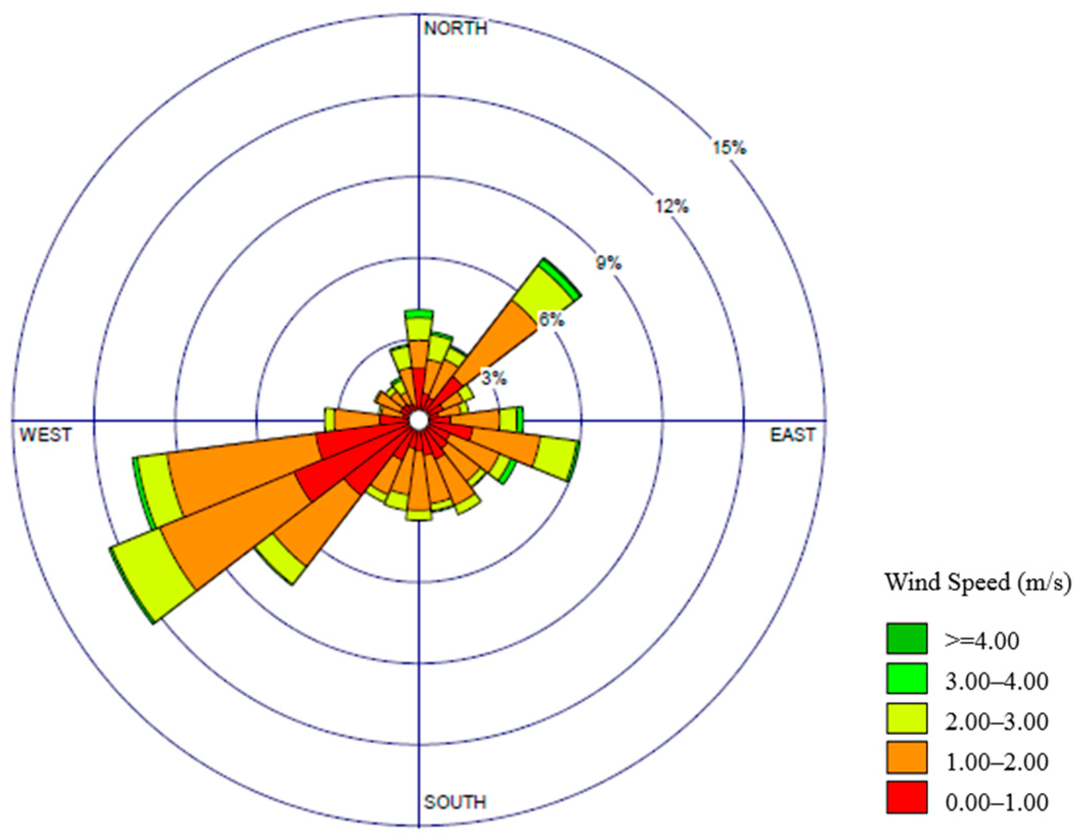
2.1. Site Description and Its Surroundings

The study was conducted at a WWTP located in Northern China, and more precisely in the region of Tianjin. The WWTP was identified as a possible source of nuisance odors, influencing normal life of people living in this area. The distribution of odor complaint incidents during 2017 was shown in Figure 1, derived from environmental protection hotline “12369” of Tianjin, China. On this background, we decided to carry out a specific study by determining a dose–response relationship to derive odor impact criteria of the WWTP.
The WWTP covered about 295,000 m2 and the designed treatment capacity was 400,000 m3/d. It collected wastewater from four administrative regions of Tianjin, served a population of about 1.11 million and 730 enterprises. Six odor emitted units inside this WWTP were selected for analysis. Twelve off-site locations of surrounding residential areas were selected to evaluate odor impact.

2.2. Questionnaire Data Collection

Cross-sectional questionnaire data were obtained from twelve urban regions (Figure 1). A total number of 126 persons were randomly selected and contacted by face-to-face in June 2018. Adult residents (>18 years old) living more than 1 year as being representatives were requested to anonymously participate in the study.
The questionnaire was developed based upon a number of prior investigations [26,27,28] and consisted of two main sections. The first part included general socio-demographic data (i.e., age, gender, address, and years living in the region), while the second part referred to environmental stressors, including satisfaction of living environment and origin of pollution (i.e., noise, traffic, catering, waste, sewage, or others). Regarding the unpleasant smells of sewage, the questions included: degree of perceived odor intensity (estimated using the 6-point scale, i.e., “0 = no odor”,”1 = very faint strength” ”2 = faint strength”, “3 = moderate strength”, “4 = strong strength”, and “5 = very strong strength”), degree of perceived odor annoyance (estimated using the 5-point scale, i.e., “0 = not annoyed”, “1 = slightly annoyed”, “2 = moderately annoyed”, “3 = very annoyed”, and “4 = extremely annoyed”), occurrence time (separated the time of the day into 5 periods, a multiple choice question, i.e., in the morning, at noon, in the afternoon, in the evening, and in the middle of the night), and occurrence season (a multiple choice question, i.e., spring, summer, autumn, and winter).

2.3. Odor Expoure

2.3.1. Sampling Campaign

The air samples were collected according to all odor emitting units of this WWTP, including six treatment processes of screen, sand filter, primary settler, aeration tank, secondary sedimentation, and sludge dewatering unit. Screen and sludge dewatering unit are regarded as point sources, due to these two workshops are completely closed with sealing measures, and the exhaust gas is discharged by chimneys. Sand filter, primary settler, aeration tank, and secondary sedimentation units are regarded as area sources due to the unsealed surfaces (Figure 1). The sampling campaigns were conducted for two days of May and June respectively in 2018, during 8:00 to 18:00, and the total numbers of samples were 24 during the investigation.
The odor samples from point sources were collected by the SOC-01 sampler with “lung” principle (Tianjin Sinodour Environmental Technology Co., Ltd., China) and deposited to a 10 L bio-oriented polyester sample bag equipped with a Teflon TM inlet tube [29]. The odor samplings on area sources were carried out by a wind tunnel system, which consists of a PET hood positioned over the emitting surface. The wind tunnel has a rectangular section inlet and outlet duct (0.042 m × 0.024 m). The central body of the wind tunnel is a 0.5 m wide, 1.0 m long, and 0.13m high rectangular section chamber. The sample stream was filtered through activated carbon at a specific sweep air velocity by a fan, and air sample was collected at the outlet duct with a vacuum pump in 10 L sampling bag [30]. The sweep air velocity inside the wind tunnel remained fixed at 0.064 m s−1.
The gas temperature and exit velocity were measured by thermal anemometer with flow probe (Testo, Germany). The bags were cleaned twice using sample gas before sampling for avoiding the interference of background odor concentration. All samples were sent to the laboratory to analysis within 24 h. Temperature (26–36 °C), humidity (60–90%), and pressure (990–1000 hPa) were measured during the sampling periods by hand-held wind speed and direction indicator (Kestrel, Palo Alto, CA, USA).

2.3.2. Determination of Odor Concentration and Odor Emission Rate

Odor emission rate (OER) is the essential input data for air dispersion modeling and its value directly determines the impact degree on the environmental odor [31]. To evaluate OER, first the calculation of the odor concentration is required.
Odor concentration was measured by the triangle odor bag method in accord with Chinese regulation: Air quality—Determination of odor -Triangle Odor Bag Method [32]. A sniff team of six trained panelists, distinguished the odor from three bags with one odor sample and two odor free air samples. When a given panel member provided an incorrect answer and a correct answer in adjacent dilution ratio, the test for this panel was considered finished, then the personal olfactory threshold was calculated. Finally, the odor concentration was calculated according to the personal olfactory threshold of the six sniff members.
The calculation methods of OER for point source and area source were shown in Equations (1) and (2).
OER1 = C∙V
OER2 = (C∙L/S1)∙S
where OER1, OER2 is the odor emission rate for point source and area source respectively, OU/s; C is the odor concentration, ou/m3; V is the flow rate measured by the gas flow meter, m3/s; L is the flow rate in the outlet duct of wind tunnel system, m3/s; S1 is the base area of wind tunnel, m2; S is the total area of emitting surface, m2.

2.3.3. Odor Dispersion Model

The odor release was calculated by a Lagrange puff model, the CALPUFF model. There were several scientific studies proved the possibility of applying CALPUFF for modelling the dispersion of odorants [33,34]. Puff models represent a continuous plume as a number of discrete packets of pollutant and evaluate the contribution of a puff to the concentration at a receptor by a “snapshot” approach. The basic equation for the contribution of a puff to the concentration at a receptor is expressed in Equations (3) and (4):
C = Q 2 π σ y σ z g   e x p ( d a 2 2 σ x 2 ) e x p ( d c 2 2 σ y 2 )
g = 2 ( 2 π ) 1 / 2 σ z n = e x p [ ( H c + 2 n h ) 2 / ( 2 σ z 2 ) ]
where C is the ground-level odor or pollutant concentration, ou/m3 or mg/m3, Q is the odor or pollutant mass in the puff, OU or mg, σx is the standard deviation of the Gaussian distribution in the along-wind direction, m, σy is the standard deviation of the Gaussian distribution in the cross-wind direction, m, σz is the standard deviation of the Gaussian distribution in the vertical direction, m, da is the distance from the puff center to the receptor in the along-wind direction, m, dc is the distance from the puff center to the receptor in the cross-wind direction, m, g is the vertical term of the Gaussian equation, s/m, H is the effective height above the ground of the puff center, m, and h is the mixing height, m.
The meteorological data used for the study area consisted of two parts, surface meteorological data and upper-air meteorological data, both were from 31 December 2016 to 31 December 2017. Surface meteorological data such as wind direction, wind speed, air pressure, temperature, relative humidity, and cloud cover were obtained from the weather station, which was the nearest one from the WWTP. Upper-air meteorological data were generated by WRF (Weather Research and Forecasting) model with 1 km resolution relevant to the studied area. The wind rose diagram at the WWTP was shown in Figure 2.
Geophysical data (flat terrain, urban area) and grids (nested grids, assessment squares defined by 32 × 32 km2 with the smallest 50 m spacing) were taken as input data in the model. 126 sensitive points were set in the model according to urban resident sites investigated by questionnaires. Then a time serious of one hour mean values of the odor concentrations were calculated at each household, where the corresponding questionnaire was available.

2.4. Perception-Related Odor Exposure Analysis

2.4.1. Preliminary Perception-Related Odor Exposure Variables

Preliminary perception-related exposure variables were determined for weighting the odor concentrations by the following confounders:
(1)
Peak-to-mean factor (F): In regard to the duration of one single human breath, the short-term concentration fluctuations were transformed from one hour mean values of the odor concentrations (e.g., constant value 4 (Germany), 2.3 (Italy) or 1 (UK)) [15];
(2)
Temperature and daytime: The annoyed time period of the year and time period of the day were obtained by the community questionnaires to emphasize those hourly values, when residents are more sensitive to odor.
By these confounders, the odor concentrations were transformed to the perception-related odor exposure preliminarily at each site.

2.4.2. Perception-Related Odor Exposures by OICs

In order to determine which OIC shows a better performance, the “odor-hour” metric approach, expressed as the threshold of a certain percentile (like in Ireland [15]) and the “odor concentration “approach, expressed as the threshold of a certain concentration (like in Germany [15]) were used to calculate the further perception-related odor exposures, which are shown as follows.
(1)
The threshold of a certain percentile at a certain site: The odor concentrations at 98, 95, 90, 85, 80, and 70 percentiles were selected, based on the time series of the preliminary perception-related odor concentrations, expressed as C98, C95, C90, C85, C80, and C70, respectively;
(2)
The threshold of a certain concentration at a certain site: The probabilities exceeding odor concentration thresholds of 1, 2, 3, 4, and 5 ou/m3 were selected, based on the time series of the preliminary perception-related odor concentrations, expressed as P1, P2, P3, P4, and P5, respectively.
Then the further perception-related odor exposures by different OICs were calculated at 126 sensitive points (households).

2.5. Dose–Response Relationship Analysis

Binomial logistic regression models basing on log-logit sigmoid equations were used to estimate the association between the perception-related odor exposures (i.e., C98, C95, C90, C85, C80, C70, P1, P2, P3, P4, and P5, respectively) and the odor annoyances which were derived from questionnaires. For binomial models, the outcome variables of odor annoyance degrees were dichotomized into two scores (score = 0, derived from “not annoyed”, “slightly annoyed”; and score = 1, derived from “moderately annoyed”, “very annoyed”, and “extremely annoyed”). As well, the independent variables of perception-related odor exposures were transformed into loge values, which is due to a log fit between odor exposure and odor annoyance previously was found to be closer than a linear fit [21].
In this analysis, the associations for the dose–response relationships were estimated by OR (odds ratio), 95% CI (confidence interval), and P (significance level). The goodness of fit (Akaike information criterion, AIC; McFadden R2; Hosmer-Lemeshow test, HL test) were obtained. The predictive abilities were also investigated by using AUC (area under the ROC (receiver operating characteristic) curve) and accuracy parameter. The statistical analyses were performed in both SPSS and MATLAB software.

3. Results and Discussion

3.1. Socio-Demographic Characteristics of Participants

The long-term experiences of the communities were investigated and a total of 126 valid questionnaires were obtained in the study. The number of questionnaires in each investigated residential area was shown in Table 1. In general, 60 respondents were females and 66 respondents were males; About 64% of respondents were over the age of 45, about 36% of respondents were at the age of ranging 18 to 45; 68 respondents were living in the household lower than 5 years, 34 respondents were living between 5 to 10 years, and 24 respondents were living more than 10 years; Besides sewage smells, 7 respondents were influenced by noise impact and 13 respondents experienced environmental stressor of waste smells.
In the 126 questionnaires, about 40% of the residents were annoyed by sewage odor at their households, which consist of “moderately annoyed”, “very annoyed”, and “extremely annoyed”, and about 23% of the residents were annoyed as “very annoyed” and “extremely annoyed”. Besides, summer was the most serious annoyed season when sewage smell occurred (20%, 50%, 18%, and 12% was the proportion of occurrence time in spring, summer, autumn, and winter month, respectively). Nighttime was the most serious annoyed time in the day when sewage smell occurred (13%, 10%, 21%, 46%, and 10% was the proportion of occurrence time in the morning, noon, afternoon, night, and midnight of the day, respectively). Odor complaints occur predominantly in the afternoon and evening hours of the warm season when residents are outside [18].
Respondents who lived in residential area A annoyed the most by sewage smell, followed by residential areas C, E, F, and G; Averaged odor intensities in residential areas A-G were all higher to 2, indicated that many people in these residential areas can perceive sewage smell; A small number of people may perceive sewage smell in residential areas H, I, K, which were located on the southwest and 650 m~1100 m away from the WWTP boundary (Table 1).

3.2. Odor Exposure and Perception-Related Odor Exposure

The time series of the odor concentrations were calculated over 8760 h. The average odor concentrations of the 8760 h for 126 sensitive points ranged from 0.3 ou/m3 to 4.8 ou/m3. The order of mean odor concentration from highest to lowest was residential area A (3.7), B (3.6), C (2.7), D (1.3), L (1.2), E (1.1), G (0.8), J (0.8), I (0.5), F (0.5), K (0.5), and H (0.4).
The time series of the odor concentrations were firstly multiplied by peak to mean factors 1, 2.3, and 4, respectively, and divided into three time periods of “a whole year”, “summer”, and “nighttime of summer”, respectively, due to the serious annoyed season of the year and time of the day obtained from the community questionnaires. Then the odor exposures were calculated by “odor concentration“ metric approach, expressed as C98, C95, C90, C85, C80, and C70, respectively, and “odor-hour” metric approach, expressed as P1, P2, P3, P4, and P5, respectively. Based on these calculations, the groups of perception-related odor exposures were obtained.

3.3. Dose–Response Relationship by Binomial Univariate Logistic Models

The perception-related odor exposures and investigated odor annoyances were performed to establish dose–response associations by binomial univariate logistic models. Results revealed the associations between odor annoyance and (1) odor concentrations (C98, C95, C90, C85, C80, and C70); (2) odor percentiles (P1, P2, P3, P4, and P5) (Table 2).
The values of OR were invariant for a certain concentration combined with different constant values of peak to mean factor due to the multiple relations. In regard to the results basing on “a whole year” confounder, all odor exposure variables were positively associated with odor annoyance. C98 as exposure assessment variable seemed to be a slightly better association than other odor concentrations (OR = 2.652; 95% CI =1.493–4.712), and P1 combined with F = 4 showed the greatest correlation (OR = 18.103; 95% CI = 4.204–77.954). Furthermore, the associations were substantially larger when using “odor-hour” metric approach than “odor concentration” approach.
Then the analysis was performed basing on “summer” and “nighttime of summer” confounders. All odor exposure variables were also positively associated with odor annoyance. The strongest association was found when using the combination of P1, F =4, and “nighttime of summer” as exposure assessment variable (e.g., OR = 20.836, 95% CI: 5.077–85.516). Besides, the highest association between odor concentration and odor annoyance was found when using the combination of C98 and “nighttime of summer” (OR = 4.085, 95% CI: 2.128–7.843).

3.4. Goodness of Fit and Predictive Ability of Binomial Logistic Models

The goodness of fit obtained from “nighttime of summer” showed to be preferable in the combination of P2 and F = 1 (AIC = 152.9, McFadden R2 = 0.131 and HL test = 0.215 and the combination of P4 and F = 1 (AIC = 153.0, McFadden R2 = 0.131 and HL test = 0.063) (Table 3). The predictive ability of accuracy and AUC of logistic models seemed not accordance with each other (Table 4). The best accuracy was obtained in the combination of C98 and “summer” and the combination of P4, F = 1 and “nighttime of summer” (accuracy = 66.7). However, the best consequence of AUC was obtained in the combination of C95 and “nighttime of summer” (AUC = 0.743). On the whole, goodness of fit (AIC, McFadden R2) and predictive ability (AUC) showed that the values obtained by “summer” and “nighttime of summer” had better predictive performance than “a year”, especially by “nighttime of summer”. The results illuminate that the odor episode should be weighted by the time of the day and the time of the year when studying odor annoyance, OICs, and so on.

3.5. Odor Impact Criteria of the WWTP

The best predictor of odor exposure was selected as the combination of P4, F = 1, and “nighttime of summer”, integrating goodness of fit and predictive ability. The univariate binomial logistic function was shown in Equation (5). Furthermore, in order to visualize the results of the logistic function, the dose–response curve was shown in Figure 3.
p = 1 + exp (−1.595 − 0.880 lnP4)
where p is the probability of odor annoyance, 0–1; P4 is the probability exceeded odor concentration thresholds of 4 ou/m3, calculated by air dispersion model over the time period of nighttime of summer, %.
Aiming to limit the percentage of people experiencing some form of odor-induced annoyance to 10% or less [35,36], the target value of OIC was calculated as follows: 4 ou/m3 at the 99th percentile for the odor exposure calculated by air dispersion model over the time period of nighttime of summer.

3.6. Lagrange Dispersion Model and Separation Distances

A generalized non-steady-state air quality modeling system for regulatory use, Sigma Research Corporation developed the CALPUFF dispersion model and programs. The model contains algorithms for near-source effects such as building downwash, transitional plume rise, partial plume penetration, subgrid scale terrain interactions, as well as longer range effects such as pollutant removal (wet scavenging and dry deposition), chemical transformation, vertical wind shear, overwater transport, and coastal interaction effects. Most of the algorithms contain options to treat the physical processes at different levels of detail depending on the model application [37]. CALPUFF model is driven by temporally and spatially varying meteorological data on hourly basis, which can handle continuous puffs of pollutants being emitted from a source into the ambient wind flow.
Capelli et al. [13] discussed the preference of the Lagrangian CALPUFF model, due to the limitations of Gaussian models (inability to handle calm conditions, lack of three-dimensional meteorology, and steady-state assumption). In a calibration study of Rood [38], the CALPUFF model showed the smallest variance, highest correlation, and highest number of predictions within a factor of two compared to the AERMOD model. Even for odorous substances, CALPUFF was compared with other dispersion models with good results [39].
Direction-dependent separation distances are commonly used procedure to avoid odor annoyance between emission sources and residential areas, calculated by air dispersion model [40]. The separation distances were simulated by CALPUFF model, basing on the OIC (4 ou/m3 at the 99th percentile for the odor exposure over the time period of nighttime of summer). As shown in Figure 4, residential areas A, B, C, D, E, G, and J were completely annoyed by sewage odors, which was basically accorded with the results of odor complaints in 2017. Besides, a number of people in residential areas F, H, I, K, and L were annoyed, and the separation distance in west-south direction was about 900 m from the WWTP boundary.

4. Conclusions

In conclusion, this was supposed be the first study aimed at determining a certain OIC using different perception-related odor exposure approaches to study dose–response relationship by binomial logistic regression models. The odor exposures calculated over time period of “nighttime of summer” showed better predictive performance than “a whole year” and “summer” in predicting odor-annoyance responses. OIC was taken as 4 ou/m3 at the 99th percentile for the odor exposure calculated by air dispersion model over the time period of nighttime of summer. Furthermore, the separation distances of the WWTP were calculated by CALPUFF model basing on the OIC, which was about 900 m from the WWTP boundary in the west-south direction.

Author Contributions

Conceptualization, G.S.; methodology, W.Y., G.W. and J.M.; formal analysis, Y.Z., W.Y., J.G. and J.W.; data curation, Y.Z., W.Y. and J.W.; writing—original draft preparation, Y.Z.; writing—review and editing, Y.Z. and G.S.; visualization, Y.Z.; supervision, W.Y.; funding acquisition, W.Y. All authors have read and agreed to the published version of the manuscript.

Funding

This research was funded by Natural Science Foundation of Tianjin City, grant number 18JCQNJC08800.

Informed Consent Statement

Informed consent was obtained from all subjects involved in the study.

Conflicts of Interest

The authors declare no conflict of interest.

References

  1. Wang, X.D.; Wang, B.G.; Zhao, D.J.; Liu, S.L. Sources and components of MVOC from a municipal sewage treatment plant in Guangzhou. China Environ. Sci. 2011, 31, 576–583. [Google Scholar]
  2. Stuetz, R.M.; Fenner, R.A.; Engin, G. Assessment of odours from sewage treatment works by an electronic nose, H2S analysis and olfactometry. Water Res. 1999, 33, 453–461. [Google Scholar] [CrossRef]
  3. Han, Z.; Qi, F.; Wang, H.; Li, R.; Sun, D. Odor assessment of NH3 and volatile sulfide compounds in a full-scale municipal sludge aerobic composting plant. Bioresour. Technol. 2019, 282, 447–455. [Google Scholar] [CrossRef] [PubMed]
  4. Barczak, R.J.; Kulig, A. Comparison of different measurement methods of odour and odorants used in the odour impact assessment of wastewater treatment plants in Poland. Water Sci. Technol. 2017, 75, 944–951. [Google Scholar] [CrossRef]
  5. Lim, J.H.; Cha, J.S.; Kong, B.J.; Baek, S.H. Characterization of odorous gases at landfill site and in surrounding areas. J. Environ. Manag. 2018, 206, 291–303. [Google Scholar] [CrossRef]
  6. Mohamed, E.; Shelly, M. Industrial odor source identification based on wind direction and social participation. Int. J. Environ. Res. Public Health 2019, 16, 1242. [Google Scholar]
  7. Hayes, J.E.; Fisher, R.M.; Stevenson, R.J.; Mannebeck, C.; Stuetz, R.M. Unrepresented community odour impact: Improving engagement strategies. Sci. Total Environ. 2017, 609, 1650–1658. [Google Scholar] [CrossRef]
  8. Brancher, M.; Piringer, M.; Franco, D.; Filho, P.B.; Lisboa, H.D.M.; Schauberger, G. Assessing the inter-annual variability of separation distances around odour sources to protect the residents from odour annoyance. J. Environ. Sci. 2019, 79, 11–24. [Google Scholar] [CrossRef]
  9. Douglas, P.; Hayes, E.T.; Williams, W.B.; Tyrrel, S.F.; Kinnersley, R.P.; Walsh, K.; Driscolle, M.O.; Longhurst, P.J.; Pollard, S.J.T.; Drew, G.H. Use of dispersion modelling for environmental impact assessment of biological air pollution from composting: Progress, problems and prospects. Waste Manag. 2017, 70, 22–29. [Google Scholar] [CrossRef] [PubMed]
  10. Pandey, G.; Sharan, M. Performance evaluation of dispersion parameterization schemes in the plume simulation of FFT-07 diffusion experiment. Atmos. Environ. 2018, 172, 32–46. [Google Scholar] [CrossRef]
  11. Piringer, M.; Knauder, W.; Petz, E.; Schauberger, G. A comparison of separation distances against odour annoyance calculated with two models. Atmos. Environ. 2015, 116, 22–35. [Google Scholar] [CrossRef]
  12. Sironi, S.; Capelli, L.; Centola, P.; Rosso, R.D. Odour impact assessment by means of dynamic olfactometry, dispersion modelling and social participation. Atmos. Environ. 2010, 44, 354–360. [Google Scholar] [CrossRef]
  13. Capelli, L.; Sironi, S.; Del Rosso, R.; Guillot, J.M. Measuring odours in the environment vs. dispersion modelling: A review. Atmos. Environ. 2013, 79, 731–743. [Google Scholar] [CrossRef]
  14. Sommer-Quabach, E.; Piringer, M.; Petz, E.; Schauberger, G. Comparability of separation distances between odour sources and residential areas determined by various national odour impact criteria. Atmos. Environ. 2014, 95, 20–28. [Google Scholar] [CrossRef]
  15. Brancher, M.; Griffiths, K.D.; Franco, D.; De Melo Lisboa, H. A review of odour impact criteria in selected countries around the world. Chemosphere 2017, 168, 1531–1570. [Google Scholar] [CrossRef] [PubMed]
  16. Piringer, M.; Schauberger, G.; Mikovits, C.; Zollitsch, W.; Hörtenhuber, S.J.; Baumgartner, J.; Schönhart, M. Climate change impact on the dispersion of airborne emissions and the resulting separation distances to avoid odour annoyance. Atmos. Environ. X 2019, 2, 100021. [Google Scholar] [CrossRef]
  17. Schauberger, G.; Piringer, M.; Schmitzer, R.; Kamp, M.; Sowa, A.; Koch, R.; Eckhof, W.; Grimm, E.; Kypke, J.; Hartung, E. Concept to assess the human perception of odour by estimating short-time peak concentrations from one-hour mean values. Reply to a comment by Janicke et al. Atmos. Environ. 2012, 54, 624–628. [Google Scholar] [CrossRef]
  18. Schauberger, G.; Piringer, M.; Petz, E. Odour episodes in the vicinity of livestock buildings: A qualitative comparison of odour complaint statistics with model calculations. Agric. Ecosyst. Environ. 2006, 114, 185–194. [Google Scholar] [CrossRef]
  19. Li, J.; Zou, K.; Li, W.; Wang, G.; Yang, W. Olfactory Characterization of Typical Odorous Pollutants Part I: Relationship between the Hedonic Tone and Odor Concentration. Atmosphere 2019, 10, 524. [Google Scholar] [CrossRef] [Green Version]
  20. Miedema, H.M.E.; Walpot, J.I.; Vos, H. Exposure-annoyance relationships for odour from industrial sources. Atmos. Environ. 2000, 34, 2927–2936. [Google Scholar] [CrossRef]
  21. Blanes-Vidal, V.; Baelum, J.; Nadimi, E.S.; Løfstrøm, P.; Christensen, L.P. Chronic exposure to odorous chemicals in residential areas and effects on human psychosocial health: Dose–response relationships. Sci. Total Environ. 2014, 490, 545–554. [Google Scholar] [CrossRef]
  22. Cantuaria, M.L.; Lofstrom, P.; Blanes-Vidal, V. Comparative analysis of spatio-temporal exposure assessment methods for estimating odor-related responses in non-urban populations. Sci. Total Environ. 2017, 605–606, 702–712. [Google Scholar] [CrossRef]
  23. Moshammer, H.; Oettl, D.; Mandl, M.; Kropsch, M.; Weitensfelder, L. Comparing annoyance potency assessments for odors from different livestock animals. Atmosphere 2019, 10, 659. [Google Scholar] [CrossRef] [Green Version]
  24. Sucker, K.; Both, R.; Bischoff, M.; Guski, R.; Krämer, U.; Winneke, G. Odor frequency and odor annoyance Part II: Dose–response associations and their modification by hedonic tone. Int. Arch. Occup. Environ. Heath 2008, 81, 683–694. [Google Scholar] [CrossRef] [PubMed]
  25. Weitensfelder, L.; Moshammer, H.; Dietmar, O.; Payer, I. Exposure-complaint relationships of various environmental odor sources in Styria, Austria. Environ. Sci. Pollut. Res. 2019, 26, 9806–9815. [Google Scholar] [CrossRef] [PubMed] [Green Version]
  26. Verein Deutscher Ingenieure. Determination of Annoyance Parameters by Questioning Repeated Brief Questioning of Neighbour Panelists (VDI3883 Part 2); Beuth Verlag GmbH: Berlin, Germany, 1993. [Google Scholar]
  27. Hayes, J.E.; Stevenson, R.J.; Stuetz, R.M. Survey of the effect of odour impact on communities. J. Environ. Manag. 2017, 204, 349–354. [Google Scholar] [CrossRef] [PubMed]
  28. Miedema, H.M.E.; Ham, J.M. Odour annoyance in residential areas. Atmos. Environ. 1988, 22, 2501–2507. [Google Scholar] [CrossRef]
  29. Mustafa, M.F.; Liu, Y.; Duan, Z.; Guo, H.; Xu, S.; Wang, H.; Lu, W. Volatile compounds emission and health risk assessment during composting of organic fraction of municipal solid waste. J. Hazard Mater. 2016, 327, 35–43. [Google Scholar] [CrossRef]
  30. Jiang, K.; Bliss, P.J.; Schulz, T.J. The development of a sampling system for determining odor emission rates from areal surfaces: Part I. aerodynamic performance. J. Air Waste Manag. Assoc. 1995, 45, 917–922. [Google Scholar] [CrossRef]
  31. Lucernoni, F.; Tapparo, F.; Capelli, L.; Sironi, S. Evaluation of an odour emission factor (OEF) to estimate odour emissions from landfill surfaces. Atmos. Environ. 2016, 144, 87–99. [Google Scholar] [CrossRef]
  32. Ministry of Ecology and Environment of China (MEEC). Air Quality-Determination of Odor-Triangle Odor Bag Method (GB 1467593); Ministry of Ecology and Environment of China: Beijing, China, 1993.
  33. Capelli, L.; Selena, S. Combination of field inspection and dispersion modelling to estimate odour emissions from an Italian landfill. Atmos. Environ. 2018, 191, 273–290. [Google Scholar] [CrossRef] [Green Version]
  34. Businia, V.; Capelli, L.; Sironi, S. Comparison of CALPUFF and AERMOD models for odour dispersion simulation. Chem. Eng. Trans. 2012, 30, 205–210. [Google Scholar]
  35. Invernizzi, M.; Brancher, M.; Sironi, S.; Capelli, L.; Piringer, M.; Schauberger, G. Odour impact assessment by considering short-term ambient concentrations: A multi-model and two-site comparison. Environ. Int. 2020, 144, 105990. [Google Scholar] [CrossRef]
  36. Bull, M.; McIntyre, A.; Hall, D. Guidance on the Assessment of Odour for Planning v1.1; IAQM: London, UK, 2018. [Google Scholar]
  37. Scire, J.S.; Strimaitis, D.G.; Yamartino, R.J. A user’s guide for the CALPUFF dispersion model. Earth Tech. Inc. 2000, 521, 1–521. [Google Scholar]
  38. Rood, A. Performance evaluation of AERMOD, CALPUFF, and legacy air dispersion models using the Winter Validation Tracer Study dataset. Atmos. Environ. 2014, 89, 707–720. [Google Scholar] [CrossRef] [Green Version]
  39. Yu, Z.; Guo, H.; Laguë, C. Development of a livestock odor dispersion model: Part II. Evaluation and validation. J. Air Waste Manag. Assoc. 2011, 61, 277–284. [Google Scholar] [CrossRef] [PubMed] [Green Version]
  40. Wu, C.; Brancher, M.; Yang, F.; Liu, J.; Qu, C.; Schauberger, G.; Piringer, M. A comparative analysis of methods for determining odour-related separation distances around a dairy farm in Beijing, China. Atmosphere 2019, 10, 231. [Google Scholar] [CrossRef] [Green Version]
Figure 1. The location of the wastewater treatment plant (WWTP) and twelve surrounding residential areas (AL). The yellow stars which located in seven residential areas (A), (CG), and (J) represent the major off-site locations of odor complaints. The distance between the boundary of plant and the southwest corner of residential area K is about 1.2 km. WWTP: Municipal wastewater treatment plant.
Atmosphere 12 00371 g001
Figure 2. Wind rose diagram in the atmospheric vertical altitude of 10 m at the WWTP during 2017. Legend denotes wind speed categories and their associated colors. WWTP: Municipal wastewater treatment plant.
Atmosphere 12 00371 g002
Figure 3. Exposure–response univariate binomial logistic model between odor exposure and probability of odor annoyance; The odor exposure of P4 is the probability exceeded odor concentration thresholds of 4 ou/m3, calculated by air dispersion model over the time period of nighttime of summer, %; F: Peak-to-mean factor.
Atmosphere 12 00371 g003
Figure 4. Direction-dependent separation distances based on the odor impact criterion (OIC) by air dispersion model. OIC: 4 ou/m3 at the 99th percentile for the odor exposure calculated over the time period of nighttime of summer.
Atmosphere 12 00371 g004
Table 1. The questionnaire number, averaged odor intensity and odor annoyance by respondents in investigated residential areas A–L.
Title Questionnaire ResultInvestigated Residential Area
ABCDEFGHIGKL
Questionnaire number101012131111121011121015
Averaged odor intensity2.82.52.83.03.02.42.10.80.82.50.71.4
Odor annoyance (%)75336445635544111050029
Table 2. OR values for odor annoyance by binomial logistic regression models a,b.
Odor ConcentrationPeak to Mean FactorVariable of Odor Exposure: The Threshold of Concentration
Modeled by a YearModeled by SummerModeled by Nighttime of Summer
C704/2.3/12.0631.433–2.9711.9671.440–2.6881.7571.347–2.293
C804/2.3/12.4381.577–3.7702.4811.630–3.7142.2541.553–3.273
C854/2.3/12.2791.499–3.4662.3081.557–3.4162.4021.589–3.633
C904/2.3/12.1931.398–3.4392.3651.534–3.6472.4751.597–3.835
C954/2.3/12.2781.408–3.6872.4731.543–3.9643.1531.870–5.316
C984/2.3/12.6521.493–4.7123.4481.855–6.4094.0852.128–7.843
Odor PercentilePeak to Mean FactorVariable of Odor Exposure: The Threshold of Percentile
Modeled by a YearModeled by SummerModeled by Nighttime of Summer
P117.4032.674–20.4996.2872.659–14.8678.3623.135–22.307
2.311.7913.363–41.3438.2773.065–22.35613.8213.987–47.902
418.1034.204–77.95410.9423.591–33.33820.8365.077–85.516
P213.8141.842–7.8934.2572.119–8.5513.8402.021–7.295
2.37.8742.767–22.4126.3712.677–15.1628.7193.163–24.036
410.3453.134–34.1487.6272.936–19.81212.6773.833–41.931
P312.5941.515–4.4403.0661.769–5.3132.8241.743–4.576
2.36.9022.585–18.4286.0142.604–13.8927.1102.876–17.575
48.5362.882–25.2836.6812.759–16.1779.7353.366–28.156
P412.1771.383–3.4282.5551.601–4.0772.4111.606–3.619
2.34.8512.118–11.1074.9862.351–10.5744.7592.287–9.901
47.4032.674–20.4996.0322.603–13.9818.3623.135–22.307
P511.9501.309–2.9062.2311.486–3.3492.1431.496–3.070
2.33.4481.747–6.8063.7761.975–7.2203.5271.934–6.430
46.9342.589–18.5755.8342.557–13.3077.2982.916–18.262
a Odor exposures were loge transformed; b p Values were all lower than 0.001.
Table 3. Goodness of fit (AIC, McFadden R2, HL test) for odor annoyance by binomial logistic regression models a.
Odor ConcentrationPeak to Mean FactorVariable of Odor Exposure: The Threshold of Concentration
Modeled by a YearModeled by SummerModeled by Nighttime of Summer
AICMcFadden R2HL TestAICMcFadden R2HL TestAICMcFadden R2HL Test
C704/2.3/1157.60.1050.335154.30.1240.083154.80.1210.104
C804/2.3/1156.50.1100.045153.10.1300.028153.50.1280.107
C854/2.3/1158.60.0990.098155.10.1190.016155.50.1170.073
C904/2.3/1162.70.0750.102162.70.0750.032156.70.1090.050
C954/2.3/1163.20.0720.144159.60.0930.220153.30.1290.274
C984/2.3/1163.20.0720.036157.60.1040.098153.60.1270.109
Odor PercentilePeak to Mean FactorVariable of Odor Exposure: The Threshold of Percentile
Modeled by a YearModeled by SummerModeled by Nighttime of Summer
AICMcFadden R2HL TestAICMcFadden R2HL TestAICMcFadden R2HL Test
P11158.60.0980.115155.10.1190.075154.50.1230.141
2.3158.20.1010.112155.10.1190.016155.20.1180.560
4157.60.1040.248154.50.1220.289154.30.1240.699
P21160.00.0900.465155.20.1180.054154.00.1250.350
2.3158.40.1000.230155.10.1190.163155.00.1190.250
4158.40.0990.151155.10.1190.037155.00.1200.509
P31161.30.0830.168156.00.1140.026152.90.1310.215
2.3158.50.0990.124154.80.1200.077154.10.1250.147
4158.30.1000.111154.80.1210.040154.70.1210.017
P41162.50.0750.079156.60.1100.436153.00.1310.063
2.3158.90.0970.750153.90.1260.076153.50.1280.398
4158.60.0980.115155.10.1190.385154.50.1230.141
P51163.30.0710.031157.10.1070.170154.50.1230.259
2.3160.40.0880.361155.80.1150.039154.00.1250.173
4158.50.0990.052155.00.1200.067154.20.1240.142
a Odor exposures were loge transformed.
Table 4. Predictive ability (accuracy, AUC) for odor annoyance by binomial logistic regression models a.
Odor ConcentrationPeak to Mean FactorVariable of Odor Exposure: The Threshold of Percentile Concentration
Modeled by a YearModeled by SummerModeled by Nighttime of Summer
Accuracy (%)AUCAccuracy (%)AUCAccuracy (%)AUC
C704/2.3/164.30.71164.30.74265.90.730
C804/2.3/163.50.71164.30.73662.70.738
C854/2.3/162.70.71363.50.73862.70.740
C904/2.3/163.50.68461.90.72765.10.734
C954/2.3/164.30.67962.70.71063.50.743
C984/2.3/165.10.67266.70.71763.50.736
Odor PercentilePeak to Mean FactorVariable of Odor Exposure: The Threshold of Percentile
Modeled by a YearModeled by SummerModeled by Nighttime of Summer
Accuracy (%)AUCAccuracy (%)AUCAccuracy (%)AUC
P1162.70.71364.30.74065.10.736
2.364.30.70865.10.73665.10.728
464.30.71164.30.73565.10.735
P2163.50.69664.30.72065.90.727
2.365.10.71264.30.73465.10.737
464.30.70963.50.73965.10.729
P3164.30.68863.50.72165.10.733
2.362.70.70863.50.73965.10.732
465.10.71264.30.73665.10.736
P4165.10.68362.70.72266.70.736
2.362.70.70164.30.74065.10.730
462.70.71364.30.72765.10.736
P5164.30.67863.50.71664.30.731
2.364.30.69564.30.73664.30.728
462.70.70865.10.71865.10.732
a Odor exposures were loge transformed.
Publisher’s Note: MDPI stays neutral with regard to jurisdictional claims in published maps and institutional affiliations.

