A Long-Term, 1-km Resolution Daily Meteorological Dataset for Modeling and Mapping Permafrost in Canada


1
Canada Centre for Remote Sensing, Canada Centre for Mapping and Earth Observation, Natural Resources Canada, 560 Rochester Street, Ottawa, ON K1S 5K2, Canada
2
Ottawa Research and Development Centre, Science and Technology Branch, Agriculture and Agri-Food Canada, 960 Carling Avenue, Ottawa, ON K1A 0C6, Canada
*
Author to whom correspondence should be addressed.
Atmosphere 2020, 11(12), 1363; https://doi.org/10.3390/atmos11121363
Submission received: 20 October 2020
/
Revised: 8 December 2020
/
Accepted: 14 December 2020
/
Published: 16 December 2020
(This article belongs to the Special Issue Climate Data for Agricultural Applications: Downscaling and Scenarios)
Abstract
:Climate warming is causing permafrost thaw and there is an urgent need to understand the spatial distribution of permafrost and its potential changes with climate. This study developed a long-term (1901–2100), 1-km resolution daily meteorological dataset (Met1km) for modeling and mapping permafrost at high spatial resolutions in Canada. Met1km includes eight climate variables (daily minimum, maximum, and mean air temperatures, precipitation, vapor pressure, wind speed, solar radiation, and downward longwave radiation) and is suitable to drive process-based permafrost and other land-surface models. Met1km was developed based on four coarser gridded meteorological datasets for the historical period. Future values were developed using the output of a new Canadian regional climate model under medium-low and high emission scenarios. These datasets were downscaled to 1-km resolution using the re-baselining method based on the WorldClim2 dataset as spatial templates. We assessed Met1km by comparing it to climate station observations across Canada and a gridded monthly anomaly time-series dataset. The accuracy of Met1km is similar to or better than the four coarser gridded datasets. The errors in long-term averages and average seasonal patterns are small. The error occurs mainly in day-to-day fluctuations, thus the error decreases significantly when averaged over 5 to 10 days. Met1km, as a data generating system, is relatively small in data volume, flexible to use, and easy to update when new or improved source datasets are available. The method can also be used to generate similar datasets for other regions, even for the entire global landmass.
1. Introduction
Permafrost is an important component of the global landmass, underlying 9–14% of world land surface [1]. In the Northern Hemisphere, permafrost underlies about 24% of exposed ground [2]. Climate warming is increasing permafrost temperatures [3], deepening summer thaw depths (e.g., [4]), and completely degrading permafrost in some areas (e.g., [5,6,7]). These changes have significant environmental and socioeconomic impacts from the local to global scales, including active-layer detachments and thaw slumps, ground subsidence, damage to infrastructure, changes in hydrology, ecosystems, animal habitats, and impacts on the global climate system (e.g., [8,9,10]). Therefore, there is an urgent need to improve our knowledge about the spatial distribution of permafrost and its potential changes with climate warming in the future.
Meteorological data are essential for understanding, modeling, and mapping the spatial distribution of permafrost and its potential changes. Since permafrost occurs beneath the layer of ground that freezes and thaws seasonally, it is difficult to detect it directly using satellite remote sensing. In addition, remote sensing and site observations alone cannot predict potential future changes. Permafrost distribution and its changes with climate are usually quantified using models of varying complexity with input data of climate, vegetation, soil, surficial geology, and topography (e.g., [1,11,12,13,14,15,16,17,18]). Statistical and analytical permafrost models are mainly driven by air temperature data (e.g., [1,11,12,18]) and assume that permafrost is in equilibrium with the climate. However, other climate variables, such as precipitation, solar radiation, vapor pressure, wind speed, and downward longwave radiation also affect permafrost through their impacts on surface energy fluxes, snow conditions, and soil moisture. Process-based permafrost models integrate these variables based on the surface energy balance and water dynamics. More importantly, process-based models can quantify transient changes in permafrost conditions, which are not in equilibrium with the climate at present and would not be in the coming decades to centuries [14].
Meteorological datasets currently available are not adequate for modeling and mapping permafrost in terms of climate variables required, data length, and spatial and temporal resolutions. Table A1 in Appendix A lists some of the gridded meteorological datasets covering Canada’s landmass. Generally, datasets interpolated from climate stations have a high spatial resolution but usually include a limited number of variables (commonly only air temperature and precipitation). Their temporal resolution is long (the reliability is higher for monthly than for daily data) and the temporal consistency can be influenced by changes in climate stations. A combination of station observations and climate model reanalysis can reduce these limitations, but the resulting spatial resolutions are coarse. Recently, Thornton et al. [19] developed a 1-km resolution daily meteorological dataset (Daymet) from 1980 to 2017 for North America, Puerto Rico, and Hawaii. Daymet was developed by interpolating climate station data using the spatial convolution of a truncated Gaussian weighting filter with the set of station locations [20]. The accuracy in Canada is unclear as observation stations in northern Canada are sparsely distributed compared to most areas in the USA. In addition, the data length is not ideal for permafrost modeling and does not include wind speed, downward longwave radiation, and future climate scenarios. Cao et al. [21] developed a software toolkit, GlobSim, to automate the downloading, interpolating, and scaling of several climate reanalysis datasets to generate meteorological time series for user-defined locations. This development improved the applications of reanalysis data, including for modeling permafrost dynamics. However, there are usually some systematic differences among reanalysis datasets, which causes uncertainties in modeled permafrost conditions [21,22]. Therefore, it is necessary to develop methods to reduce these biases.
This paper describes the development of a long-term, 1-km resolution daily near-surface meteorological dataset (Met1km) for modeling and mapping permafrost in Canada. In Section 2, we define the specifications of the meteorological datasets required for modeling and mapping permafrost. Section 3 describes the source datasets and methods used to develop Met1km. Section 4 describes general spatial and temporal patterns of Met1km data and assesses its accuracy through comparisons with observational datasets. In Section 5, we discuss the features of Met1km comparing to other meteorological datasets and potential improvements in the future.
2. The Requirement of Meteorological Datasets for Permafrost Modeling and Mapping
Although different meteorological datasets have been developed and used to model hydrological processes and terrestrial ecosystem dynamics (Table A1), process-based permafrost models have some special requirements. For example, they require long-term, continuous meteorological data because the response of permafrost to climate is slow and model initialization requires the climate conditions before the beginning of the current climate warming. In addition, process-based permafrost models (e.g., [23,24,25]) and most land-surface models need multiple climate variables to determine the upper boundary conditions based on the surface energy balance. The following is a detailed specification and rationale for meteorological datasets required to model and map permafrost in Canada using process-based permafrost models, such as the Northern Ecosystem Soil Temperature model (NEST) [23].
Climate variables: Air temperature (daily minimum and maximum), precipitation, vapor pressure, wind speed, solar radiation, and downward longwave radiation. These variables are needed to explicitly compute surface energy balance, which is essential for determining the upper boundary conditions in process-based land surface models. We did not include snow depth or snow water equivalent in the dataset because such data are usually coarse in spatial and temporal resolutions. In addition, the insulating effect of snow also depends on its density, which is usually not available. Currently, most permafrost models simulate snow depth, density, and the insulation effects based on the above listed climate variables (e.g., [15,23,24,25,26]).
Spatial coverage: The entire Canadian landmass. About 70% of Canada’s landmass is within defined permafrost zones [27,28]. Although permafrost is discontinuous over large regions, we do not know exactly where it occurs. A national dataset is therefore useful for improving modeling and mapping permafrost across the country. The dataset can also be used for other national-scale analysis and land-surface modeling.
Spatial resolution: 30 arc seconds latitude/longitude (about 1 km). Although climate conditions are usually similar within tens of kilometers in flat areas, they can vary significantly in less than 1 km due to the impacts of topography and large water bodies. Several studies have developed gridded meteorological datasets using 30 arc second resolution [19,29,30,31] and mapped permafrost at such a spatial resolution [1,11,12]. Nicolsky et al. [32] used a finer spatial resolution (770 m) of meteorological dataset to model and map permafrost in Alaska North Slope at 30 m resolution.
Temporal coverage: From 1901 to the end of the 21st century. Since observations are too sparse and incomplete to define the initial conditions for spatial modeling, process-based permafrost models are commonly initialized based on the assumption that the ground thermal condition is in equilibrium with the climate [13,14]. This assumption is valid when climate condition has no significant warming or cooling trend for a long period of time. The recent increases in ground temperature in Canada began largely from the end of the Little Ice Age, around the middle of the 19th century [33]. Therefore, it is reasonable to initialize permafrost models based on the climate around that time. Running the model from an earlier year allows better consideration of the transient changes in ground thermal conditions, which is often not in equilibrium with the climate [14]. Almost all gridded meteorological datasets begin around 1901 or later (Table A1) because there were few climate stations before the 20th century. For the purpose of model initialization, we can estimate the climate from 1850 to 1900 by extrapolating monthly climate values using data from 1901 to present [13]. Climate projections during the 21st century are also required because understanding potential changes in permafrost conditions is important for land use planning, infrastructure development, and environmental assessments. Most global climate models (GCMs) have projected climate scenarios to the end of the 21st century.
Temporal resolution: Daily and continuous records for the entire period. Process-based permafrost models require a short time-step (about a half-hour) to calculate surface energy balance and to keep the thermal conduction equation stable under explicit finite difference solutions. However, permafrost is not very sensitive to such short-term variations (e.g., [34]). The volume of meteorological data increases significantly at sub-daily time-steps and most observation-based datasets use daily or monthly time-steps (Table A1). Therefore, we used daily meteorological data as the input to the model and downscaled the daily data to half-hourly within the model for permafrost simulation [15,35].
3. Data and Methods
3.1. Datasets for Generating Met1km and Accuracy Assessment
Met1km was generated using the following six gridded meteorological datasets. The first five datasets are time-series gridded data, and the sixth dataset is monthly climatology averaged during 1970–2000 for spatial downscaling.
The Climatic Research Unit (CRU) and Japanese reanalysis (JRA) blended dataset, CRU JRA [36], covers the global land surface at 0.5° latitude/longitude resolution from 1901 to 2017 with a 6-h time-step. The climate variables include air temperatures (minimum, maximum, and mean), precipitation, specific humidity, solar radiation, downward longwave radiation, surface atmosphere pressure, and wind speeds (zonal and meridional directions). The dataset was developed by aligning the Climatic Research Unit Time Series dataset (CRU TS) [37] with the Japanese 55-year reanalysis dataset (JRA-55) [38]. The JRA-55 dataset begins in 1958. The data from 1901 to 1957 were constructed based on an analog approach using the CRU TS monthly dataset and the JRA-55 dataset between 1958 and 1967 [37]. We aggregated the 6-hourly data into daily values.
The Princeton dataset (version 3) [39] covers the global land surface at 0.25° latitude/longitude resolution from 1948 to 2016 with 3-hourly, daily, and monthly time-steps. The climate variables include air temperature, precipitation, specific humidity, solar radiation, downward longwave radiation, surface atmosphere pressure, and wind speed. The dataset was constructed by combining a suite of global observation-based datasets with the National Centers for Environmental Prediction and National Center for Atmospheric Research (NCEP–NCAR) reanalysis [39].
The Natural Resources Canada meteorological dataset (NRCANmet) [40] provides daily air temperatures (minimum and maximum) and precipitation from 1950 to 2013 in North America at a resolution of 5 arc minutes latitude/longitude (about 10 km). The dataset was interpolated based on climate station observations using Australian National University Spline method (ANUSPLIN).
The Pacific Climate Impacts Consortium (PCIC) meteorological dataset for northwest of North America (PNWNAmet) [41] covers northwestern North America (169° W to 101° W, 40° N to 72° N) at a resolution of 3.75 arc m latitude/longitude (about 6 km) from 1945 to 2013. The dataset includes daily air temperatures (minimum and maximum), precipitation, and wind speed. It is interpolated from long-term homogenized station observations and a high-resolution monthly climatology dataset averaged in 1970–2000 [41].
Two future climate scenarios generated by a newly developed Canadian regional climate model, CanRCM4, include daily climate projections from 2011 to 2100 in North America at a spatial resolution of 0.22° latitude/longitude [42]. The two projections are under representative concentration pathways (RCP) 4.5 and 8.5 for medium-low and high emission scenarios, respectively. The model outputs also include daily meteorological conditions from 1950 to 2010.
The new 1-km spatial resolution climate surface for global land areas, WorldClim2, provides monthly climatology averaged during 1970–2000 covering the global land surface at a spatial resolution of 30 arc seconds latitude/longitude (about 1 km) [29]. The climate variables include monthly average air temperatures (daily minimum, maximum and average), precipitation, vapor pressure, solar radiation, and wind speed. The dataset was interpolated from climate station observations with covariates of elevation, distance to the coast, and three satellite image derived covariates from the Moderate Resolution Imaging Spectroradiometer (MODIS): Maximum and minimum land surface temperatures, and cloud cover [29].
We used the following three datasets to assess the accuracy of Met1km. The first two datasets are station observations and the third is a gridded dataset developed based on station observations.
The second-generation homogenized daily air temperature and precipitation data in Canada [43] includes 338 and 463 stations across Canada for air temperature and precipitation, respectively. Air temperature data include daily minimum, maximum, and mean. Most stations were established in the middle of the 20th century, but some dated to the middle of the 19th century. The data records for most stations terminate in 2014.
Canadian Weather Energy and Engineering Data Sets (CWEEDS) were developed by Environment Canada and the National Research Council of Canada [44]. They include hourly air temperature, dew point, wind direction and speed, cloud cover, direct and diffuse irradiance at 145 stations across Canada for up to 48 years, starting as early as 1953, and ending in 2005. From this hourly dataset we calculated daily minimum and maximum air temperatures, daily mean vapor pressure, wind speed, and daily total solar radiation.
Canadian gridded temperature and precipitation anomalies (CANGRD) is a 50-km resolution gridded dataset from 1900 to 2017 in southern Canada (south of 60° N) and from 1948 to 2017 in northern Canada. It was interpolated from adjusted and homogenized climate station data across Canada. It includes monthly, seasonal, and annual anomalies from the baseline averages over 1961–1990.
3.2. Development of Met1km for the Historical Period
We selected a combination of datasets for the 1901 to 2017 period considering their temporal coverages and spatial resolutions, which usually influence the accuracy. There are several datasets that cover the period before the 1940s with daily or shorter time-steps (Table A1). We used the newly released dataset CRU JRA [36] for the period from 1901 to 1947 and the year 2017. We selected CRU JRA because its monthly averages before the 1940s aligns with the widely used CRU dataset. From 1948 to 2016, we used the Princeton dataset [39]. We selected the Princeton dataset as it is readily available, combines re-analysis and various observational data, and has a better spatial resolution and data length than most other similar datasets. We used NRCANmet [40] for air temperature and precipitation from 1950 to 2013 (replacing the daily air temperature and precipitation from the Princeton dataset). We also used PNWNAmet [41] for air temperature, precipitation, and wind speed from 1945 to 2013 for western Canada where they are available (replacing air temperatures and precipitation from NRCANmet, and wind speed from the Princeton and the CRU JRA datasets). We used NRCANmet and PNWNAmet because they mimicked the station observations much more closely than the CRU JRA and the Princeton datasets (discussed in Section 4.6).
3.3. Development of Met1km for Future Climate Change Scenarios
Future climate change scenarios were derived from the output of a newly developed Canadian regional climate model, CanRCM4, for North America [42]. GCMs are the primary tools used to project future climate changes. Although the state-of-the-art GCMs can reasonably simulate the climate at large scales [45], climate change impact assessments often need to downscale the GCM outputs to regional and local scales. A commonly used method is dynamical downscaling based on regional climate models driven by GCM outputs for a relatively small domain but with fine resolutions (e.g., [46]). This method has the advantages of keeping the fine-resolution output consistent with the output of GCMs at large scales and better accounting of regional and local forcings (e.g., topography, land use, and land cover) than GCMs. In this study, we used the output of CanRCM4 for North America under RCP 4.5 and 8.5 [42] as they have been frequently used in climate change impact assessments (e.g., [47,48,49]).
Climate model outputs often have some systematic biases when compared with observations. Such biases are related to imperfect model conceptualization, parameterization, and spatial averaging within grid cells. Therefore, bias correction has become a common practice to match modeled gridded data to station observations [50,51]. In this study, we conducted a bias correction using a quantile mapping approach that has been applied in previous studies [47,48,49]. The approach includes three steps for each grid: a) Determining the “true” cumulative probability distribution function (CDF) and the CDF from the CanRCM4 output under the current climate, b) correcting the CanRCM4 output to the “true” probability distribution under the current climate, and c) correcting the CanRCM4 output for the future period. The bias-corrected current climate data were used to calculate the CanRCM4 baseline, which was used to downscale the future scenarios to 1-km resolution.
The CanRCM4 output for the current climate was corrected using the following equation
where xc-corrected is the bias-corrected data under the current climate. Ftrue−1 is the inverse function of the “true” CDF for the current climate, and Fc(xc) is the CDF of the model output for the current climate. The probability distributions Ftrue(xc) and Fc(xc) can be estimated theoretically or empirically. We estimated the distributions empirically to avoid complications of calibrating an appropriate probability distribution, since even daily minimum and maximum air temperatures do not necessarily follow a normal distribution [52]. Fc(xc) was determined using the CanRCM4 output for the current climate. We estimated the “true” CDF for the current climate using the Princeton dataset because its spatial resolution (0.25° latitude/longitude) is similar to that of the CanRCM4 output (0.22° latitude/longitude). Empirical distributions for each variable were estimated month by month to account for seasonal variations.
The CanRCM4 output for the future period was corrected using the following equation
where xf-corrected is bias-corrected data for the future period. Ff (xf) is the CDF determined using the CanRCM4 output for the future (xf). It is important to incorporate potential changes in the probability distribution of a climate variable when the bias correction is applied to a future period [53]. We adopted the equidistant CDF matching method [53], which assumes that the difference between the quantiles estimated from the model output and observed values during the current climate would also be applicable to the future period.
3.4. Spatial Downscaling
The gridded meteorological datasets used in this study are at different spatial resolutions. We downscaled them to a resolution of 30 arc seconds latitude/longitude (about 1-km) based on the WorldClim2 dataset [29] using the re-baselining method [54]. We selected WorldClim2 dataset because it has a fine spatial resolution and includes all the climate variables required except downward longwave radiation. The Princeton and CRU JRA climate datasets and the future climate scenarios all include downward longwave radiation. We therefore estimated monthly mean downward longwave radiation using the other variables in the WorldClim2 dataset (Appendix B).
The re-baselining method was developed by Way and Bonnaventure [54] to fill missing observations using gridded regional climate anomalies. The method is based on the commonly observed phenomenon that climate anomalies at the regional scale typically co-vary, whereas long-term averages at different sites can be different due to local topography and other site conditions. Therefore, they estimated air temperature at a site by combining the long-term averages at the site (observations are available but there are many gaps) and the anomalies from gridded climate reanalysis datasets [54]. They tested the method for monthly air temperatures at 53 climate stations in northeastern Canada. We used this method to downscale all the daily climate variables to 1-km resolution using WorldClim2 as the baseline. This method can easily integrate datasets of various spatial resolutions without affecting their temporal variations and trends. We assessed this downscaling method across Canada for air temperature and precipitation based on climate station observations (Section 4.2).
The re-baselining method is simple to compute. For daily minimum and maximum air temperatures, we used the differences to re-baseline the coarse gridded daily meteorological datasets to 1-km resolution
where T′(y,m,d) is the downscaled daily air temperature (minimum or maximum) for year y, month m, and day d for a 1-km resolution grid. T(y,m,d) is the daily air temperature (minimum or maximum) in a coarse gridded dataset (i.e., the CRU JRA, Princeton, NRCANmet, or PNWNAmet datasets) on that day. Twc(m) is the monthly average air temperature (minimum or maximum) for month m from the WorldClim2 dataset, which is the average from 1970 to 2000. Ta(m) is the monthly average air temperature (minimum or maximum) from 1970 to 2000 for the month m calculated using the coarse gridded dataset. D(m) is the difference between Twc(m) and Ta(m). Daily mean air temperature is calculated as the average of daily minimum and maximum air temperatures.
For the other climate variables (daily precipitation, vapor pressure, wind speed, solar radiation, and downward longwave radiation), we used ratios to re-baseline the coarse gridded daily datasets to 1-km resolution
where V is a daily value of a climate variable (daily precipitation, vapor pressure, wind speed, solar radiation, and downward longwave radiation) from a coarse gridded dataset. Vwc(m) is the monthly average for month m from the WorldClim2 dataset, and Va(m) is the monthly average from 1970 to 2000 for the month m calculated using the coarse gridded dataset. r(m) is the ratio between Vwc(m) and Va(m). We used ratios instead of difference for these variables to avoid generating negative values, and to avoid the effects of dry days for precipitation.
The downscaled daily solar radiation has a smaller range in their day-to-day fluctuations comparing to the CWEEDS [44]. We adjusted this difference using the following method
where S′ is the adjusted daily solar radiation, and S is the downscaled daily solar radiation from the Equation (5). Savg9 is nine-day moving average of the solar radiation calculated by Equation (5) around the day for the adjustment. Their units are in KJ/m2/day. a and b are parameters, determined as 1.0 and 0.4 by comparing the adjusted and the CWEEDS daily solar radiation for different stations across Canada. Essentially, Equation (7) doubles the fluctuation range, but the adjusted value should not be less than 40% of the nine-day average.
3.5. Statsitical Measures for Accuracy Assessment
We used Pearson’s correlation coefficient (R) and mean absolute error (MAE) to assess the accuracy of Met1km by comparing its values with observations.
where R is Pearson’s correlation coefficient, and MAE is mean absolute error. xi and
are Met1km and observed values for a day i, respectively. xm and are the averages of Met1km and observed values, respectively. n is the total number of days in which both Met1km and observed daily data are available.
To further analyze sources of the errors, we partitioned the time series of a climate variable into three components: The long-term average, the long-term average seasonal pattern, and the deviation from the long-term average seasonal pattern.
where xa is the long-term average of a climate variable, and xa,doy is the long-term average for a day of year doy (which does not change from year to year). dx1,doy is the difference between xa,doy and xa, and dx2,i is the difference between xi and xa,doy
Thus, the MAE can be expressed as the following
For precipitation, we used a ratio to calculate dx2,i to avoid the effects of days without precipitation
where ri is the ratio of precipitation on day i to the long-term average of that day of year (xa,doy). Thus, the third term in Equation (13) for precipitation can be expressed as the following
where is the ratio of precipitation on day i to the long-term average on that doy for the observed daily precipitation. Equation (13) indicates that the overall MAE can be divided into three components: The error in long-term average (the first term), the error in long-term average seasonal pattern (the second term), and the error in deviations from the average seasonal pattern (the third term), which reflects the error in day-to-day fluctuations. This partitioning is important for permafrost modeling because permafrost is sensitive to the error in long-term averages, somewhat sensitive to the error in seasonal patterns, but not sensitive to short-term fluctuations (e.g., [34]).
4. Result and Analysis
In this section, we first described the Met1km dataset and showed some examples of the data (Section 4.1). Then, we tested the re-baselining method using climate station observations for air temperature and precipitation (Section 4.2). After that, we assessed the accuracy of Met1km in four sections. Section 4.3 describes detailed comparisons of Met1km with observations of one climate station for all the climate variables except downward longwave radiation. Section 4.4 provides comparisons of Met1km with all the climate stations across Canada for air temperature and precipitation. Section 4.5 describes comparisons of Met1km with CANGRD, a 50-km resolution gridded monthly anomaly time series for air temperature and precipitation. Finally, we compared the accuracy of Met1km with the accuracies of the source datasets and the effects of spatial downscaling (Section 4.6).
4.1. Met1km Format and General Temporal and Spatial Patterns of the Data
Met1km includes re-organized input source datasets and two scripts to generate spatial data and time series based on the input datasets. The input source datasets, including the Princeton dataset, CRU JRA, NRCANmet, PNWNAmet, WorldClim2, and two future scenarios, were re-organized and saved in binary format for easy and efficient processing. One script generates 1-km resolution spatial data for any climate variable for any time period. Another script generates daily time series from 1901 to 2100 for all the climate variables for any user-defined location (1-km grid) in the domain of Canadian landmass. They were developed using Microsoft Visual C++ and can process the data very efficiently. With a desktop computer, generating a time-series dataset for one 1-km grid takes about one second, and generating a spatial dataset for a climate variable takes 4–5 min. The data volume of the re-organized input datasets and the scripts is about 134 gigabytes, while the total data volume of all the 1-km grids in Canada is 82 terabytes if each value is saved in 4 bytes. Thus, Met1km is relatively small comparing to the total volume of the generated data, flexible to use, and can be updated easily by replacing the source datasets and modifying the scripts.
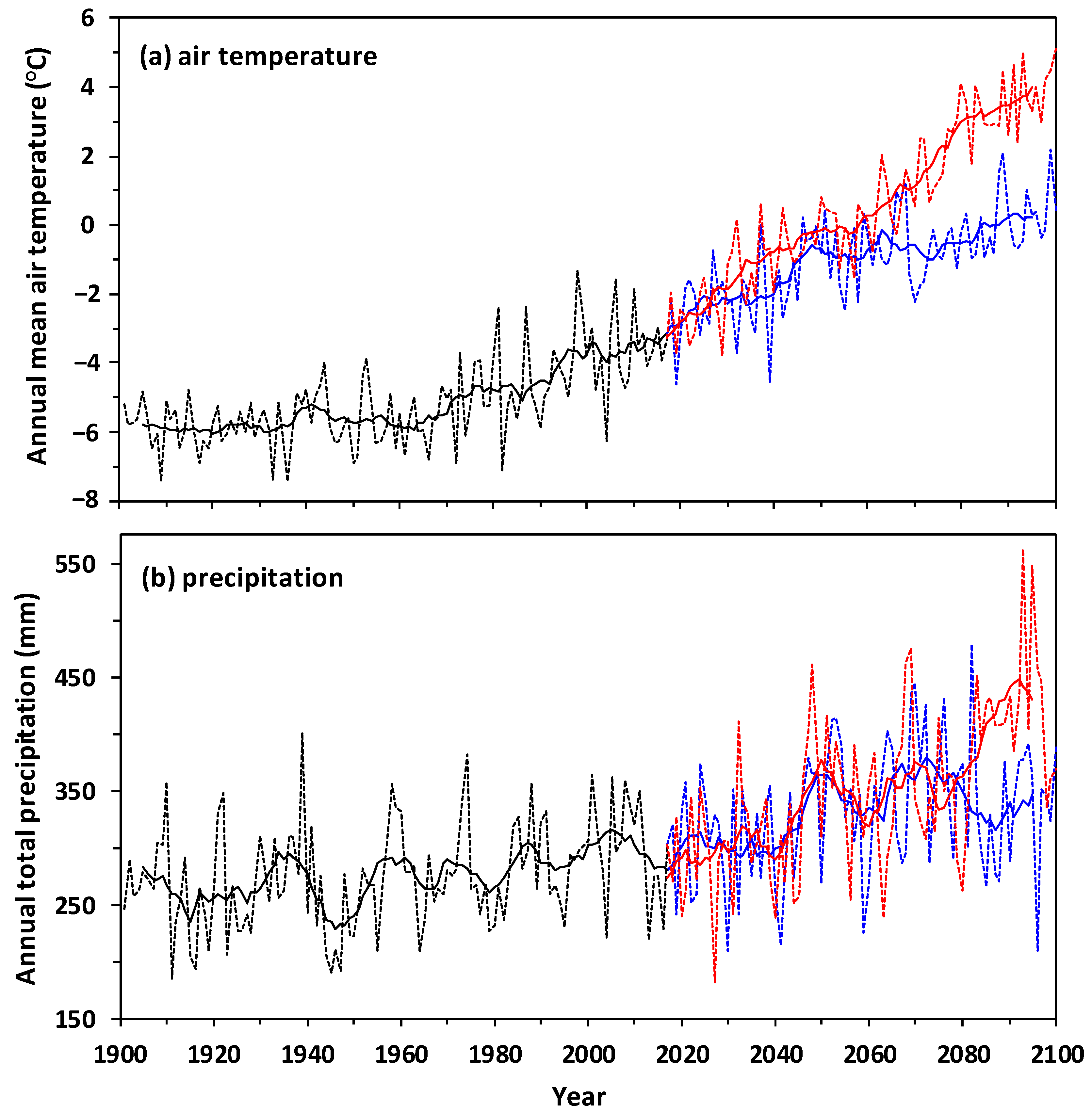
Figure 1 shows an example of air temperature and precipitation time series generated by Met1km for a grid at Yellowknife (62.4540° N, 114.3718° W), depicting both long-term increases and inter-annual fluctuations. From the 1900s (1901–1910) to the 2000s (2001–2010), air temperature increased 2.0 °C and precipitation increased 11.4%. From the 2000s to the 2090s (2091–2100), air temperature is predicted to increase by 4.0 and 7.8 °C under the RCP 4.5 and 8.5 scenarios, respectively. Precipitation is predicted to increase by 9.8% and 36.2%, respectively, under these two scenarios. Daily minimum and maximum air temperatures show similar patterns as that of daily mean air temperature, but the increase in daily minimum air temperature is about 1 °C more than that of the daily maximum air temperature. Vapor pressure and downward longwave radiation also show similar increasing trends as air temperature. Long-term changes are small for wind speed and solar radiation.
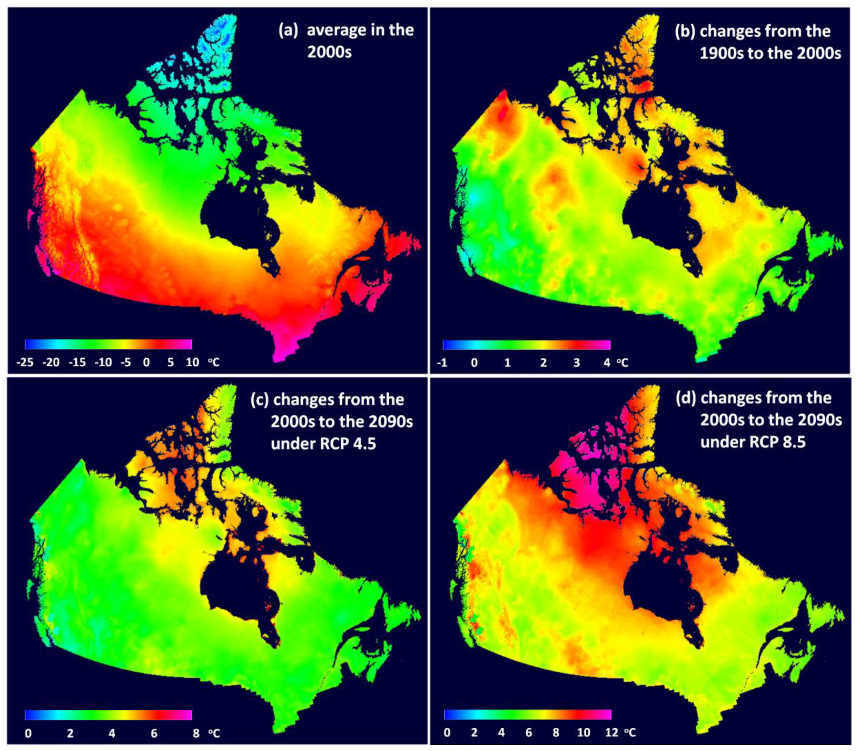
Figure 2a shows the spatial distribution of mean air temperature in the 2000s. Mean air temperature ranges from −25 to 11 °C from the high Arctic to southern Canada. Mean annual air temperature can differ by several degrees in short distances due to variations in topography, especially in British Columbia and high arctic regions. This indicates that it is necessary to develop meteorological datasets at high spatial resolutions. From the 1900s to the 2000s, air temperature increased 1 to 2 °C in southern Canada and 2 to 3 °C in most of northern Canada (Figure 2b). Under the RCP 4.5 climate change scenario, air temperature is predicted to increase by 3 to 4 °C in southern Canada and by 4 to 7 °C in most of northern Canada (Figure 2c). Under the RCP 8.5 scenario, the air temperature is predicted to increase by 5 to 8 °C in most of southern Canada and by 7 to 11 °C in northern Canada, especially in the northwestern Arctic (Figure 2d). These spatial patterns and the magnitudes of future changes are similar to that of the multi-model ensembles from the fifth phase of the Coupled Model Intercomparison Project (CMIP5) for Canadian domain [55].
4.2. Testing the Re-Baselining Spatial Downscaling Method
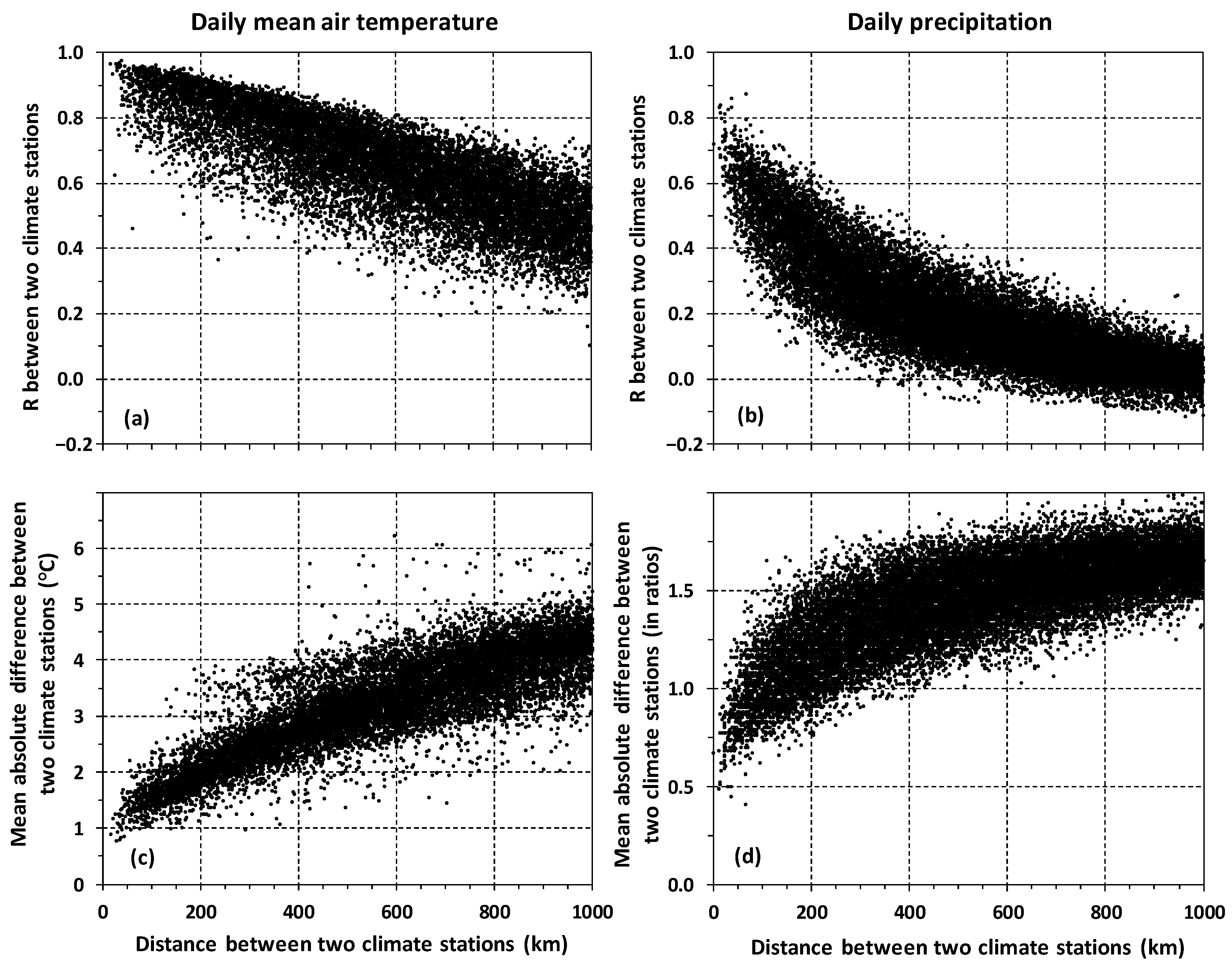
We tested the re-baselining method using the second generation homogenized daily air temperature and precipitation data in Canada [43]. The dataset includes 338 and 463 stations across Canada for air temperature and precipitation, respectively. To test whether a climate variable co-varies at two sites, we calculated R between each pair of climate stations with distance less than 1000 km. To avoid the effects of seasonality, we calculated R using the deviations (using difference for air temperature and ratio for precipitation) from the long-term seasonal patterns, which were linearly interpolated from the long-term monthly averages. We used data from 1945 so that the number of years of the data used for the calculation was similar across the country. The calculated R for air temperature is generally higher than that of precipitation (Figure 3a,b). R decreases with distance between the stations for both air temperature and precipitation, with a near-linear decrease with distance for air temperature but a more rapid initial decrease for precipitation.
To test whether the magnitudes of co-variation are similar at two sites, we calculated the mean absolute difference between each pair of stations using the daily deviations from the long-term average seasonal patterns (using differences for air temperature and ratios for precipitation). The mean absolute difference is the third term in Equation (13), and it is also the MAE of the re-baselining method when using the deviations of one station to estimate another station. The mean absolute differences increase with distance for both air temperature and precipitation, with a near-linear increase with distance for air temperature but a more rapid initial increase for precipitation. These patterns somewhat mirror that of the R (Figure 3c,d). These results indicate that a climate variable (daily air temperature or precipitation) co-varies, and the magnitudes of variations are similar at two stations when their distance is not too far. The co-variation is more consistent for air temperature than for precipitation.
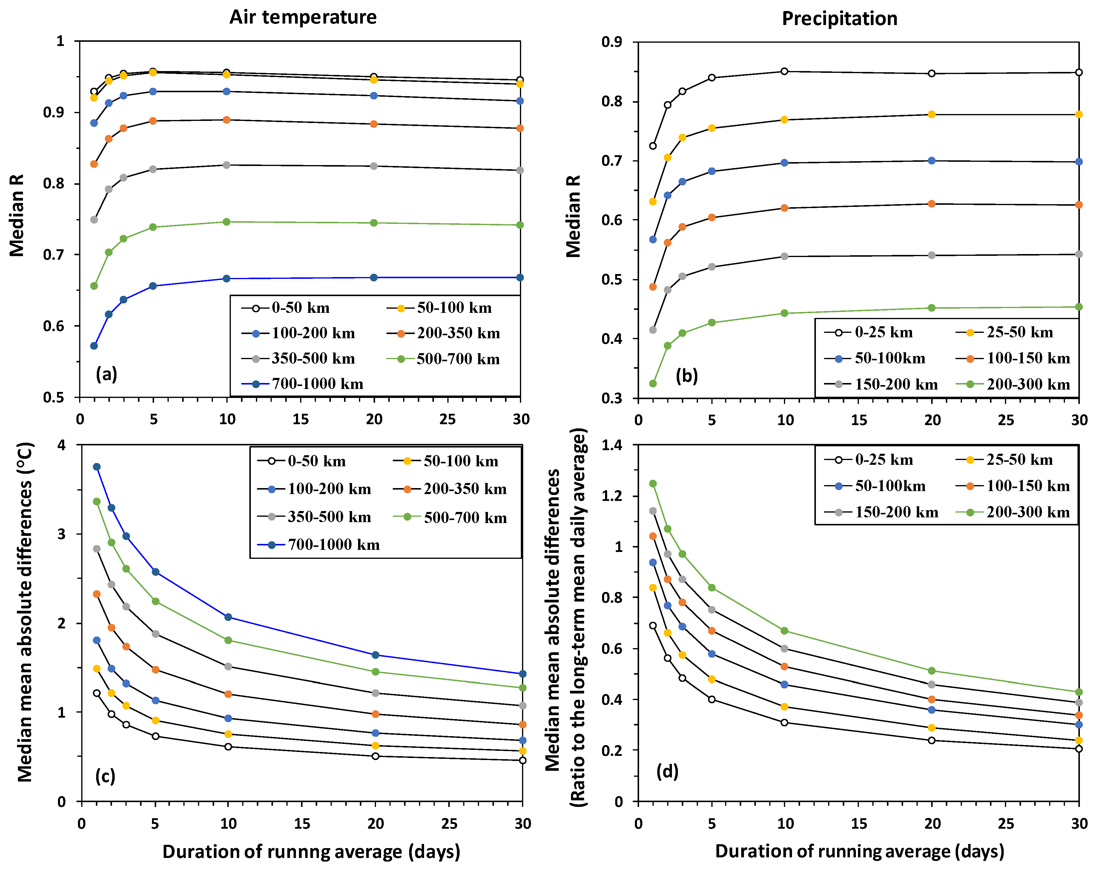
For each pair of stations, we also calculated the R and mean absolute differences using running averages over some days (Figure 4). Each curve in Figure 4 represents the median values of all the pair of stations within a certain range of distances. The median R increases quickly with the duration of the running average from 1 day to about 5–10 days. The increase of R becomes very small when the duration of the running average is longer than 10 days (Figure 4b). Similarly, the median mean absolute difference decreases quickly with the duration of the running average from 1 day to about 5–10 days, then the decrease becomes smaller, especially when two stations are relatively close. This is important because the original re-baselining method was developed and tested based on monthly air temperature [54]. Our tests show that the errors for daily air temperature and precipitation are about 2.5 and 2.9–3.5 times, respectively, of the errors when the re-baselining is calculated using monthly means. The errors decreased rapidly when averaged for some days. The errors for 5- to 10-day averages are not significantly higher than the error calculated using monthly averages. For stations with distances less than 50 km, the median error for 10-day average air temperature is 0.6 °C. For precipitation, the median errors for 10-day averages are 31% and 37% of the long-term averages for distances <25 km and 25–50 km, respectively. Figure 3 and Figure 4 also show that the spatial downscaling errors are smaller when stations are more densely distributed (or the gridded dataset has a higher spatial resolution). Therefore, we generally chose source datasets with high spatial resolutions.
4.3. Comparing Met1km with Climate Station Observations
We compared Met1km with observations at some climate stations across Canada. Although most of the station observations probably were used to develop the gridded source datasets, such comparisons are useful to detect any technical errors and to assess the accuracy of the re-baselining downscaling method. Station data of daily minimum and maximum air temperatures, vapor pressure, wind speed, and solar radiation were derived from hourly data of CWEEDS [44]. Daily station precipitation data were from Environment and Climate Change Canada.
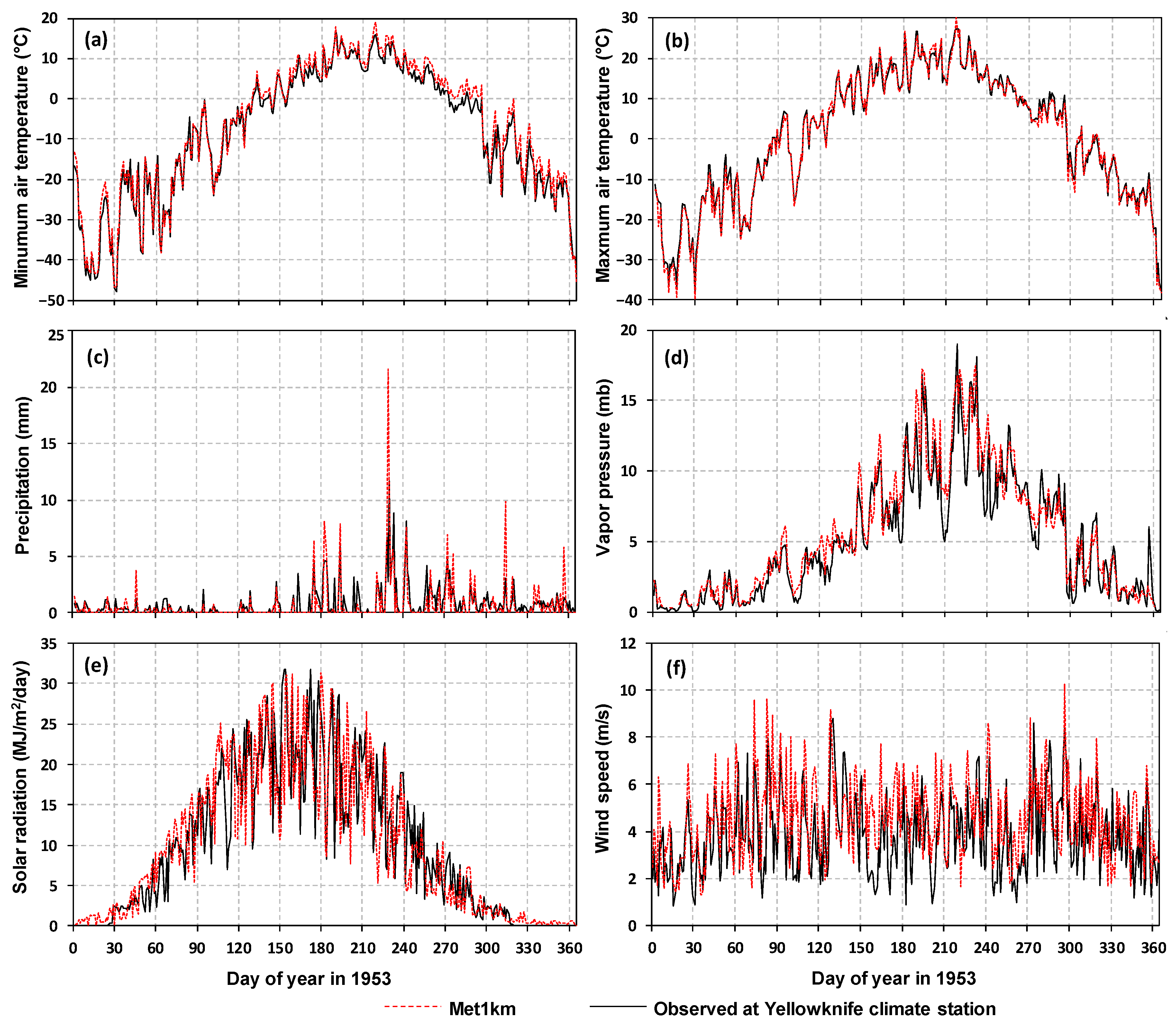
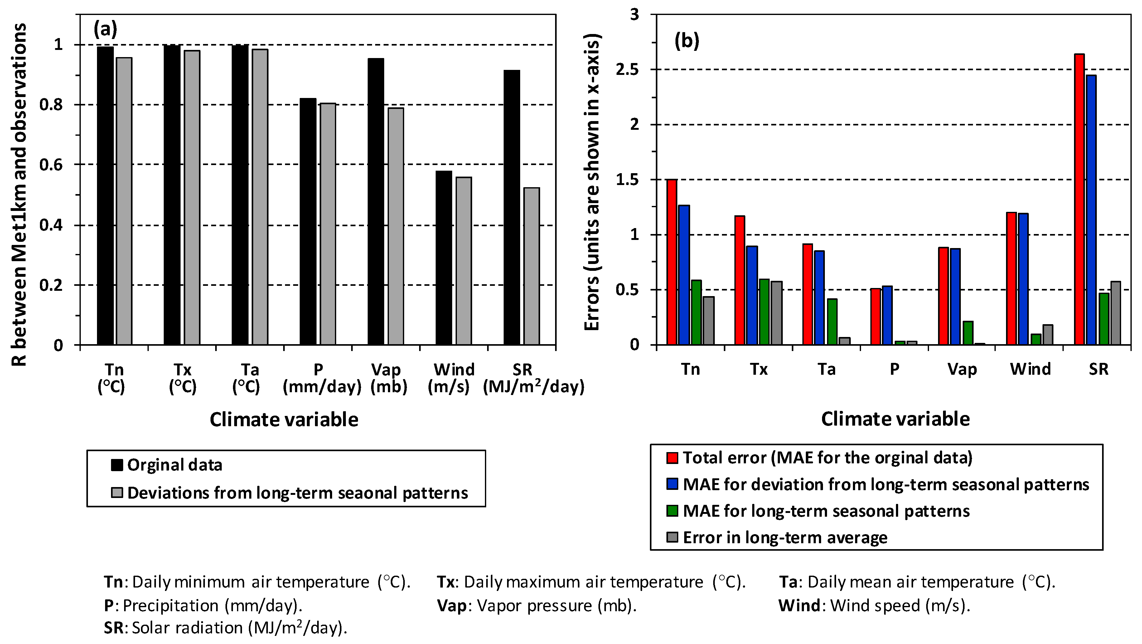
Figure 5 shows some examples of comparison between Met1km and observed climate variables at the Yellowknife airport climate station for the year 1953. Met1km daily values are very close to the observations. Figure 6a shows the R between Met1km and observed daily values from 1948 to 2016 for precipitation and from 1953 to 2005 for other variables. The R is very high for daily minimum, maximum, and mean air temperatures, vapor pressure, and solar radiation. The R is lower for precipitation and wind speed. Since strong seasonal variation could contribute to the high correlations, we also calculated the R after excluding the long-term average seasonal patterns. The long-term average seasonal patterns were calculated by linearly interpolating the long-term monthly averages. The R is still very high for daily minimum, maximum, and mean air temperatures (grey bars in Figure 6a). The R becomes lower for vapor pressure and solar radiation, indicating that Met1km captured their seasonal patterns but the day-to-day fluctuation was not well captured as for air temperatures. The R calculated from the original data and from the deviations are very similar for precipitation and wind speed.
Figure 6b shows the overall error and the three error components for each climate variable for the grid covering the Yellowknife airport climate station. The total error for daily mean air temperature is smaller than that of the daily minimum and maximum air temperatures. The error in daily deviations from the long-term average seasonal patterns are the major sources of the error for all the variables, especially for precipitation, vapor pressure, wind speed, and solar radiation. The errors in long-term averages are very small for daily mean air temperature, precipitation, and vapor pressure. For other variables, the errors in long-term averages are similar to that of the long-term average seasonal patterns. Although the errors in long-term averages are relatively large for daily minimum and maximum air temperatures, the error in long-term average is small for daily mean air temperature.
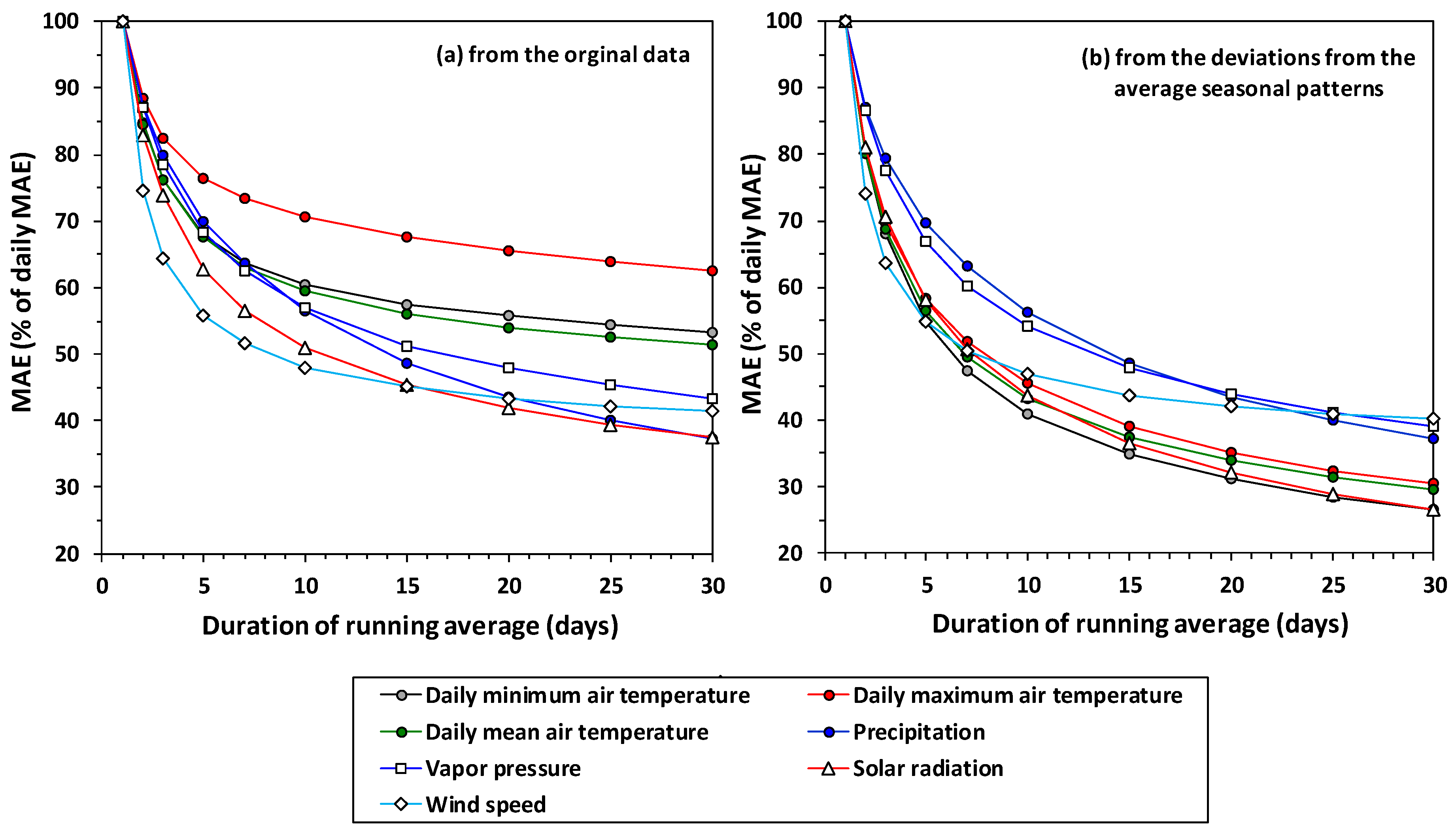
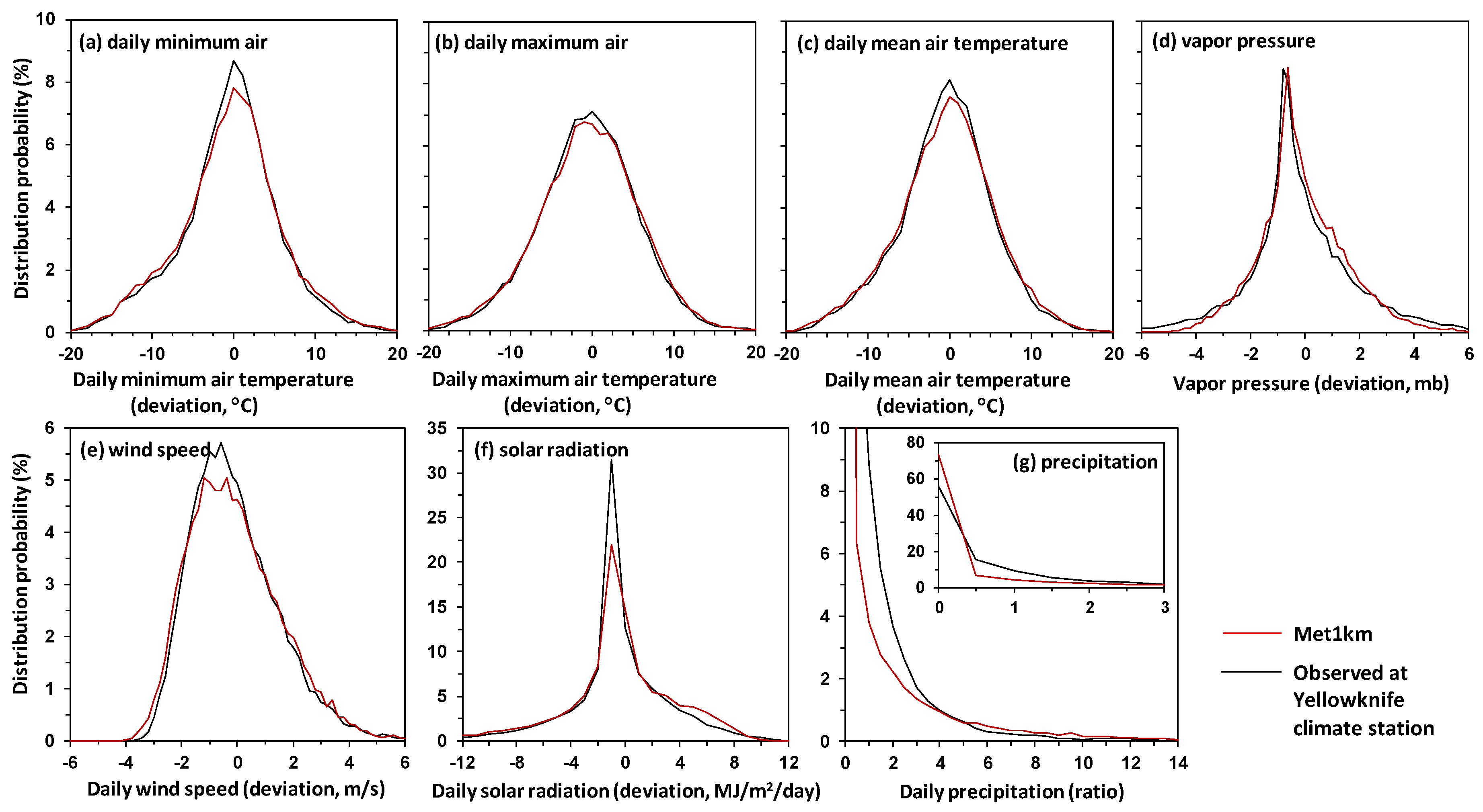
Figure 7 shows the changes in errors with the duration of running average for the Yellowknife airport climate station. The MAE decreased quickly with the duration of running average. When averaged over 10 days, the MAE is about 50 to 60% of the daily errors except daily maximum air temperature, which is about 70% of the daily error. The reduction of MAE is small when the duration of running average is longer than 10 days (Figure 7a). For the deviations from the long-term average seasonal patterns, the reduction of MAE with duration of the running average is even more significant (Figure 7b). In addition, the probability distributions of Met1km are very similar to that of the observations for all the climate variables (Figure 8).
4.4. Comparing with the Homogenized Daily Air Temperature and Precipitation Station Data
We compared Met1km with the second-generation homogenized climate dataset [43] for each station. Because the CRU JRA dataset from 1901 to 1957 was developed by randomly selecting a year between 1958 and 1967 in JRA-55 dataset that is in alignment with the CRU monthly data, the daily errors decreased sharply by about a half from 1 January 1958. Therefore, we did the comparisons separately for the periods from 1901 to 1944 (from 1901 to 1947 in eastern Canada (east of 101° W)) and from 1945 to 2014 (from 1947 to 2014 in eastern Canada).
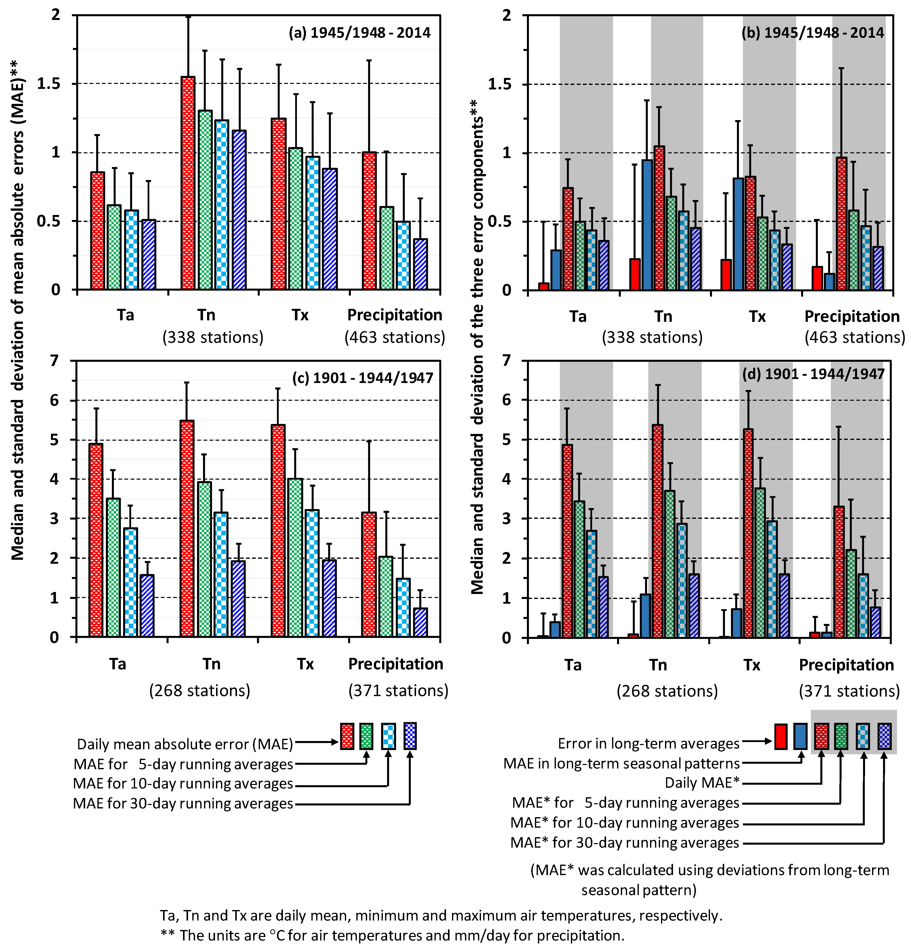
Figure 9a–c shows the median MAE of all the stations for the two periods, respectively. For daily values, the median MAE from 1901 to 1944 is 3 to 5 times of that from 1945 to 2014. The MAE decreases when the climate variables are averaged for a number of days, and the decrease for precipitation is faster than for air temperatures (daily minimum, maximum, and mean), especially for the period from 1901 to 1944. When averaged for 30 days, the MAE from 1901 to 1944 is about twice of that from 1945 to 2014 (1.6, 2.0, 2.7, and 1.8 times for minimum, maximum, and mean air temperatures, and precipitation, respectively). The MAE for daily mean air temperature is smaller than that of daily minimum and maximum air temperatures, especially from 1945 to 2014. Met1km and the climate station data are highly correlated for most of the stations with a linear slope close to 1 from 1945 to 2014. This is even the case when the seasonal patterns are eliminated. However, from 1901 to 1944, the correlations between the daily values of Met1km and the climate station observations are very low after eliminating the average seasonal patterns. The correlation increases when the daily values are averaged over more days, and the correlation reaches a similar level of the correlation during 1945–2014 when the daily values are averaged over 30 days.
Figure 9b–d shows the median values of the three error components of all the stations for the two periods. From 1945 to 2014, the errors in long-term averages are small for temperatures (daily minimum, maximum and mean) and precipitation, as are the errors in average seasonal patterns for daily mean air temperature and precipitation (Figure 9b). The major error for daily mean air temperature and precipitation is in day-to-day fluctuations. For daily minimum and maximum air temperatures, the errors in average seasonal patterns and in day-to-day fluctuations are similar. The errors in day-to-day fluctuations decrease quickly when averaged for 5 to 10 days, and further reduced when averaged in 30 days (Figure 9b). From 1901 to 1944, the errors in long-term averages are very small, as are daily mean air temperature and precipitation. The errors in long-term seasonal patterns for daily minimum and maximum air temperatures are slightly larger. The major sources of the errors are from day-to-day fluctuations. The errors in day-to-day fluctuations decrease quickly and continuously when averaged up to 30 days (Figure 9d).
4.5. Comparing with a Gridded Monthly Anomaly Time-Series Dataset
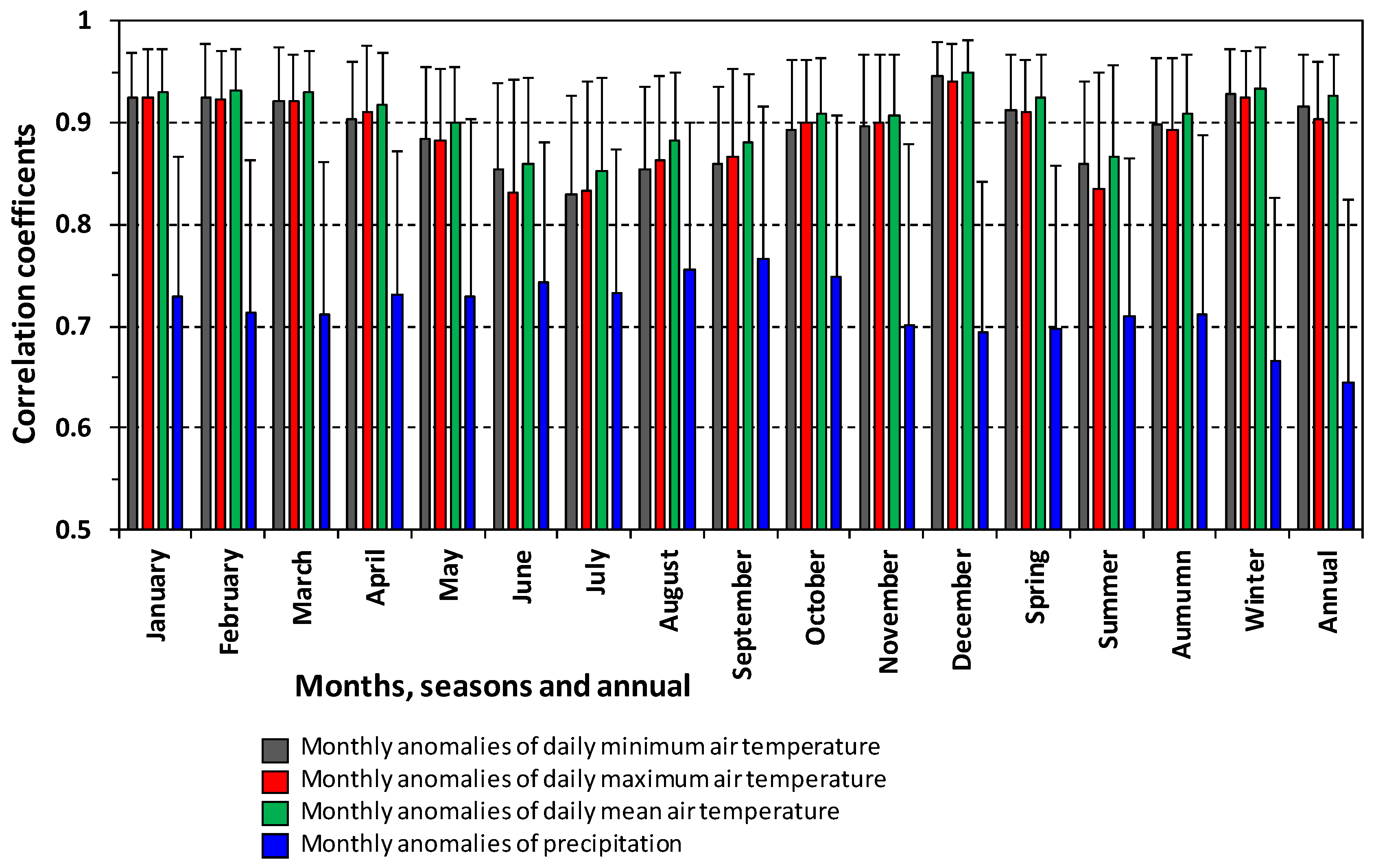
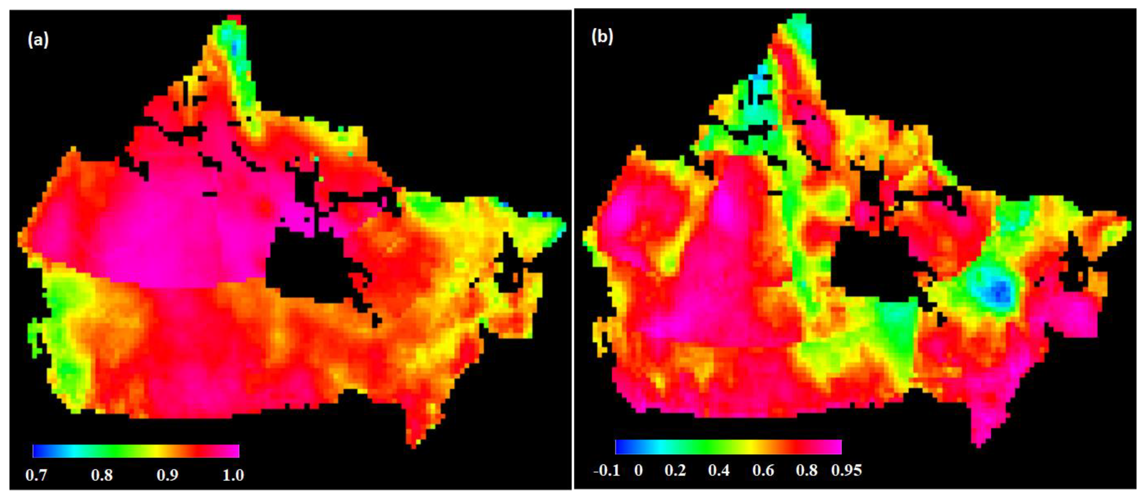
Figure 10 shows the correlation coefficients between CANGRD and monthly anomaly calculated from Met1km. The R is very high for air temperatures (daily minimum, maximum, and mean). The R for the monthly anomalies of daily mean air temperature is slightly higher than that of daily minimum and maximum air temperatures in all the months, seasons, and annual averages. The R for precipitation is much lower than that of air temperatures and the R has a large standard deviation. Figure 11a shows the spatial distribution of R for the anomaly of annual mean air temperature. The sudden increase in R crossing latitude 60° N is due to differences in data length (the data are from 1948 in the north and from 1901 in the south). The R is lower in British Columbia and the eastern high Arctic, probably because of the complex topography in these regions. There is no obvious difference in R between the domain of PNWNAmet and the other areas for air temperature. The R for precipitation is lower than that of air temperatures and has a wider range of variation (Figure 10). R tends to be higher in western Canada (Figure 11b), indicating that the PNWNAmet has a higher accuracy than that of the NRCANmet dataset for precipitation. The correlation is very poor in one area in central Quebec. A close check of the data shows that the discrepancy occurs after 1992, which has an unusually large variation. The downscaled precipitation from the CRU JRA, Princeton and NRCANmet datasets all has a similar pattern for this area, probably because they used the same dataset, which is different from that deriving the CANGRD dataset. The slopes of the linear regressions are close to 1, indicating the fluctuation ranges of CANGRD and Met1km are similar. This comparison indicates that the temporal variation patterns of Met1km are similar to that of the CANGRD dataset.
4.6. Comparing the Accuracy of Met1km and the Source Datasets
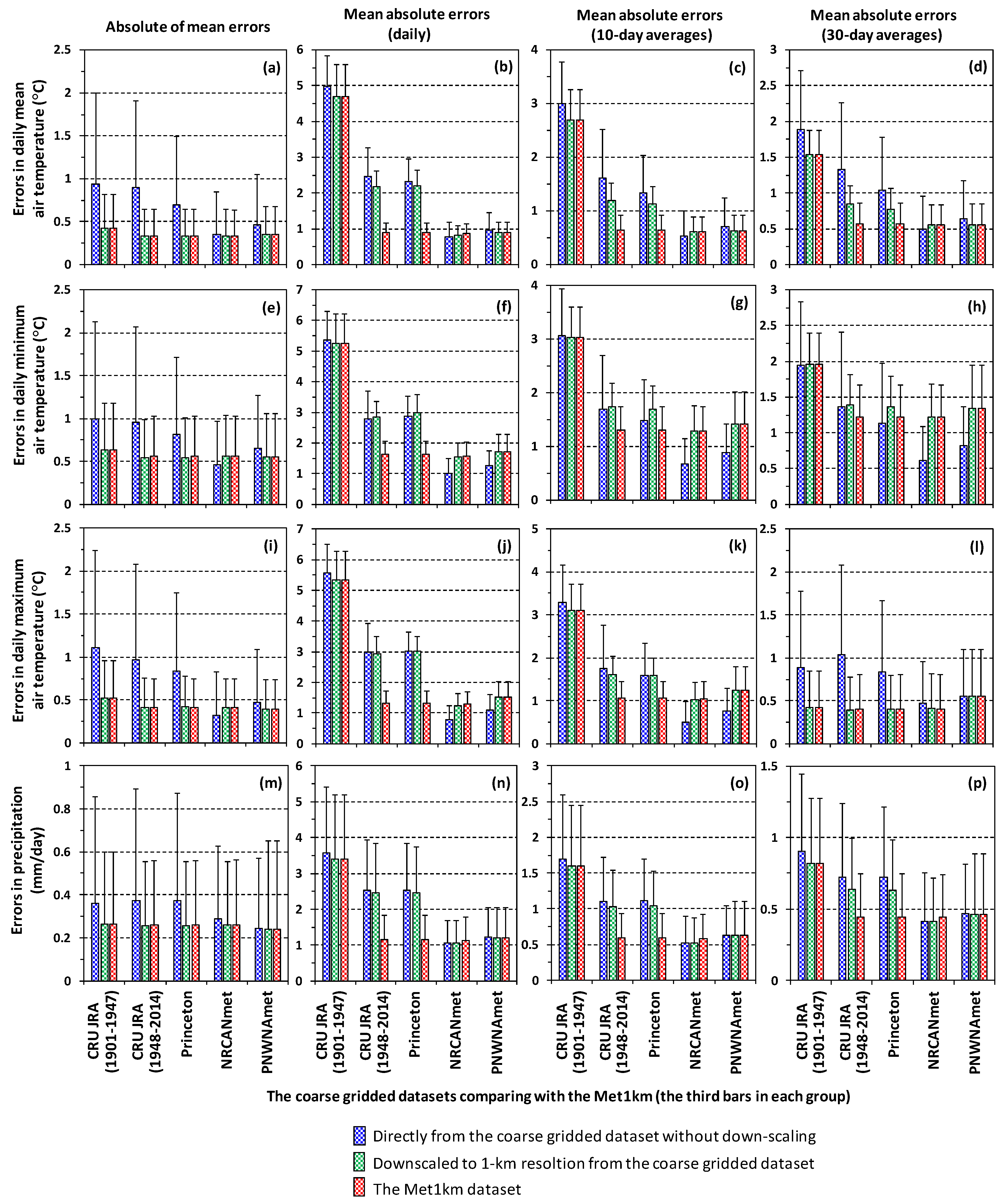
Figure 12 shows the errors of Met1km and the source datasets and the effects of downscaling by comparing with the second generation homogenized daily air temperature and precipitation dataset [43]. The errors of the source datasets were calculated by directly comparing the grid values with the station data. The downscaling effects on the errors were calculated by comparing the station data with the source data downscaled to 1-km resolution using the re-baselining method. For the CRU JRA and the Princeton datasets, spatial downscaling reduced the mean error (absolute value of the error in long-term average) by about a half for daily mean, minimum, and maximum air temperatures, and by about 30% for precipitation. Downscaling also significantly reduced the standard deviation of the mean errors for these two datasets. For daily mean, minimum, and maximum air temperatures, the mean errors of the CRU JRA dataset in 1948–2014 are slightly smaller than that in 1901–1947, and the mean errors are even smaller for the Princeton dataset. The mean errors of precipitation are similar for the CRU JRA dataset in 1901–1947 and 1948–2014, and for the Princeton dataset. For the NRCANmet and PNWNAmet datasets, the effects of downscaling on the mean errors were small and mixed. However, downscaling reduced the standard deviation of the mean errors for air temperatures, especially for the daily means.
Downscaling slightly reduced the MAE for daily air temperature and precipitation for the CRU JRA and Princeton datasets. The daily MAE from 1901 to 1947 is larger than the later period because the data for this period was estimated using an analogy method based on the JRA-55 from 1958 to 1967 and the CRU monthly data [36]. The MAE from 1901 to 1947 decreased quickly when the data were averaged for some days, and the MAE became close to that of CRU JRA in 1948–2014 when averaged for 30 days, especially for daily maximum air temperature. The MAE also reduced for other datasets when the data were averaged for some days. The MAE of the Princeton dataset is slightly smaller than that of CRU JRA in 1948–2014 for daily mean air temperature, but their MAE is similar for daily minimum and maximum air temperatures and precipitation. The MAE of the NRCANmet and PNWNAmet datasets is smaller than that of the CRU JRA and Princeton datasets because the NRCANmet and PNWNAmet datasets were directly interpolated from the climate station data and have fine spatial resolutions. For the NRCANmet and PNWNAmet datasets, downscaling slightly increased the MAE for daily minimum and maximum air temperatures. However, downscaling slightly reduced MAE of daily mean air temperature for the PNWNAmet and reduced the standard deviation of MAE of daily mean air temperature for both the NRCANmet and PNWNAmet datasets. That means downscaling reduced the errors in daily mean air temperature and made it spatially more consistent. The effects of downscaling on precipitation were small for both the NRCANmet and PNWNAmet datasets.
Figure 12 shows that the PNWNAmet dataset had slightly larger errors than that of the NRCANmet dataset. However, their spatial domains were different. For the spatial domain of PNWNAmet, where most of the area is mountainous, the errors of NRCANmet and PNWNAmet were similar but the standard deviation of the errors of PNWNAmet was smaller than that of the NRCANmet, probably because the spatial resolution of PNWNAmet is finer than that of NRCANmet.
5. Discussion
This study developed a long-term (from 1901 to 2100), high-resolution (1 km) daily near-surface meteorological dataset in Canada. Met1km has several advantageous features compared to existing meteorological datasets (Table A1).
It has a high spatial resolution and covers a long-time period at a daily time step for the entire Canadian landmass. It can therefore be used to model long-term dynamics of permafrost and ground thermal conditions at high spatial resolutions. The dataset can also be used for other national-scale modeling and climate impact analysis.
Met1km includes eight climate variables and they are generally consistent in related atmospheric physical processes as they are generated directly from observations or from climate model reanalysis. Therefore, the dataset can be used to drive process-based models and to integrate the effects of these variables through energy and water dynamics.
The dataset is relatively small and flexible to use. Instead of saving the 1-km resolution data for each grid, we developed two scripts to generate spatial and time series data as needed. This treatment significantly reduces the volume of the dataset.
Met1km integrates deemed suitable datasets presently available in term of temporal coverages, spatial resolutions, and data availability. Met1km can be updated easily when better source datasets become available.
The method to generate Met1km for Canada can be used to develop similar datasets for other regions or even to cover the global landmass as the WorldClim2, CRU JRA and Princeton datasets have global coverage.
Comparing to the 1-km daily time series dataset Daymet [19], Met1km integrates more datasets, especially those developed for Canadian domain, and covers a longer time period. The WorldClim2 dataset [29] that we used for re-baselining includes some remote sensing products, which would be very useful to improve the accuracy in high arctic, where climate stations are sparsely distributed [56]. Therefore, Met1km is more suitable for modeling permafrost in Canada. The software toolkit, GlobSim [21], is very useful to improve the applications of climate reanalysis data. However, reanalysis datasets usually have some biases [21,22]. Re-baselining method is very useful to reduce the long-term mean errors (Figure 12). Met1km can be updated to integrate some of the reanalysis datasets, such as the version 5 of the European Centre for Medium-Range Weather Forecasts Re-Analysis (ERA5), if they are deemed better than the ones we used now.
Our tests show that the re-baselining method is useful for spatial downscaling of meteorological data, especially for downscaling coarse gridded datasets. Way and Bonnaventure [54] tested the method for monthly air temperature in northeastern Canada. Our assessment suggests that the method is useful for precipitation as well when distance between two stations is less than 50 km or the resolution of gridded datasets is finer than 0.5° latitude/longitude. The accuracy in 5- to 10-day averages are similar to that of the monthly averages. As precipitation is usually more spatially variable than other climate variables, the re-baselining method may be useful for other climate variables as well. Karger et al. [57] used a similar approach to downscale the 0.5° latitude/longitude CRU monthly air temperature and precipitation to about 1-km resolution. A similar approach was used in three areas in Canada, where the monthly baseline data were from spatially interpolated gridded data (long-term monthly averages) while the daily anomalies were from climate station observations [15,16,17]. Verdin et al. [56] also used a similar method to develop a 5-km resolution daily air temperature dataset by combining 5-km resolution monthly maximum air temperature and the ERA5 dataset. Verdin et al. [56] demonstrate that remotely sensed temperature estimates may more closely represent true conditions than those that rely on interpolation, especially in regions with sparse in situ data.
Our assessments show that the accuracy of Met1km is similar to or better than other gridded datasets (Section 4.6). Our analysis indicates that the major source of errors is due to day-to-day fluctuations. When averaged over 5–10 days, the error is reduced significantly. Since permafrost is not very sensitive to short-term fluctuations in meteorological conditions [43], the effects of short-term errors on modeled permafrost conditions will be limited. For the period from 1901 to 1944, the monthly MAE is about twice of that of 1945–2017. The MAE for daily values is 3–5 times of that of 1945–2017 because the daily data are estimated using an analogy approach [36]. Therefore, the data at the sub-monthly scale is not very reliable for this period. In addition, we used NRCANmet and PNWNAmet datasets to replace air temperature and precipitation because they better mimicked station observations than the CRU JRA and the Princeton datasets (Section 4.6). However, such replacement could cause some inconsistency with other climate variables.
We assessed the accuracy of Met1km mainly by comparing with station observations. Such assessments have some limitations. First, most of the climate station observations may have been used to generate the source datasets. Thus, the observations used for validating Met1km are not completely independent. Second, climate stations are sparsely distributed in northern Canada. The accuracy of the source datasets and thus the generated Met1km dataset can be low in this region due to lack of observations. The error is usually larger for precipitation than for air temperatures, especially over a short time (1 to 10 days). Although we compared with the gridded dataset CANGRD, its spatial resolution (50 km) is coarse. We will continue to update Met1km as new and better source datasets are available, especially the periods before the 1940s and for future projections. Several studies extended the dataset to the beginning of the 20th century (Table A1), and the Twentieth Century Reanalysis project even dated back to middle of the 19th century [58]. These datasets may be useful to improve the accuracy of the data before 1944 and even to extend Met1km back to the end of the Little Ice Age.
6. Conclusions
This study developed a long-term, 1-km resolution daily meteorological dataset in Canada. The dataset includes eight climate variables; therefore, it can be used to drive process-based models for high resolution permafrost modeling and mapping. It can also be used for other land-surface modeling and climate impact studies in Canada.
Met1km dataset is generated based on four coarser gridded meteorological datasets for the historical period: CRU JRA, PNWNAmet, NRCANmet, and the Princeton dataset. The future climate scenarios are from the output of a new Canadian regional climate model under medium-low and high emission scenarios (RCP 4.5 and 8.5). These datasets were downscaled to 1-km resolution using the re-baselining method based on the WorldClim2 dataset as spatial templates. The future scenarios were bias-corrected before re-baselining to 1-km resolution. The accuracy of Met1km is similar to or better than those of the coarse gridded source datasets. The errors in long-term averages and average seasonal patterns are small. The error mainly occurs in day-to-day fluctuations, which decreases quickly when averaged over 5 to 10 days. The error in daily values is large for the period 1901–1944 because the source dataset CRU JRA is developed using an analogy approach based on monthly values. The Met1km, as a data generating system, is relatively small comparing to the total data volume of the 1-km daily time series in Canada, flexible to use for generating spatial and time-series data for applications, and easy to update when new or improved source datasets are available. The methodology of this study can also be used to develop similar datasets for other regions, even the global landmass as most of the source data are in global coverage.
Author Contributions
Conceived the idea and designed the work together, Y.Z. and B.Q.; selected the future scenarios, conducted bias correction, and wrote the related sections, B.Q.; organized the data, assessed the accuracy, and wrote the early version of the manuscript with the input from B.Q. about future climate scenarios, Y.Z.; processed some of the spatial data for accuracy assessment, G.H. All authors discussed the results and contributed to the final manuscript. All authors have read and agreed to the published version of the manuscript.
Funding
This work was funded by “Earth Observation Baseline Data for Cumulative Effects” project in Natural Resources Canada and “Sustainable crop production in Canada under climate change” project in Agriculture and Agri-Food Canada. This study also contributes to NSERC PermafrostNET and a project affiliated to the Arctic Boreal Vulnerability Experiment (ABoVE), a NASA Terrestrial Ecology program.
Acknowledgments
We thank Benita Tam and Sarah Luce in Environment and Climate Change Canada and Daniel McKenney and colleagues in Canadian Forest Service for their advice and data support for this work. We also thank Brendan O’Neill and three anonymous referees reviewing the manuscript. Their comments and suggestions greatly improved the quality of the paper.
Conflicts of Interest
The authors declare no conflict of interest.
Appendix A

Table A1.
A list of the gridded historical meteorological datasets covering Canada (Pure model reanalysis data are not included except for the datasets that cover the periods before the 1940s).
Table A1.
A list of the gridded historical meteorological datasets covering Canada (Pure model reanalysis data are not included except for the datasets that cover the periods before the 1940s).
| Dataset Name | Spatial Coverage | Spatial Resolution | Time Period | Climate Variables * | Methods and References |
|---|---|---|---|---|---|
| CANGRD | Canada landmass | 50 km | 1900–2017 (south) 1948–2017 (North) | Monthly anomalies of Tn, Tx, Ta, and P. | Interpolated using the adjusted and homogenized climate station data. |
| NRCAN met dataset | North America landmass | 5 arc minutes (~10 km) | 1901–2013 for monthly, 1950-2013 for daily | Monthly and daily Tn, Tx, Ta, and P. | Interpolated from climate station data [40,59]. |
| ClimateBC/ WNA/NA | North America landmass | 2.5 arc minutes (~5 km) or any point | 1901–2014, and future scenarios | Monthly Tn, Tx, Ta, and P. | Interpolated from climate station data. Software packages were developed [60]. |
| PNWNA met | North western North America | 3.75 arc minutes (~6 km) | 1945–2012 | Daily Tn, Tx, Ta, P, and Wind. | Interpolated based on the adjusted and homogenized station data [41]. |
| WFDEI-GEM-CaPA | Mackenzie River Basin | 0.125° | 1979–2100 | 3-hourly T, P, Pa, SR, LwR, SH, and Wind. | Blended three datasets together [61]. |
| CHIRTS-daily | 60° S-70° N global land | 0.05° (~5 km) | 1983–2016 | Daily Tn and Tx. | Combined satellite infrared product, station observation, and ERA5 [56]. |
| BEST | Global land and oceans | 0.25° for the U.S.A. and Europe, 1° global | 1701–recent (monthly) 1880–recent (daily) | Monthly and experimental for daily Tn, Tx, and P. | Interpolated based on 5000–7000 climate station data [62]. |
| CRU datasets | Global landmass | 0.5° | 1901–2014 | Monthly Ta, dT, P, WetD, Vap, and Cloud. | Interpolated based on climate station data [37]. |
| CHELSA, CHELSA cruts | Global landmass | 30 arc s (~1 km) | CHELSA: 1979 to 2013, CHELSAcruts: 1901–2016 | Monthly Tn, Tx and P. | CHELSA: down-scaled from the ERA interim reanalysis data. CHELSAcruts: downscaled from CRU data [57]. |
| WorldClim2 | Global landmass | 30 arc s (~1 km) | Averages in 1970–2000 | Monthly Tn, Tx, Ta, P, SR, Vap, and Wind. | Interpolated based on climate station data and satellite derived covariates [29]. |
| METEO 1KM | Global landmass | 1 km | 2011 | Daily Ta. | Combining climate station data, topographical and satellite images [30,31]. |
| Terra Climate | Global landmass | 2.5 arc m (~4 km) | 1958–2019 | Monthly Tn, Tx, Ta, P, SR, Vap, and Wind. | Combining CRU, WorlClim, and JRA-55 [63]. |
| Princeton dataset | Global landmass | 0.5°(V2) 0.25°(V3) | 1901–2012 (V2) 1948–2016 (V3) | 3-hourly, daily, monthly Tn, Tx, Ta, P, SR, LwR, Vap, and Wind. | Combining observation-based datasets with a climate reanalysis dataset [39]. |
| CRU JRA | Global landmass | 0.5° | 1901–2017 | 6-hourly T, P, SH, Pa, Wind, SR and LwR. | Combining CRU data with JRA-55 [36]. |
| WATCH Forcing Data (WFD) | Global landmass | 0.5° | 1901–2001 | 3- or 6-hourly T, P, SH, Pa, SR, LwR, Wind. | ERA-40 for 1958–2001 and re-ordering the ERA-40 for 1901–1957 [64]. |
| WFDEI | Global landmass | 0.5° | 1979–2016 | 3-hourly T, P, SH, Pa, SR, LwR, Wind. | Similar to WED but using ERA-Interim [65]. |
| 20th century reanalysis (20CR) | Global | 2° | 1871–2012 | Multiple variables (6-hourly) from model reanalysis. | Model reanalysis mainly constrained by surface pressure [57,66]. |
| ERA-20C | Global | About 125 km | 1900–2010 | Multiple variables (6-hourly) from model reanalysis. | Model reanalysis constrained by surface pressure and marine wind [67]. |
| Daymet | North America, Puerto Rico, and Hawaii | 1 km | 1980–2017 | Daily Tn, Tx, P, SR, Vap, and Snow. | Interpolated based on climate station data [19]. |
| GlobSim | Global | Any location | Same as the reanalysis datasets | Same as the reanalysis datasets. | A software toolkit to generate time series data for any sites from several reanalysis datasets [21]. |
* T is the mean air temperature for a define period (at sub-daily scales). Ta, Tn, and Tx are daily mean, minimum and maximum air temperatures, respectively, dT is diurnal air temperature range, P is precipitation, Pa is atmospheric pressure, Vap is vapor pressure, SH is specific humidity, WetD is wet-days, Cloud is cloud cover, SR is solar radiation, LwR is downward longwave radiation, Snow is snow water equivalent.
Appendix B
Calculating Monthly Mean Downward Longwave Radiation
We estimated monthly mean downward longwave radiation corresponding to the time scale and spatial resolution of the WorldClim2 dataset (monthly average from 1970 to 2000 at resolution of 30 arc seconds latitude/longitude) [29]. Based on the assessment of different methods conducted by Flerchinger et al. [68], especially the accuracy in cold regions, we estimated downward longwave radiation using the method of Kimball et al. [69] with clear-sky downward longwave radiation estimated by the method of Dilley and O’Brien [70].
where
where L is all sky downward longwave radiation (in W/m2), Lclr is downward longwave radiation for clear sky, c is the fraction of cloud cover, T0 is air temperature observed at about 2 m above the land surface (in K), and Tc is the temperature on the base of the cloud (in K), which is assumed 9 K lower than the T0. σ is the Stefan-Boltzmann constant (5.67 × 10⁻⁸ W/m2/K4), e0 is the vapor pressure observed about 2 m above the surface (in kPa). The equations and parameters are from Flerchinger et al. [69]. We calculated monthly mean downward longwave radiation for each 1-km grid based on the monthly mean air temperature and vapor pressure of the corresponding WorldClim2 grid. As high arctic regions receive very low and even no solar radiation in winter months, we estimated the cloud cover fraction based on CRU TS data [37].
References
- Gruber, S. Derivation and analysis of a high-resolution estimate of global permafrost zonation. Cryosphere 2012, 6, 221–233. [Google Scholar] [CrossRef] [Green Version]
- Zhang, T.; Barry, R.G.; Knowles, K.; Heginbottom, J.A.; Brown, J. Statistics and characteristics of permafrost and ground ice distribution in the Northern Hemisphere. Polar Geogr. 1999, 23, 147–149. [Google Scholar] [CrossRef]
- Biskaborn, B.K.; Smith, S.L.; Noetzli, J.; Matthes, H.; Vieira, G.; Streletskiy, D.A.; Schoeneich, P.; Romanovsky, V.E.; Lewkowicz, A.G.; Abramov, A.; et al. Permafrost is warming at a global scale. Nat. Commun. 2019, 10, 264. [Google Scholar] [CrossRef] [PubMed] [Green Version]
- Frauenfeld, O.W.; Zhang, T.J.; Barry, R.G.; Gilichinsky, D. Interdecadal changes in seasonal freeze and thaw depths in Russia. J. Geophys. Res. 2004, 109, D05101. [Google Scholar] [CrossRef]
- Oberman, N.G. Contemporary Permafrost Degradation of Northern European Russia. In Proceedings of the Ninth International Conference on Permafrost, Fairbanks, AK, USA, 29 June 2008; Kane, D.L., Hinkel, K.M., Eds.; Institute of Northern Engineering, University of Alaska: Fairbanks, AK, USA, 2008; Volume 2, pp. 1305–1310. [Google Scholar]
- Thibault, S.; Payette, S. Recent permafrost degradation in bogs of the James Bay area, northern Quebec, Canada. Permafr. Periglac. Process. 2009, 20, 383. [Google Scholar] [CrossRef]
- James, M.; Lewkowicz, A.G.; Smith, S.L.; Miceli, C.M. Multi-decadal degradation and persistence of permafrost in the Alaska Highway corridor, northwest Canada. Environ. Res. Lett. 2013, 8, 045013. [Google Scholar] [CrossRef]
- Hjort, J.; Karjalainen, O.; Aalto, J.; Westermann, S.; Romanovsky, V.E.; Nelson, F.E.; Etzelmüller, B.; Luoto, M. Degrading permafrost puts Arctic infrastructure at risk by mid-century. Nat. Commun. 2018, 9, 5147. [Google Scholar] [CrossRef]
- Lewkowicz, A.G.; Way, R. Extremes of summer climate trigger thousands of thermokarst landslides in a high arctic environment. Nat. Commun. 2019, 10, 1329. [Google Scholar] [CrossRef] [Green Version]
- Yumashev, D.; Hope, C.; Schaefer, K.; Riemann-Campe, K.; Iglesias-Suarez, F.; Jafarov, E.; Burke, E.J.; Young, P.J.; Elshorbany, Y.; Whiteman, G. Climate policy implications of nonlinear decline of Arctic land permafrost and other cryosphere elements. Nat. Commun. 2019, 10, 1900. [Google Scholar] [CrossRef] [Green Version]
- Obu, J.; Westermann, S.; Bartsch, A.; Berdnikov, N.; Christiansen, H.H.; Dashtseren, A.; Delaloye, R.; Elberling, B.; Etzelmüller, B.; Kholodov, A.; et al. Northern Hemisphere permafrost map based on TTOP modelling for 2000–2016 at 1 km2 scale. Earth-Sci. Rev. 2019, 193, 299–316. [Google Scholar] [CrossRef]
- Karjalainen, O.; Aalto, J.; Luoto, M.; Westermann, S.; Romanovsky, V.E.; Nelson, F.E.; Bernd Etzelmüller, B.; Hjort, J. Circumpolar permafrost maps and geohazard indices for near-future infrastructure risk assessments. Sci. Data 2019, 6, 190037. [Google Scholar] [CrossRef] [PubMed] [Green Version]
- Zhang, Y.; Chen, W.; Riseborough, D.W. Temporal and spatial changes of permafrost in Canada since the end of the Little Ice Age. J. Geophys. Res. 2006, 111, D22103. [Google Scholar] [CrossRef] [Green Version]
- Zhang, Y.; Chen, W.; Riseborough, D.W. Disequilibrium response of permafrost thaw to climate warming in Canada over 1850–2100. Geophys. Res. Lett. 2008, 35, L02502. [Google Scholar] [CrossRef]
- Zhang, Y.; Li, J.; Wang, X.; Chen, W.; Sladen, W.; Dyke, L.; Dredge, L.; Poitevin, J.; McLennan, D.; Stewart, H.; et al. Modelling and mapping permafrost at high spatial resolution in Wapusk National Park, Hudson Bay Lowlands. Can. J. Earth Sci. 2012, 49, 925–937. [Google Scholar] [CrossRef]
- Zhang, Y.; Wang, X.; Fraser, R.; Olthof, I.; Chen, W.; Mclennan, D.; Ponomarenko, S.; Wu, W. Modelling and mapping climate change impacts on permafrost at high spatial resolution for a region with complex terrain. Cryosphere 2012, 7, 1121–1137. [Google Scholar] [CrossRef] [Green Version]
- Zhang, Y.; Wolfe, S.A.; Morse, P.D.; Olthof, I.; Fraser, R.H. Spatiotemporal impacts of wildfire and climate warming on permafrost across a subarctic region, Canada. J. Geophys. Res. Earth Surf. 2015, 120, 2338–2356. [Google Scholar] [CrossRef] [Green Version]
- Aalto, J.; Karjalainen, O.; Hjort, J.; Luoto, M. Statistical forecasting of current and future circum-Arctic ground temperatures and active layer thickness. Geophys. Res. Lett. 2018, 45, 4889–4898. [Google Scholar] [CrossRef] [Green Version]
- Thornton, P.E.; Thornton, M.M.; Mayer, B.W.; Wei, Y.; Devarakonda, R.; Vose, R.S.; Cook, R.B. Daymet: Daily Surface Weather Data on a 1-km Grid for North America, Version 3; ORNL DAAC: Oak Ridge, TN, USA, 2017. [Google Scholar]
- Thornton, P.E.; Running, S.W.; White, M.A. Generating surfaces of daily meteorological variables over large regions of complex terrain. J. Hydrol. 1997, 190, 214–251. [Google Scholar] [CrossRef] [Green Version]
- Cao, B.; Quan, X.; Brown, N.; Stewart-Jones, E.; Gruber, S. GlobSim (v1.0): Deriving meteorological time series for point locations from multiple global reanalyses. Geosci. Model. Dev. 2019, 12, 4661–4679. [Google Scholar] [CrossRef] [Green Version]
- Reeves Eyre, J.E.J.; Zeng, X. Evaluation of greenland near surface air temperature datasets. Cryosphere 2017, 11, 1591–1605. [Google Scholar] [CrossRef] [Green Version]
- Zhang, Y.; Chen, W.; Cihlar, J. A process-based model for quantifying the impact of climate change on permafrost thermal regimes. J. Geophys. Res. 2003, 108, 4695. [Google Scholar]
- Endrizzi, S.; Gruber, S.; Dall’Amico, M.; Rigon, R. GEOtop 2.0: Simulating the combined energy and water balance at and below the land surface accounting for soil freezing, snow cover and terrain effects. Geosci. Model. Dev. 2014, 7, 2831–2857. [Google Scholar] [CrossRef] [Green Version]
- Westermann, S.; Langer, M.; Boike, J.; Heikenfeld, M.; Peter, M.; Etzelmüller, B.; Krinner, G. Simulating the thermal regime and thaw processes of ice-rich permafrost ground with the land-surface model CryoGrid 3. Geosci. Model. Dev. 2016, 9, 523–546. [Google Scholar] [CrossRef] [Green Version]
- Zhang, Y.; Chen, W.; Riseborough, D.W. Modeling the Long-Term Dynamics of Snow and Their Impacts on Permafrost in Canada. In Proceedings of the Ninth International Conference on Permafrost, Fairbanks, AK, USA, 29 June 2008; Kane, D.L., Hinkel, K.M., Eds.; Institute of Northern Engineering, University of Alaska: Fairbanks, AL, USA, 2008; pp. 2055–2060. [Google Scholar]
- Heginbottom, J.A.; Dubreuil, M.A.; Harker, P.T. Canada: Permafrost, National Atlas of Canada, 5th ed.; In MCR 4177; Natural Resources Canada: Ottawa, ON, Canada, 1995.
- Kettles, I.M.; Tarnoca, C.; Bauke, S.D. Predicted permafrost distribution in Canada under a climate warming scenario. In Current Research; Geological Survey of Canada: Ottawa, ON, Canada, 1997; pp. 109–115. [Google Scholar]
- Fick, S.E.; Hijmans, R.J. WorldClim 2: New 1-Km spatial resolution climate surfaces for global land areas. Int. J. Climatol. 2017, 37, 4302–4315. [Google Scholar] [CrossRef]
- Kilibarda, M.; Hengl, T.; Heuvelink, G.; Gräler, B.; Pebesma, E.; Tadić, M.P.; Bajat, B. Spatio-temporal interpolation of daily temperatures for global land areas at 1 km resolution. J. Geophys. Res. 2017, 119, 2294–2313. [Google Scholar] [CrossRef] [Green Version]
- Kilibarda, M.; Tadić, M.P.; Hengl, T.; Luković, J.; Bajat, B. Global geographic and feature space coverage of temperature data in the context of spatio-temporal interpolation. Spat. Stat. 2015, 14, 22–38. [Google Scholar] [CrossRef]
- Nicolsky, D.J.; Romanovsky, V.E.; Panda, S.K.; Marchenko, S.S.; Muskett, R.R. Applicability of the ecosystem type approach to model permafrost dynamics across the Alaska North Slope. J. Geophys. Res. Earth Surf. 2017, 122, 50–75. [Google Scholar] [CrossRef]
- Beltrami, H.; Gosselin, C.; Mareschal, J.C. Ground surface temperatures in Canada: Spatial and temporal variability. Geophys. Res. Lett. 2003, 30, 1499. [Google Scholar] [CrossRef] [Green Version]
- Hinkel, K.M.; Paetzold, F.; Nelson, F.E.; Bockheim, J.G. Patterns of soil temperature and moisture in the active layer and upper permafrost at Barrow, Alaska: 1993–1999. Glob. Planet. Chang. 2001, 29, 293–309. [Google Scholar] [CrossRef]
- Chen, W.; Zhang, Y.; Cihlar, J.; Smith, S.L.; Riseborough, D.W. Changes in soil temperature and active-layer thickness during the 20th century in a region in western Canada. J. Geophys. Res. 2003, 108, 4696. [Google Scholar]
- Harris, I.C. CRU JRA v1.1: A Forcings Dataset of Gridded Land Surface Blend of Climatic Research Unit (CRU) and Japanese Reanalysis (JRA) Data; Jan.1901–Dec.2017; Centre for Environmental Data Analysis: Didcot, UK, 2019. [Google Scholar]
- Harris, I.; Jones, P.D.; Osborn, T.J.; Lister, D.H. Updated high-resolution grids of monthly climatic observations—The CRU TS3.10 Dataset. Int. J. Climatol. 2014, 34, 623–642. [Google Scholar] [CrossRef] [Green Version]
- Kobayashi, S.; Ota, Y.; Harada, Y.; Ebita, A.; Moriya, M.; Onoda, H.; Onogi, K.; Kamahori, H.; Kobayashi, C.; Endo, H.; et al. The JRA-55 reanalysis: General specifications and basic characteristics. J. Met. Soc. Jap. 2015, 93, 5–48. [Google Scholar] [CrossRef] [Green Version]
- Sheffield, J.; Goteti, G.; Wood, E.F. Development of a 50-year high-resolution global dataset of meteorological forcings for land surface modeling. J. Clim. 2006, 19, 3088–3111. [Google Scholar] [CrossRef] [Green Version]
- McKenney, D.W.; Hutchinson, M.F.; Papadopol, P.; Lawrence, K.; Pedlar, J.; Campbell, K.; Milewska, E.; Hopkinson, R.; Price, D.; Owen, T. Customized spatial climate models for North America. B Am. Meteorol. Soc. 2011, 92, 1611–1622. [Google Scholar] [CrossRef]
- Werner, A.T.; Schnorbus, M.A.; Shrestha, R.R.; Cannon, A.J.; Zwiers, F.W.; Dayon, G.; Anslow, F. A long-term, temporally consistent, gridded daily meteorological dataset for northwestern North America. Sci. Data 2019, 6, 180299. [Google Scholar] [CrossRef] [Green Version]
- Scinocca, J.F.; Kharin, V.V.; Jiao, Y.; Qian, M.W.; Lazare, M.; Solheim, L.; Flato, G.M.; Biner, S.; Desgagne, M.; Dugaa, B. Coordinated global and regional climate modeling. J. Clim. 2016, 29, 17–35. [Google Scholar] [CrossRef]
- Vincent, L.A.; Wang, X.L.; Milewska, E.J.; Wan, H.; Yang, F.; Swail, V. A second generation of homogenized Canadian monthly surface air temperature for climate trend analysis. J. Geophys. Res. 2012, 117, D18110. [Google Scholar] [CrossRef]
- Environment Canada and the National Research Council of Canada. Can. Weather Energy Eng. Data Sets (CWEEDS Files) Can. Weather Energy Calc. (CWEC Files); Environment Canada and the National Research Council of Canada: Ottawa, ON, Canada, 2007; Updated User’s Manual.
- IPCC. Climate Change 2013: The Physical Science Basis. Contribution of Working Group I to the Fifth Assessment Report of the Intergovernmental Panel on Climate Change; Stocker, T.F., Qin, D., Plattner, G.-K., Tignor, M., Allen, S.K., Boschung, J., Nauels, A., Xia, Y., Bex, V., Midgley, P.M., Eds.; Cambridge University Press: Cambridge, UK, 2013; p. 1535. [Google Scholar]
- Mearns, L.O.; Arritt, R.; Biner, S.; Bukovsky, M.S.; McGinnis, S.; Sain, S.; Caya, D.; Correia, J., Jr.; Flory, D.; William Gutowski, W.; et al. The North American regional climate change assessment program: Overview of phase I results. Bull. Am. Meteorol. Soc. 2012, 93, 1337–1362. [Google Scholar] [CrossRef]
- Qian, B.; Wang, H.; He, Y.; Liu, J.; De Jong, R. Projecting spring wheat yield changes on the Canadian Prairies: Effects of resolutions of a regional climate model and statistical processing. Int. J. Climatol. 2016, 36, 3492–3506. [Google Scholar] [CrossRef] [Green Version]
- Qian, B.; Jing, Q.; Bélanger, G.; Shang, J.; Huffman, T.; Liu, J.; Hoogenboom, G. Simulated canola yield responses to climate change and adaptation in Canada. J. Agron. 2018, 110, 14. [Google Scholar] [CrossRef] [Green Version]
- He, W.; Yang, J.Y.; Qian, B.; Drury, C.F.; Hoogenboom, G.; He, P.; Lapen, D.; Zhou, W. Climate change impacts on crop yield, soil water balance and nitrate leaching in the semiarid and humid regions of Canada. PLoS ONE 2018, 13, e0207370. [Google Scholar] [CrossRef] [PubMed]
- Christensen, J.H.; Boberg, F.; Christensen, O.B.; Lucas-Picher, P. On the need for bias correction of regional climate change projections of temperature and precipitation. Geophys. Res. Lett. 2008, 35, L20709. [Google Scholar] [CrossRef]
- Iizumi, T.; Yokozawa, M.; Nishimori, M. Probabilistic evaluation of climate change impacts on paddy rice productivity in Japan. Clim. Chang. 2010, 107, 391–415. [Google Scholar] [CrossRef] [Green Version]
- Qian, B.; Gameda, S.; Hayhoe, H.; De Jong, R.; Bootsma, A. Comparison of LARS-WG and AAFC-WG stochastic weather generators for diverse Canadian climates. Clim. Res. 2004, 26, 175–191. [Google Scholar]
- Li, H.; Sheffield, J.; Wood, E.F. Bias correction of monthly precipitation and temperature fields from Intergovernmental Panel on Climate Change AR4 models using equidistanct quantile matching. J. Geophys. Res. 2010, 115, D10101. [Google Scholar] [CrossRef]
- Way, R.G.; Bonnaventure, P.P. Testing a reanalysis-based infilling method for areas with sparse discontinuous air temperature data in northeastern Canada. Atmos. Sci. Lett. 2015, 16, 398–407. [Google Scholar] [CrossRef]
- Zhang, X.; Flato, G.; Kirchmeier-Young, M.; Vincent, L.; Wan, H.; Wang, X.; Rong, R.; Fyfe, J.; Li, G.; Kharin, V.V. Changes in temperature and precipitation across Canada, Chapter 4. In Canada’s Changing Climate Report; Bush, E., Lemmen, D.S., Eds.; Government of Canada: Ottawa, ON, Canada, 2019; pp. 112–193. [Google Scholar]
- Verdin, A.; Funk, F.; Peterson, P.; Landsfeld, M.; Tuholske, C.; Grace, K. Development and validation of the CHIRTS-daily quasi-global high resolution daily temperature data set. Sci. Data 2020, 7, 303. [Google Scholar] [CrossRef]
- Karger, D.N.; Conrad, O.; Böhner, J.; Kawohl, T.; Kreft, H.; Soria-Auza, R.W.; Zimmermann, N.E.; Linder, H.P.; Kessler, M. Climatologies at high resolution for the earth’s land surface areas. Sci. Data 2017, 4, 170122. [Google Scholar] [CrossRef] [Green Version]
- Slivinski, L.C.; Compo, G.P.; Whitaker, J.S.; Sardeshmukh, P.D.; Giese, B.S.; McColl, C.; Allan, R.; Yin, X.; Vose, R.; Titchner, H.; et al. Towards a more reliable historical reanalysis: Improvements for version 3 of the Twentieth Century Reanalysis system. Q. J. R. Meteorol. Soc. 2019, 145, 2876–2908. [Google Scholar] [CrossRef] [Green Version]
- McKenney, D.W.; Pedlar, J.H.; Papadopol, P.; Hutchinson, M.F. The development of 1901–2000 historical monthly climate models for Canada and the United States. Agric. For. Meteorol. 2006, 138, 69–81. [Google Scholar] [CrossRef]
- Wang, A.; Zeng, X. Development of global hourly 0.5-degree land surface air temperature datasets. J. Clim. 2013, 26, 7676–7691. [Google Scholar] [CrossRef]
- Asong, Z.E.; Elshamy, M.E.; Princz, D.; Wheater, H.S.; Pomeroy, J.W.; Pietroniro, A.; Cannon, A. High-resolution meteorological forcing data for hydrological modelling and climate change impact analysis in the Mackenzie River Basin. Earth Syst. Sci. Data 2020, 12, 629–645. [Google Scholar] [CrossRef] [Green Version]
- Rohde, R.; Muller, R.A.; Jacobsen, R.; Muller, E.; Perlmutter, S.; Rosenfeld, A.; Wurtele, J.; Groom, D.; Wickham, C. A new estimate of the average earth surface land temperature spanning 1753 to 2011. Geoinf. Geostat. Overv. 2013, 1, 1. [Google Scholar]
- Abatzoglou, J.; Dobrowski, S.Z.; Parks, S.A.; Hegewisch, K.C. TerraClimate, a high-resolution global dataset of monthly climate and climatic water balance from 1958–2015. Sci. Data 2018, 5, 170191. [Google Scholar] [CrossRef] [PubMed] [Green Version]
- Weedon, G.P.; Gomes, S.; Viterbo, P.; Shuttleworth, W.J.; Blyth, E.; Osterle, H.; Adam, J.C.; Bellouin, N.; Boucher, O.; Best, M. Creation of the WATCH forcing data and its use to assess global and regional reference crop evaporation over land during the twentieth century. J. Hydrometeorol. 2011, 12, 823–848. [Google Scholar] [CrossRef] [Green Version]
- Weedon, G.P.; Balsamo, G.; Bellouin, N.; Gomes, S.; Best, M.J.; Viterbo, P. The WFDEI meteorological forcing data set: WATCH Forcing Data methodology applied to ERA-Interim reanalysis data. Water Resour. Res. 2014, 50, 7505–7514. [Google Scholar] [CrossRef] [Green Version]
- Compo, G.P.; Whitaker, J.S.; Sardeshmukh, P.D.; Matsui, N.; Allan, R.J.; Yin, X.; Gleason, B.E.; Vose, R.S.; Rutledge, G.; Bessemoulin, P.; et al. The Twentieth Century Reanalysis project. Q. J. R. Meteorol. Soc. 2011, 137, 1–28. [Google Scholar] [CrossRef]
- Poli, P.; Hersbach, H.; Dee, D.P.; Berrisford, P.; Simmons, A.J.; Vitart, F.; Laloyaux, P.; Tan, D.G.H.; Peubey, C.; Thépaut, J.-N.; et al. ERA-20C: An atmospheric reanalysis of the twentieth century. J. Clim. 2016, 29, 4083–4097. [Google Scholar] [CrossRef]
- Flerchinger, G.N.; Xaio, W.; Marks, D.; Sauer, T.J.; Yu, Q. Comparison of algorithms for incoming atmospheric long-wave radiation. Water Resour. Res. 2009, 45, W03423. [Google Scholar] [CrossRef] [Green Version]
- Kimball, B.A.; Idso, S.B.; Aase, J.K. A model of thermal radiation from partly cloudy and overcast skies. Water Resour. Res. 1982, 18, 931–936. [Google Scholar] [CrossRef]
- Dilley, A.C.; O’Brien, D.M. Estimating downward clear sky long-wave irradiance at the surface from screen temperature and precipitable water. Q. J. R. Meteorol. Soc. 1998, 124, 1391–1401. [Google Scholar] [CrossRef]
Figure 1.
(a) Air temperature and (b) precipitation generated by Met1km for a grid at Yellowknife, Northwest Territories (62.4540° N, 114.3718° W). Black curves are for the historical period (1901–2017), blue and red curves are for future scenarios under RCP 4.5 and 8.5, respectively. The dash curves are annual values, and the bold curves are 10-year moving averages.

Figure 2.
Spatial distributions of mean air temperature and changes with time generated by Met1km. (a) Mean air temperature in the 2000s (averaged from 2001 to 2010), (b) changes from the 1900s (averaged from 1901 to 1910) to the 2000s, and changes from the 2000s to the 2090s (averaged from 2091 to 2100) under scenarios of (c) RCP 4.5 and (d) RCP 8.5.

Figure 3.
Correlation coefficients (R) between two climate stations for (a) daily mean air temperature and (b) daily precipitation and mean absolute differences between two climate stations for (c) daily mean air temperature and (d) daily precipitation. They were calculated using the deviations (differences for air temperature and ratios for precipitation) from the long-term seasonal patterns, which were linearly interpolated from the long-term monthly averages.

Figure 4.
Changes of correlation coefficients (R) (a,b) and mean absolute differences (c,d) between climate stations with duration of running average for air temperature (a,c) and precipitation (b,d). They were calculated using the deviations (differences for air temperature and ratios for precipitation) from the long-term daily averages, which were interpolated from the long-term monthly averages. Each curve represents the median values calculated from all the stations within a certain distance range.

Figure 5.
Comparisons between Met1km dataset and observations at the Yellowknife airport climate station in 1953 for difference climate variable. (a) Daily minimum air temperature; (b) daily maximum air temperature; (c) precipitation; (d) vapor pressure; (e) solar radiation; and (f) wind speed.
Figure 5.
Comparisons between Met1km dataset and observations at the Yellowknife airport climate station in 1953 for difference climate variable. (a) Daily minimum air temperature; (b) daily maximum air temperature; (c) precipitation; (d) vapor pressure; (e) solar radiation; and (f) wind speed.

Figure 6.
(a) Correlation coefficients (R) between Met1km and measurements at the Yellowknife airport climate station, and (b) the total error and the three error components of Met1km calculated by comparing to the observations at the climate station. The daily observations for precipitation are from 1948 to 2016, and other observations are from 1953 to 2005.

Figure 7.
Changes of mean absolute error (MAE) with the duration of running average (a) for the original data and (b) for the error in deviations from the long-term average seasonal patterns. The daily observations for precipitation are from 1948 to 2016, and other observations are from 1953 to 2005.

Figure 8.
Comparisons of the probability distributions of Met1km data with that of the observations at the Yellowknife airport climate station. The x-axis is expressed as (a–f) deviations from or (g) ratio to the long-term average seasonal pattern, which is interpolated from long-term monthly averages. The inset in panel (g) shows the same data but in different scales. The daily data are from 1948 to 2016 for precipitation and from 1953 to 2005 for other climate variables.

Figure 9.
The errors of Met1km comparing with the homogenized daily air temperature and precipitation station data for the period from 1945 to 2014 (1948 to 2014 in eastern Canada) and from 1901 to 1944 (1901 to 1947 for eastern Canada). Panels (a–c) are for the MAE, and panels (b,d) are for the three error components (error in long-term averages (absolute of mean error), MAE in average seasonal patterns, and MAE for the deviations from long-term average seasonal patterns). The large bars and the error bars are for the median and the standard deviations of the errors of all the available climate stations.

Figure 10.
Correlation coefficients between the monthly anomalies of Met1km and the CANGRD dataset. The daily data from Met1km were converted to monthly anomalies corresponding to the grids of the CANGRD dataset. The large bars and the error bars are the averages and standard deviations of the 4890 grids of the CANGRD dataset.

Figure 11.
Correlation coefficients between the CANGRD and the anomalies of Met1km datasets for (a) annual mean air temperature and (b) annual total precipitation. The daily data from Met1km were converted to anomalies corresponding to the CANGRD dataset. The data were from 1901 in southern Canada (south of 60° N) and from 1948 in northern Canada.

Figure 12.
Comparisons of the errors of the source datasets, the spatially downscaled source datasets and Met1km (the three bars in each group respectively) (a–p). The errors were calculated by comparing with the homogenized daily climate station data [43]. The four rows are for different climate variables, and the four columns are for the errors in long-term averages and the mean absolute errors for daily values, 10-day averages and 30-day averages. The large bars and the error bars are the averages and the standard deviations of the errors of all the climate stations. The errors of Met1km (the red hatched bars) are different in each panel due to differences in periods of the datasets and spatial domains of the NRCANmet and PNWNAmet datasets.

Publisher’s Note: MDPI stays neutral with regard to jurisdictional claims in published maps and institutional affiliations. |
© 2020 by the authors. Licensee MDPI, Basel, Switzerland. This article is an open access article distributed under the terms and conditions of the Creative Commons Attribution (CC BY) license (http://creativecommons.org/licenses/by/4.0/).
Share and Cite
MDPI and ACS Style
Zhang, Y.; Qian, B.; Hong, G. A Long-Term, 1-km Resolution Daily Meteorological Dataset for Modeling and Mapping Permafrost in Canada. Atmosphere 2020, 11, 1363. https://doi.org/10.3390/atmos11121363
AMA Style
Zhang Y, Qian B, Hong G. A Long-Term, 1-km Resolution Daily Meteorological Dataset for Modeling and Mapping Permafrost in Canada. Atmosphere. 2020; 11(12):1363. https://doi.org/10.3390/atmos11121363
Chicago/Turabian StyleZhang, Yu, Budong Qian, and Gang Hong. 2020. "A Long-Term, 1-km Resolution Daily Meteorological Dataset for Modeling and Mapping Permafrost in Canada" Atmosphere 11, no. 12: 1363. https://doi.org/10.3390/atmos11121363
Note that from the first issue of 2016, this journal uses article numbers instead of page numbers. See further details here.