Evaluation of Different WRF Parametrizations over the Region of Iași with Remote Sensing Techniques
by
 , ,
, ,
Iulian-Alin Roșu
1 ,
,
Silvia Ferrarese
2 ,
,
Irina Radinschi
3, 
Vasilica Ciocan
4 and 
Marius-Mihai Cazacu
3,*
1
Faculty of Physics, “Alexandru Ioan Cuza” University of Iasi, Bulevardul Carol I 11, 700506 Iasi, Romania
2
Department of Physics, University of Turin, via P. Giuria 1, 10125 Turin, Italy
3
Department of Physics, “Gheorghe Asachi” Technical University of Iasi, 700050 Iasi, Romania
4
Faculty of Civil Engineering and Buiding Services, “Gheorghe Asachi” Technical University of Iasi, 700050 Iasi, Romania
*
Author to whom correspondence should be addressed.
Atmosphere 2019, 10(9), 559; https://doi.org/10.3390/atmos10090559
Submission received: 26 July 2019
/
Revised: 13 September 2019
/
Accepted: 16 September 2019
/
Published: 18 September 2019
(This article belongs to the Special Issue Atmospheric Composition and Cloud Cover Observations)
Abstract
:This article aims to present an evaluation of the Weather Research and Forecasting (WRF) model with multiple instruments when applied to a humid continental region, in this case, the region around the city of Iași, Romania. A series of output parameters are compared with observed data, obtained on-site, with a focus on the Planetary Boundary Layer Height (PBLH) and on PBLH-related parametrizations used by the WRF model. The impact of each different parametrization on physical quantities is highlighted during the two chosen measurement intervals, both of them in the warm season of 2016 and 2017, respectively. The instruments used to obtain real data to compare to the WRF simulations are: a lidar platform, a photometer, and ground-level (GL) meteorological instrumentation for the measurement of temperature, average wind speed, and pressure. Maps of PBLH and 2 above ground-level (AGL) atmospheric temperature are also presented, compared to a topological and relief map of the inner nest of the WRF simulation. Finally, a comprehensive simulation performance evaluation of PBLH, temperature, wind speed, and pressure at the surface and total precipitable water vapor is performed.
1. Introduction
Simulating atmospheric conditions through meteorological modeling presents multiple advantages in the domain of weather forecasting, such as near-unlimited geographical versatility and applicability; however, the mathematical complexity associated with these models and the quasi-chaotic nature of the atmosphere guarantees that such calculations will always contain a degree of uncertainty [1,2]. Modeling meteorological quantities in the Planetary Boundary Layer (PBL) is even more difficult but also crucial for air quality analysis and forecast. In fact, the thermodynamic state of the PBL plays a significant role in mixing and dispersing of air pollutant. Temperature, wind speed, precipitable water vapor, and PBL height (PBLH) are key-quantities describing the daily evolution of PBL structure. A potential method for improving meteorological modeling consists of correlating atmospheric simulation and observation, in which case, we find telemetry and other non-intrusive techniques advantageous, along with more traditional techniques [3,4,5].
Many recent studies investigated the role of PBLH parametrizations in simulations. Several authors studied the sensitivity of the PBL schemes available in the Weather Research and Forecasting (WRF) model in simulating the daily evolution of PBL [4,6,7,8,9,10]. The direct comparison of simulated temperature and humidity data against observed data is generally performed and discussed alongside the comparison between simulated and measured PBLH values, where PBLH measured data are available [4,6,9]. Otherwise, if PBLH observations were not available, the intercomparison between values from different numerical experiments provided the relative performance of different PBL schemes [8,10]. Note that PBLH measurements can be carried out with lidar systems working at high temporal frequency and vertical spatial coverage [7].
Numerical weather prediction models work poorly over complex terrain where the exchange in energy and mass is not restricted to vertical turbulent mixing as over flat, homogenous and horizontal terrain. Many previous studies evaluated the performance of model PBL parametrization schemes in locations known for complex atmospheric situations [11,12]. In one study, the influence of three PBL schemes from the legacy Fifth Generation Penn State-NCAR Mesoscale Model on meteorological and air quality simulations over Barcelona was analysed [13]. The authors found that the MM5 model tended to show a cold bias, with higher model-simulated wind speeds compared with observations, depending on the PBL scheme used. Other studies were focused on the influence of five PBL parametrizations on air-quality predictions over the greater Athens area [12], and on the evaluation of WRF model-simulated PBLH over Barcelona using eight PBL schemes [7]. Model-simulated PBLH was validated with PBLH estimates from a backscatter lidar during a 7-year period. The authors determined that a non-local scheme such as the Asymmetrical Convective Model version 2 (ACM2) provides the most accurate simulations of PBLH, even under diverse synoptic flows such as regional recirculation.
In the present work, the investigated area is located in Romania (Iași province). The area is characterized by complex terrain containing cities, forest, and grassland and crossed by rivers. Due to the presence of multiple hills and riverbeds the altitude ranges from about 1 to 600 a.s.l. Several WRF studies have taken place over specific regions of Romania, or over the territory of Romania and the nearby countries in general. In particular, a similar study over the Southern Carpathians had the objective of evaluating WRF GL or near-surface output [14]; it was found that throughout much of the WRF simulation, average wind speed was severely overestimated, and error minimization can be achieved by properly selecting physical configurations suitable for the region at hand [14]. A study is concerned with the analysis of the urban heat island of Bucharest present in WRF output temperature maps [15], and another compares WRF solar irradiation in Romania with observed values from different stations over a determined period [16]. As a final example, a study targeting the capital of the neighboring country of Bulgaria attempts to use high-resolution WRF simulations to quantify the impact of urbanization on local meteorological conditions, showing, in particular, a significant increase of temperature in the central Sofia area [17].
A total of twelve WRF simulations were performed for two episodes and evaluated with lidar, photometry, and ground-level meteorological data. For every episode, six simulations, each with a different set of parametrizations linked to the nature and behaviour of the PBL, were carried out [18]. The model outputs used in this analysis were PBL height, total precipitable water, GL temperature, GL pressure, and GL average wind speed. Lidar data was used to extract the PBLH, sun-photometer data was used to obtain real total precipitable water, and standard meteorological instrumentation was used to obtain observed GL values [19,20].
The sets of observed and simulated data were compared by calculating the mean absolute difference, mean bias error, mean square error and the correlation coefficient between them. Error calculus and data plotting were carried out with software developed in Python 3.5.
2. WRF Model Setup and Target Area
The WRF model is a next-generation mesoscale numerical weather prediction system designed for both atmospheric research and operational forecasting applications [21,22]. The model serves a wide range of meteorological applications, featuring two dynamical cores: a data assimilation system, and a software architecture supporting parallel computation and system extensibility [21].
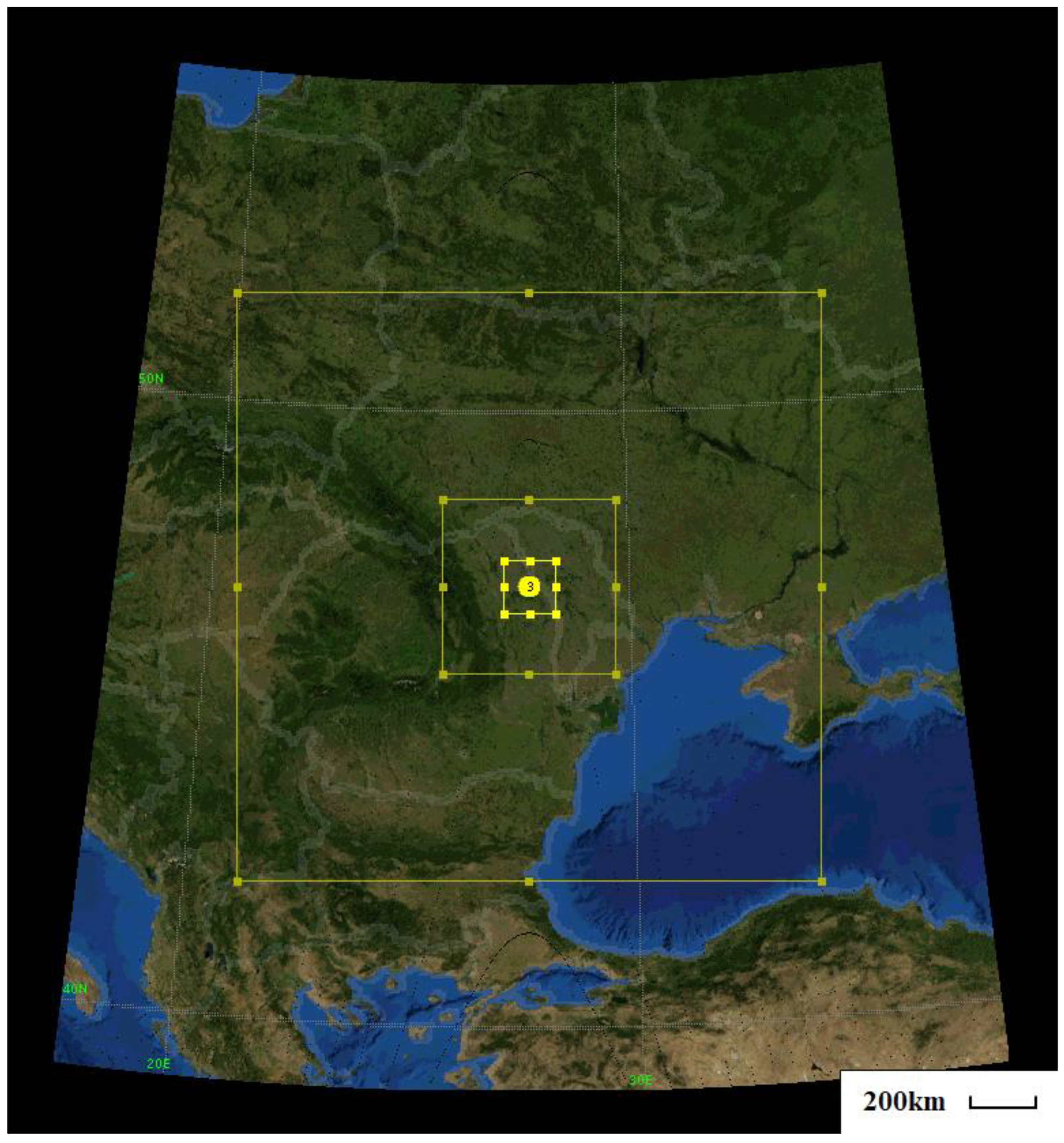
In this study, we used WRF version 3.9.1 with the Advanced Research WRF (ARW) dynamical solver [23]. Initial and boundary conditions were provided by IFS (Integrating Forecasting System) 6-hours analyses from ECMWF (European Centre for Medium-Range Weather Forecasts) with horizontal grid spacing of 0.125° × 0.125° in latitude and longitude. Three nested model domains were configured with varying horizontal grid spacing at the parent European level (; 120 × 120 grid points), and two nested domains roughly encompassing the Romania-Moldova region (; 106 × 106 grid points) and the Iași county, along with the Moldavian Ungheni district (; 94 × 94 grid points) (Figure 1 and Figure 2). It is assumed that 1 km × 1 grid spacing is of fine enough detail to resolve most mesoscale features in the complex study area [24]. In the simulations, 50 vertical levels were arranged between the surface and the 100 upper boundary.
Two events were studied, the first occurring from 16 May 2017 at 18:00 UTC to 17 May 2017 at 12:20 UTC and the second on the 4 April 2016 from 00:00 to 18:20 UTC. These two events were characterised by clear sky and a lack of precipitation; registered temperature, pressure and average wind speed show a relatively calm atmosphere. Atmospheric conditions are mostly fair for both events. Given that all the real data used to compare simulated WRF data are collected from instruments located in the city of Iași, data from the centre of the 3rd nest and the particularities of this nest will form the main objective of analysis in this study.
The geographical and seasonal particularities of the chosen area provide an interesting context and justification for this study. The area delineated by the 3rd nest is, under the Köppen–Geiger climate classification system [25], classified as Dfb (humid continental, without dry season, with warm summer) [26]. Multiple hills dot the area, with the highest point in the nest being at AGL, at Hîrtop Hill, and the lowest point being AGL, near the village of Gorban. Most of the rivers and rivulets (such as Bahlui and Jijia) flow south-eastwards into the larger Prut river, the natural border between Romania and the Republic of Moldova. The southern part of the nested area is heavily forested, while the northern part contains a large number of small bodies of water, such as the lakes Bulbucani, Hălcești, and even a fish farm destined for pisciculture and research [27]. In any case, the majority of the area is complex continental landmass, which can pose a challenge for the model; as opposed to simulations above flat, horizontal and homogeneous terrain, where the PBL height varies relatively slowly in space [28,29]. In terms of anthropogenic activity, the majority of the area is rural, with the largest by far urban area being the city of Iași, positioned at the centre of the nested area. The city has the second largest population in Romania [30], and a booming industrial and infrastructure sector [31]. According to the 2018 AirVisual World Air Quality Report, Iași is the most polluted city in Romania [32]. Topologically, the city stretches over at least seven hills, and is traversed by the river Bahlui. Overall, the anthropogenic influence of the central city and the geographic diversity of the area make for a suitable and interesting target for WRF simulations; especially in terms of the evolution of the PBL height in time.
In the present work, the sensitivity of some PBL schemes has been analysed. The PBL parametrizations available in WRF model and applied here consist of: YSU (YonSei University) scheme [33], MYJ (Mellor–Yamada–Janjic) scheme [34], ACM2 (Asymmetrical Convective Model version 2) scheme [35], BouLac (Bougeault–Lacarrère) scheme [36], TEMF (Total Energy–Mass Flux) scheme [37] and ShinHong scheme [38]. The first and most widely used PBL scheme is the YSU. It is a first-order, non-local scheme with an explicit entrainment layer and a parabolic K-profile in an unstable mixed layer, where PBLH in the YSU scheme is determined from the (bulk Richardson number) method but calculated starting from the surface. The MYJ scheme is a one-and-a-half order prognostic TKE scheme with local vertical mixing. The ACM2 scheme is a first-order, non-local closure scheme and features non-local upward mixing and local downward mixing. This scheme has an eddy-diffusion component in addition to the explicit non-local transport of ACM1 (Asymmetrical Convective Model version 1). PBLH is determined as the height where the Rib calculated above the level of neutral buoyancy exceeds a critical value (). For stable or neutral flows the scheme shuts off non-local transport and uses local closure. The BouLac scheme is a one-and-a-half order, local closure scheme and has a TKE prediction option designed for use with the BEP (Building Environment Parametrization) multi-layer, urban canopy model [39]. BouLac diagnoses PBLH as the height where the prognostic TKE reaches a sufficiently small value (in the current version of WRF is ). The TEMF scheme is a one-and-a-half order, non-local closure scheme and has a sub-gridscale total energy prognostic variable, in addition to mass-flux-type shallow convection. TEMF uses eddy diffusivity and mass flux concepts to determine vertical mixing. PBLH is calculated through a method with zero as a threshold value. Finally, the Shin-Hong PBL scheme is a scale-aware scheme. The subgrid scale transport profile is parameterized based on the 2013 conceptual derivation documented in Shin and Hong [38]. First, the nonlocal transport by strong updrafts and local transport by the remaining small-scale eddies are separately calculated. Second, the subgrid scale nonlocal transport is formulated by multiplying a grid-size dependency function with the total nonlocal transport profile fitted to the large eddy simulation output.
Other parametrizations used in this study are as follows: short and long-wave radiation parametrizations are New Goddard Shortwave and Longwave Schemes. No cumulus parametrization is implemented. The microphysics parametrization is represented by the Milbrandt–Yau Double Moment Scheme, and the land surface model used is the Unified Noah Land Surface Model. Chosen feedback is 1; this results in two-way nesting.
3. Instrumentation
A variety of measuring equipment is used in this study to contrast and compare the influences of different parametrizations to the WRF output; the first of them is a lidar. These systems are utilized in the fields of high-resolution mapping, geodesy, archaeology, geography, atmospheric physics and many more. Performing atmospheric altitude profiles of meteorological parameters in general demands specialized instrumentation and data processing. A standard and reliable method to directly obtain meteorological parameters throughout the free atmosphere for low to high altitudes is by launching specialized weather balloons equipped with in-situ sensors [40]. Radar, sodar, and microwave radiometer platforms have also been used to determine PBLH, or other boundary layer-related quantities, in other studies [41,42,43]. Lidar systems combine many of the advantages gained from using these instruments into one remote sensing platform, that is capable of returning atmospheric data profiles with a high temporal and spatial resolution [44,45,46].
The technical specifications of the main components of the lidar platform utilized in the study are as follows: the laser component is a Nd:YAG, producing pulses of laser at a frequency of , with a wavelength of , laser beam diameter of and a pulse energy of ; meanwhile, the optical component is a Newtonian LightBridge telescope with a primary mirror diameter of . The signal overlap altitude in most cases is approximately 200, much lower than most PBLH instances in general, and lower than all PBLH instances measured in this study. The lidar platform utilized in the study has a spatial resolution of and both technical details and results from previous measurement campaigns were reported in the scientific literature [47,48].
A common use for a lidar system, in the context of atmospheric physics, is the obtaining of PBLH data [49,50]; in this study, a method detailed in one of our previous studies is used [44]. This method consists of producing an arbitrary equation that highlights the PBL as a clear and sharp peak, which allows us to extract its height and plot its evolution in time [44]:
in which is the scintillation profile of the RCS (Range Corrected Signal) obtained by lidar, and is the backscatter coefficient profile obtained from RCS data via the Fernald-Klett inversion [51]. Our previous investigation shows that this equation can be used to retrieve the PBL height with greater confidence than other established methods, such as the gradient and the variance methods [44,49,50]. Regarding the potential influence of noise-related errors to the calculation of the scintillation profile, the overall signal uncertainty added by noise is:
where is raw lidar signal, is background lidar signal, and is the “noise scale factor”, which is equal to the standard deviation of the shot noise divided by the square root of average shot noise [52]. It is determined that the signal uncertainty, in the case of attenuated backscatter, has values of the order or lower [52], while a typical attenuated backscatter profile has values of the order or lower; thus, this uncertainty represents variations hundreds of times smaller than the actual values of the profile. Since the model subtracts the “dark” signal (generated by photocathode thermionic emission, which is collected before the measurements begin [53]) from the raw signal, we can assume that such uncertainty is even lower. Also, the fact that the photomultiplier component of the lidar platform utilized in this study was being operated in analogue mode removes the need to consider possible instances of “afterpulsing”, which only takes place when a photomultiplier component is operated in a “pulse detection mode” [53]. Finally, the fact that the photomultiplier component of the lidar platform used in this study is a PMT (photomultiplier tube) presents an advantage, since excess noise decreases with an increase in the average photo-multiplication gain in PMTs [52].
Another instrument that was used for data collecting and comparing purposes in this study is the sunphotometer, which is a type of photometer conceived in such a way that it points at the sun; the instrument used in the study is a Cimel Automatic Sun Tracking Photometer CE 318, which is a part of our AERONET Iasi_LOASL site [54,55]. While many of the higher applications of this instrument revolve around exploring aerosol properties in a given time and region [56,57], in this application the desired output of the instrument is the total precipitable water. Lidar and sunphotometer systems are sometimes used in conjunction [58]; a particular use for this coupling is to calculate the atmospheric aerosol backscatter profile [44,58]. The other instruments used to obtain GL data are located in the “Podul de Piatra” sector of Iași; data has been obtained from the ANM (Romanian National Meteorological Administration). The lidar, the photometer, and the GL instruments are located in three different sites, all of them situated, at most, 3 grid squares away from the center of the 3rd nest. All the measured values are compared accordingly to the simulated values in their own grid squares. There is just one GL monitoring station which contains all of the GL instruments, and there are no nearby natural or man-made structures that could present any obstruction to the instruments.
All operations of data manipulation and correlation were performed in Python 3.5, with Savitsky–Golay processing of real data profiles included in the plotting; this processing is a digital filter which can be applied to a set of points for the purpose of smoothing the data, through convolution [59,60]. The filter window chosen for this analysis is 17, and the order of the calculated fitting polynomial is 3; these numbers were chosen arbitrarily, in order to best fit the raw data from a graphical perspective. Finally, using the netCDF4 library, data from each WRF output file was extracted and compared to real data via plotting and evaluating statistical parameters.
4. Methods
In this section, the simulated data and instrument-related data are compared. The parameters of interest, extracted from WRF output, are the planetary boundary layer height (PBLH), atmospheric temperature at 2 AGL (T2M), average wind speed at 10 AGL (U10M), atmospheric pressure at 2 AGL (P2M), and the total precipitable water vapor (WV). This last value refers to the total atmospheric water vapor contained in a vertical column of unit cross-sectional area extending between any two specified levels, commonly expressed in terms of the height to which that water substance would stand if completely condensed and collected [61]. Following this definition, the total precipitable water vapor can be generally calculated with:
where is the density of water, gravitational acceleration, and the mixing ratio at a pressure level [61]. This definition is used since the mixing ratio profile is given as straight-forward output by the WRF simulation. Considering as the GL pressure, and the pressure at the maximum altitude at which WRF simulates the mixing ratio, the previous equation is re-written as:
Note that the use of this metric can imply the assumption that all the water vapor in the analyzed region is concentrated in the PBL; it is certain that if this were the case, PBLH parametrizations would play a much higher role in influencing simulated WV. However, while this assumption is not made here, it is fair to assume that any small change in the water vapor content of the atmosphere would influence the PBL in some manner, and the opposite can also be assumed. Indeed, it can be seen in the following results segment that changes in PBLH parametrizations slightly influence the simulated WV. The statistical measures used to verify and contrast the WRF simulations are the mean absolute error (MAE), mean bias error (MBE), root mean square error (RMSE) and coefficient of determination ().
5. Results
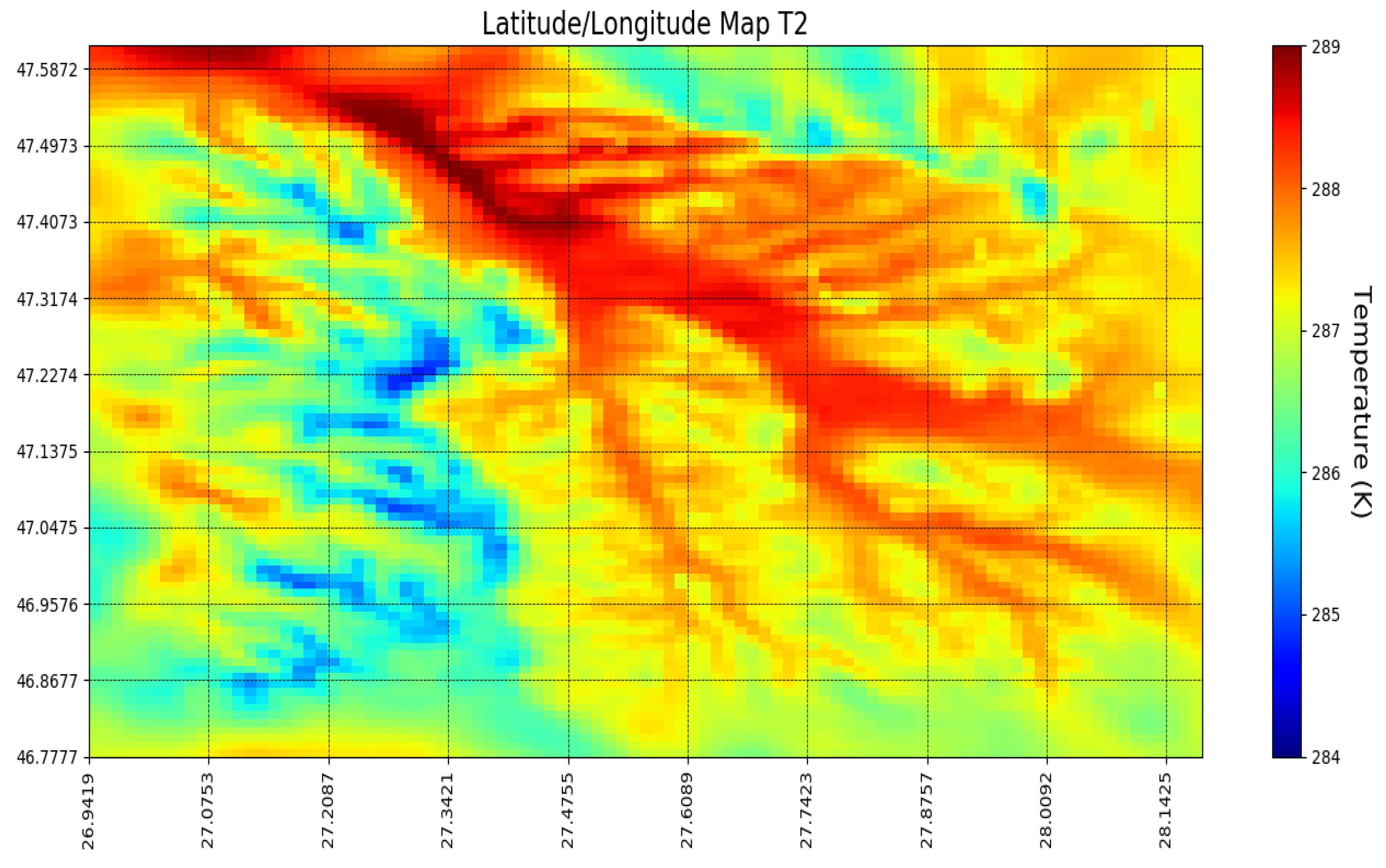
PBLH and T2M maps in the inner domain were obtained from the WRF simulations as examples. The outputs computed with YSU parametrization at 08:00 UTC in both episodes are shown in Figure 3, Figure 4, Figure 5 and Figure 6. The temperature at 2 meters from the surface is lower and less variable on 17 May 2017 (Figure 5) than on 4 April 2016 (Figure 6) when the maximum values are reached along and across the Prut river basin, where the altitude is lowest. As a consequence, the PBLH maps tend to show higher values in regions where their respective T2M maps show higher temperature; for the 2017 scenario, that is roughly the region of the Prut river basin, and for the 2016 scenario, the hills south of Iași.
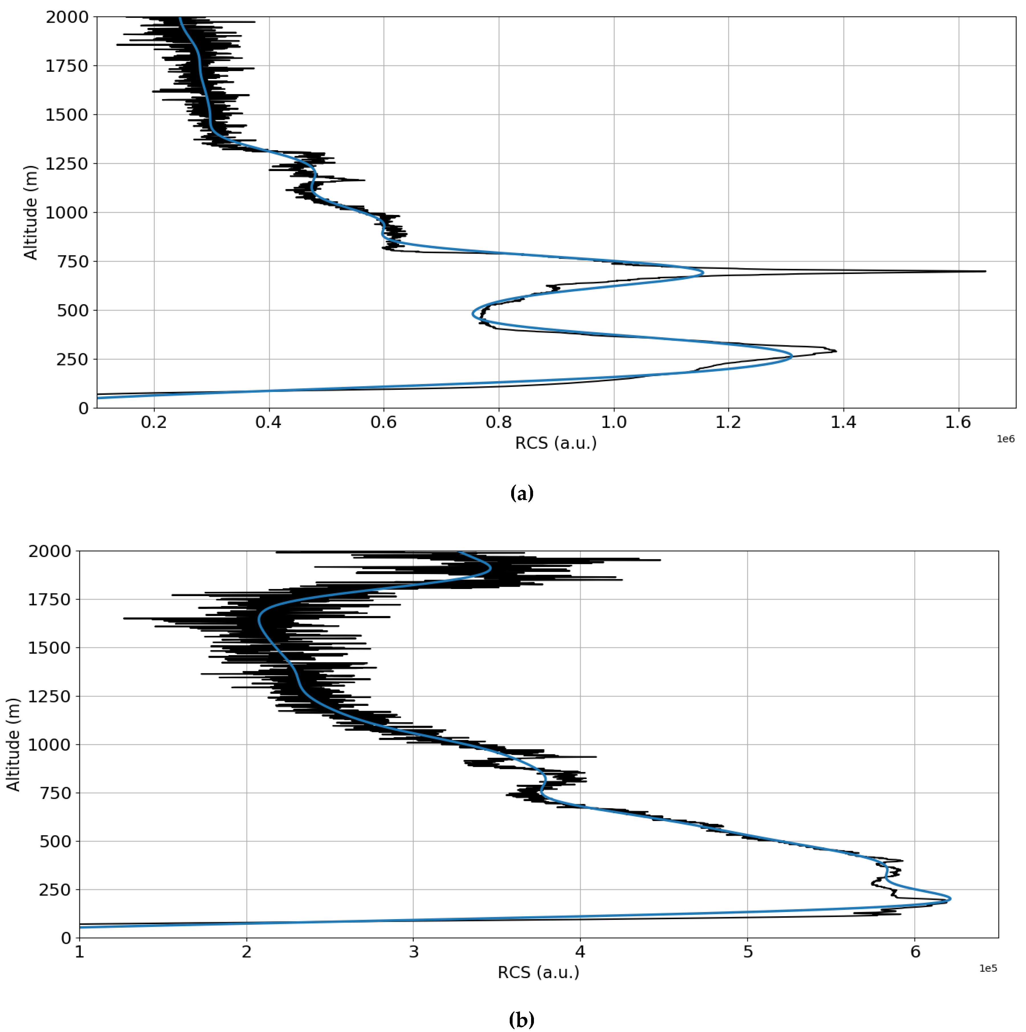
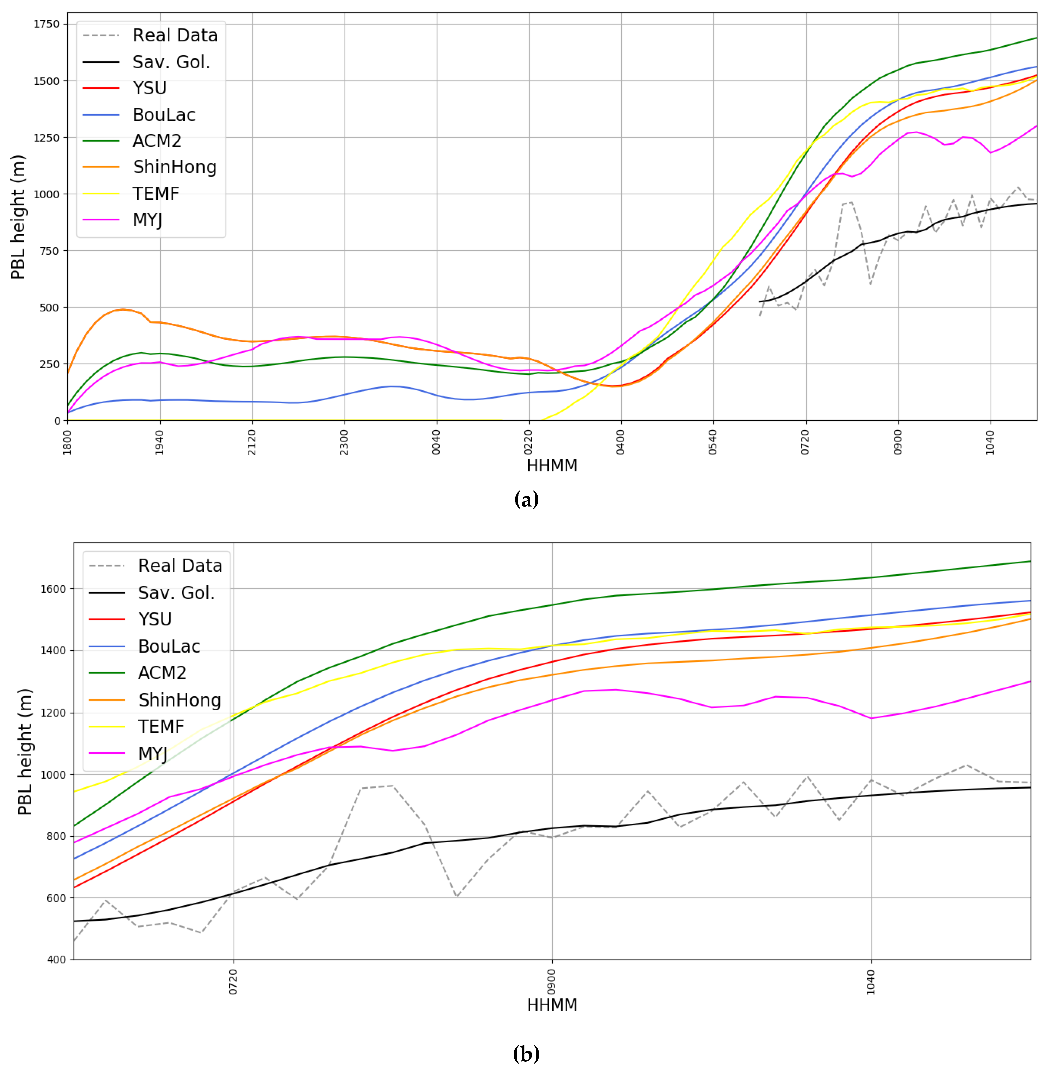
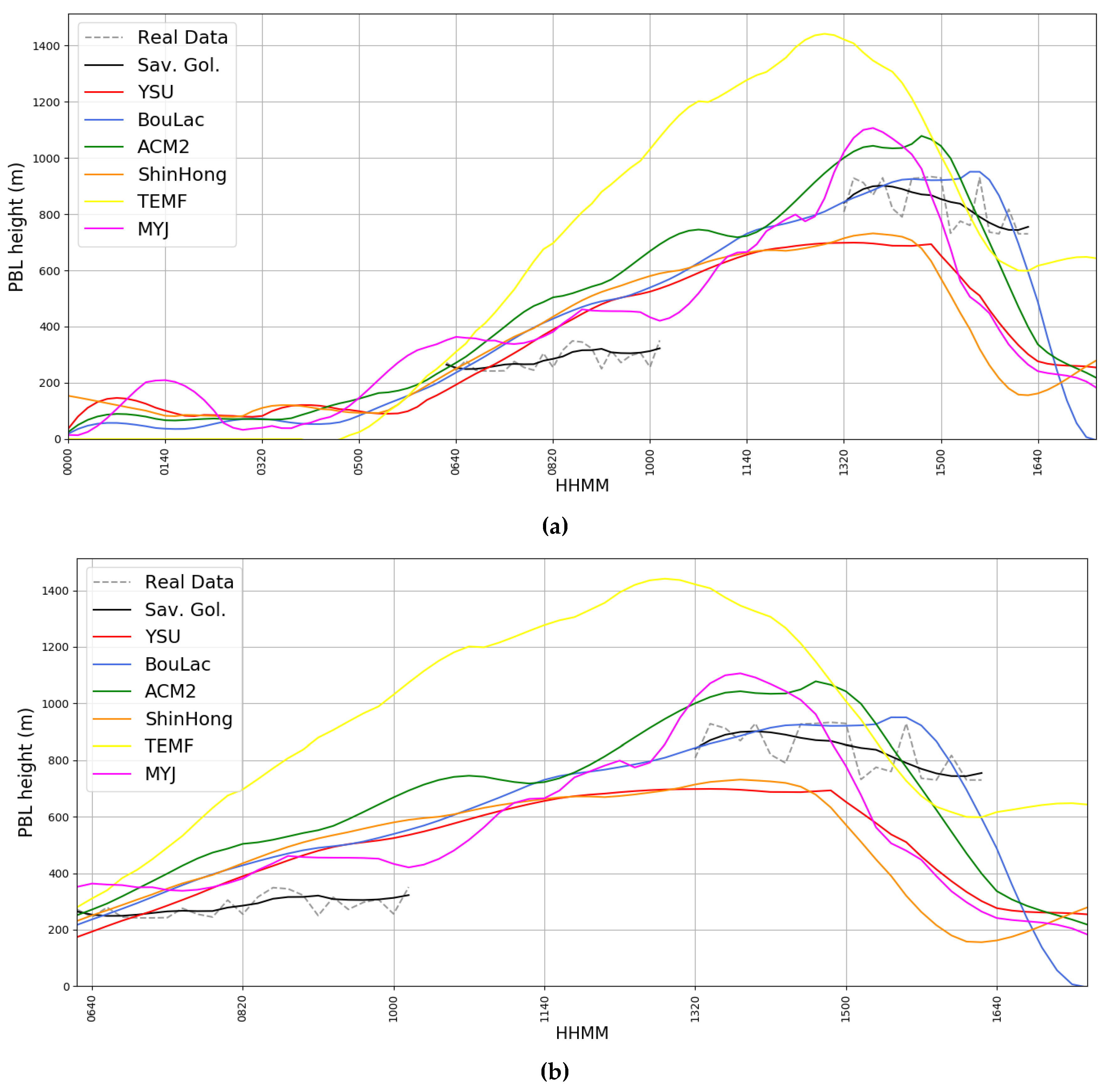
In the following, the WRF output and the obtained data comparison are introduced by means of both graphical and table data. First, two examples of RCS data for each scenario are presented, in order to exemplify the typical signal obtained by the platform used in this study, and to determine that the PBLH is not lower than the complete signal overlap altitude (Figure 7). WRF results on 17 May 2017 show that the different parametrizations compute a nocturnal PBLH lower than 500 and a diurnal that is always higher than the observed one (Figure 8). During the 4 April 2016 episode simulated PBLH values are lower than 200 and their maxima occur between 13:00 and 15:00 UTC. The comparison with observation shows that simulated PBLH values are higher than observed ones in the morning, and in agreement with observations in the afternoon (Figure 9). The PBL parametrizations have similar performances with the exception of TEMF, during 4 April 2016 episode, which seems to not catch the general PBLH trend. MAE and RMSE values between each parametrization and lidar data, and each parametrization with each other (Table 1 and Table 2) indicate that MYJ is the best performing parametrization in the episode of 17 May 2017; the same is true for YSU and BouLac parametrizations in the episode of 4 April 2016, while values show a generally high correlation, with ACM2 performing best for the 2017 episode, and ShinHong performing best for the 2016 episode.
Simulated and observed temperature values are well correlated, and mean difference is under one degree Celsius in most cases (Figure 10 and Figure 11) (Table 1 and Table 2). The different simulations have similar behaviours with the exception of TEMF scheme that, in the 4 April episode, is unable to describe the temperature time trend.
The two events were characterised by low wind speed. During the first episode (Figure 12) the average wind speed was lower than 2 at night and reached 3 in the morning. All six PBL parametrizations correctly compute the low wind regime during the night and the increasing wind speed values from 4:00 UTC. The second episode (Figure 13) is characterised by a calm atmosphere with wind speeds less than 1.5. Also, in this case, all six simulations were able to identify the low wind regime. Therefore, MAE, MBE, and RMSE values for all simulations are generally lower than 1 and a categorically-best parametrization cannot be found. Average wind speed is quite poorly correlated; however, such variation is to be partly expected, considering the low values of this average wind speed (Figure 12 and Figure 13) (Table 1 and Table 2).
Pressure data is inconclusive; one case shows low correlation, another shows high correlation, yet both cases present relatively low mean difference compared to value evolution in time (Figure 14 and Figure 15) (Table 1 and Table 2). However, simulated pressure values from different parametrizations are very similar to one another. They differ from simulated ones regarding the trend, but the values are comparable. Statistical values of MAE, MBE and RMSE show a general common performance for all simulations.
The total precipitable water is consistently underestimated by all the WRF simulations by about 0.5 cm but the variation in time seems to be, however, appropriately predicted (Figure 16 and Figure 17) (Table 1 and Table 2). values show a decent correlation at best, because of a constantly significant mean difference and no interception between simulated and measured data. The above-mentioned Unified Noah Land Surface Model used in this simulation, judging from the original paper that introduces it [62], seems to show an increased sensitivity to variations of soil moisture, which might partly account for the difference in the total measured and simulated water vapor. However, such an error due to excessive sensitivity to soil moisture would also mean that the evolution of the total water vapor would be different from the simulated one: the fact that WRF manages to simulate quite accurately the evolution but not the quantity of total water vapor gives us reason to believe that the difference in simulated and observed values is due to unpredicted phenomena of water vapor transport and advection in the atmosphere. Another likely possibility is that these errors are caused by a dry bias in the initial or boundary conditions provided to WRF through the ECMWF data; a validation study has shown that instances of such a bias can appear for data over several complex terrains, which would certainly explain the differences between simulated and observed WV values [63].
Strictly in terms of the MAE, for the 2017 data set, the MYJ parametrization obtained the best results with the PBLH and T2M evolution whereas much of the simulated data using the TEMF parametrization is highly inaccurate when compared to the PBLH and T2M sets of data obtained in 2016 (Figure 9 and Figure 11, Table 2). In the case of P2M and WV, TEMF shows the smallest error, while the ShinHong parametrization is superior in the case of U10M (Table 1 and Table 2). For the 2016 data set, T2M and U10M data are best modelled with MYJ, while TEMF and ShinHong are best in terms of the P2M and WV evolution respectively, and the BouLac parametrization obtains the best results regarding the PBLH evolution (Table 1 and Table 2). YSU also yields satisfactory simulations in most cases, while the ACM2 parametrization seems to obtain consistently poor results.
Note that there are two instances when WRF simulations present consistent errors when compared to observed data: in both episodes, PBLH evolution is overestimated in the morning, and in both episodes, WV is underestimated (despite the fact that the evolution seems correctly predicted). There is also the problem with apparent simulation anomalies given when the model employs the TEMF parametrization. Numerous similarities can be identified between this parametrization and all the others, such as the order and non-locality; however, what this scheme seems to have as a substantial difference is the calculation of PBLH through a method with zero as a threshold value. It is possible that this method is problematic for the simulations at hand and is unsuitable in the analyzed cases.
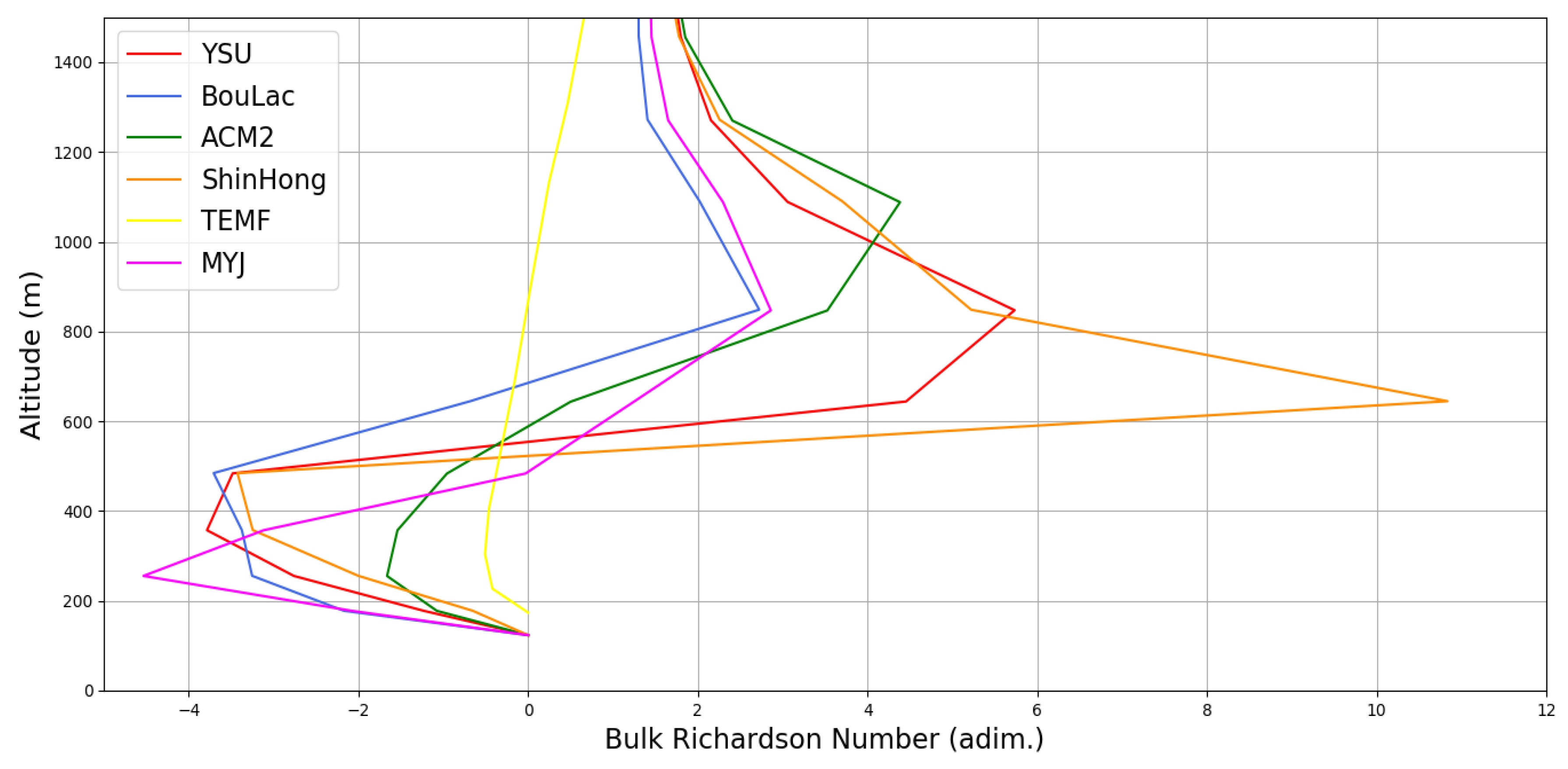
In order to test this possibility, two series of representative profiles have been made using data simulated for the 2016 episode to test if the behaviour of the profile made with the TEMF parametrization is also anomalous (Figure 18 and Figure 19). These two series correspond to the two lidar measurement intervals in the 2016 episode, and the data has been picked so as to roughly match the middle of both of the lidar measurement intervals. The profiles are made as per the typical bulk Richardson number profile, using wind speed and potential temperature WRF output data [64]; they have not been smoothed with a Savitsky–Golay filter in order to show with a greater deal of precision the altitudes at which these profiles reach . As expected, the profiles do show that TEMF produces a profile that is vastly different from the others; one would logically expect that a lower would produce a lower estimation of the PBLH, in opposition with the simulated PBLH values at hand. However, what is instead observed is that the TEMF-produced profile remains negative at higher altitudes, approaching positive values at a much slower rate (Figure 18 and Figure 19). Thus, the critical TEMF is reached at higher altitudes than in the case of other parametrizations, resulting in an innacurate or anomalous simulated PBLH. Another interesting conclusion that can be extracted from the figures is that the values simulated with all parametrizations become quite similar to one another at higher altitudes, except for TEMF (Figure 18 and Figure 19).
6. Conclusion
Different PBL parametrization schemes in WRF framework were applied over a complex area crossed by rivers and including urban and rural zones. The simulated data were compared with observations from traditional surface instrumentation and a lidar system. A future study, facilitated by a suitable computational platform might include more sets of simulated data across multiple seasons, and a greater degree of experimentation with parametrizations pertaining to multiple aspects of the atmosphere.
The application of WRF in the selected timeframes and the selected region seems to yield, with most PBLH parametrizations, a boundary layer that is deeper in some cases from the obtained observed data. PBLH evolution is, on average, quite well modelled with the MYJ and also with YSU performing decently, with the exception of slight overestimations at the early hours of the episodes. Temperature seems to be the selected value that is consistently well-approximated. Wind speed regime is well represented in the case of low intensities, and this is done in both simulation episodes. Pressure values are equally well identified by all parametrizations, but the trend is not always correctly identified.
Given the various seasonal peculiarities, and the challenging geographic and anthropogenic complexity of the examined region, it can be said that the model performed well in the case of most chosen parameters; in the case of ground-level temperature, for example, studies show that differences of two to three degrees Celsius between WRF simulated and real data are not uncommon; nor are differences of more than 0.3 in the case of PBL height [3,4,5,6]. These studies also seem to point out that such differences can increase in warm seasons. The comparisons show that multiple improvements can be made to WRF parametrizations for the specific region of Iași in the warm season, especially regarding the transport of precipitable water vapour in the atmosphere, and the early-morning evolution of the PBL. Additionally, simulations using the TEMF parametrization may present certain anomalous values, which most likely arise from the PBLH calculation that uses zero as the threshold in its method.
Author Contributions
Conceptualization, R.L.-A., F.S. and C.M.M.; Data curation, R.L.-A., F.S., R.I. and C.M.M.; methodology, R.L.-A., F.S. and C.M.M.; software, R.L.-A. and F.S.; Supervision, R.L.-A., F.S. and C.M.M.; validation, R.L.-A. and F.S.; Visualization, F.S. and C.M.M.; formal analysis, R.L.-A., F.S., R.I., C.V. and C.M.M.; resources, R.L.-A., F.S., C.V. and C.M.M.; writing—original draft preparation, R.L.-A., F.S. and C.M.M.; writing—review and editing, R.L.-A., F.S., R.I., C.V. and C.M.M..; project administration, R.L.-A., F.S. and C.M.M.; funding acquisition, C.M.M.; Investigation, R.L.-A., F.S., R.I., C.V. and C.M.M.
Funding
This work was supported by a research grant of the TUIASI, project number GnaC2018_65/2019.
Conflicts of Interest
The authors declare no conflict of interest.
References
- Rao, K.S. Uncertainty analysis in atmospheric dispersion modeling. Pure Appl. Geophys. 2005, 162, 1893–1917. [Google Scholar] [CrossRef]
- Selvam, A.M. Nonlinear dynamics and chaos: Applications in atmospheric sciences. J. Adv. Math. Appl. 2012, 1, 181–205. [Google Scholar] [CrossRef]
- Timofte, A.; Belegante, L.; Cazacu, M.M.; Albina, B.; Talianu, C.; Gurlui, S. Study of planetary boundary layer height from LIDAR measurements and ALARO model. J. Optoelectron. Adv. Mater. 2015, 17, 911–917. [Google Scholar]
- Banks, R.F.; Tiana-Alsina, J.; Baldasano, J.M.; Rocadenbosch, F.; Papayannis, A.; Solomos, S.; Tzanis, C.G. Sensitivity of boundary-layer variables to PBL schemes in the WRF model based on surface meteorological observations, lidar, and radiosondes during the HygrA-CD campaign. Atmos. Res. 2016, 176, 185–201. [Google Scholar] [CrossRef]
- Belegante, L.; Nicolae, D.; Nemuc, A.; Talianu, C.; Derognat, C. Retrieval of the boundary layer height from active and passive remote sensors. Comparison with a NWP model. Acta Geophys. 2014, 62, 276–289. [Google Scholar] [CrossRef]
- García-Díez, M.; Fernández, J.; Fita, L.; Yagüe, C. Seasonal dependence of WRF model biases and sensitivity to PBL schemes over Europe. Q. J. R. Meteorol. Soc. 2013, 139, 501–514. [Google Scholar] [CrossRef]
- Banks, R.F.; Tiana-Alsina, J.; Rocadenbosch, F.; Baldasano, J.M. Performance evaluation of the boundary-layer height from lidar and the Weather Research and Forecasting model at an urban coastal site in the north-east Iberian Peninsula. Bound. Layer Meteorol. 2015, 157, 265–292. [Google Scholar] [CrossRef]
- Boadh, R.; Satyanarayana, A.N.V.R.; Krishna, T.V.B.P.S.; Madala, S. Sensitivity of PBL schemes of the WRF-ARW model in simulating the boundary layer flow parameters for their application to air pollution dispersion modelling over a tropical station. Atmosfera 2016, 29, 61–81. [Google Scholar] [CrossRef]
- Milovac, J.; Warrach-Sagi, K.; Behrendt, A.; Späth, F.; Ingwersen, J.; Wulfmeyer, V. Inversigation of PBL schemes combining the WRF model simulations with scanning water vapor differential abseorption lidar measurements. J. Geophys. Res. Atmos. 2015, 121, 624–649. [Google Scholar] [CrossRef]
- Sathyanadh, A.; Prabha, T.V.; Balaji, B.; Resmi, E.A.; Karipot, A. Evaluation of WRF PBL parametrization schemes against direct observations during a dry event over the Ganges valley. Atmos. Res. 2017, 193, 125–141. [Google Scholar] [CrossRef]
- Pérez, C.; Jiménez, P.; Jorba, O.; Sicard, M.; Baldasano, J.M. Influence of the PBL scheme on high-resolution photochemical simulations in an urban coastal area over the Western Mediterranean. Atmos. Environ. 2006, 40, 5274–5297. [Google Scholar] [CrossRef]
- Bossioli, E.; Tombrou, M.; Dandou, A.; Athanasopoulou, E.; Varotsos, K.V. The role of planetary boundary-layer parameterizations in the air quality of an urban area with complex topography. Bound. Layer Meteorol. 2009, 131, 53–72. [Google Scholar] [CrossRef]
- Dudhia, J. A nonhydrostatic version of the Penn State–NCAR mesoscale model: Validation tests and simulation of an Atlantic cyclone and cold front. Mon. Weather Rev. 1993, 121, 1493–1513. [Google Scholar] [CrossRef]
- Lupașcu, A.; Iriza, A.; Dumitrache, R.C. Using a high resolution topographic data set and analysis of the impact on the forecast of meteorological parameters. Rom. Rep. Phys. 2015, 67, 653–664. [Google Scholar]
- Iriza, A.; Dumitrache, R.C.; Ştefan, S. Numerical modelling of the Bucharest urban heat island with the WRF-urban system. Rom. J. Phys. 2017, 62, 1–14. [Google Scholar]
- Isvoranu, D.; Badescu, V. Comparison Between Measurements and WRF Numerical Simulation of Global Solar Irradiation in Romania. Ann. West. Univ. Timis. Phys. 2013, 57, 24–33. [Google Scholar] [CrossRef] [Green Version]
- Dimitrova, R.; Danchovski, V.; Egova, E.; Vladimirov, E.; Sharma, A.; Gueorguiev, O.; Ivanov, D. Modeling the Impact of Urbanization on Local Meteorological Conditions in Sofia. Atmosphere 2019, 10, 366. [Google Scholar] [CrossRef]
- Run, R.; Case, R.D.T. User’s Guide for the NMM Core of the Weather Research and Forecast (WRF) Modeling System Version 3. Available online: https://dtcenter.org/wrf-nmm/users/docs/user_guide/V3/contents_nmm.pdf (accessed on 15 June 2019).
- Morille, Y.; Haeffelin, M.; Drobinski, P.; Pelon, J. STRAT: An automated algorithm to retrieve the vertical structure of the atmosphere from single-channel lidar data. J. Atmos. Ocean. Technol. 2007, 24, 761–775. [Google Scholar] [CrossRef]
- Hennemuth, B.; Lammert, A. Determination of the atmospheric boundary layer height from radiosonde and lidar backscatter. Bound. Layer Meteorol. 2006, 120, 181–200. [Google Scholar] [CrossRef]
- Weather Research and Forecasting Model. Available online: https://www.mmm.ucar.edu/weather-research-and-forecasting-model (accessed on 10 May 2019).
- Powers, J.G.; Klemp, J.B.; Skamarock, W.C.; Davis, C.A.; Dudhia, J.; Gill, D.O.; Grell, G.A. The weather research and forecasting model: Overview, system efforts, and future directions. Bull. Am. Meteorol. Soc. 2017, 98, 1717–1737. [Google Scholar] [CrossRef]
- Skamarock, W.C.; Klemp, J.B.; Dudhia, J.; Gill, D.O.; Barker, D.M.; Wang, W.; Powers, J.G. A Description of the Advanced Research WRF Version 2; No. NCAR/TN-468+ STR; National Center for Atmospheric Research: Boulder, Co, USA; Mesoscale and Microscale Meteorology Div.: Boulder, CO, USA, 2015. [Google Scholar]
- Jiménez, P.A.; Dudhia, J.; González-Rouco, J.F.; Montávez, J.P.; García-Bustamante, E.; Navarro, J.; Muñoz-Roldán, A. An evaluation of WRF's ability to reproduce the surface wind over complex terrain based on typical circulation patterns. J. Geophys. Res. Atmos. 2013, 118, 7651–7669. [Google Scholar] [CrossRef] [Green Version]
- Geiger, R. Klassifikation Der Klimate Nach W. Köppen (Classification of Climates after W. Köppen); Landolt-Börnstein—Zahlenwerte und Funktionen aus Physik, Chemie, Astronomie, Geophysik und Technik, alte Serie; Springer: Berlin, Germany, 1954; Volume 3, pp. 603–607. [Google Scholar]
- Peel, M.C.; Finlayson, B.L.; McMahon, T.A. Updated world map of the Köppen−Geiger climate classification. Hydrol. Earth Syst. Sci. 2007, 11, 1633–1644. [Google Scholar] [CrossRef]
- Pisciculture Tiganasi. Available online: https://www.producator-agricol.ro/piscicultura/tiganasi (accessed on 1 July 2019).
- Stull, R.B. An Introduction to Boundary Layer Meteorology; Kluwer Academic Publishers: Dordrecht, The Netherlands; Boston, MA, USA; London, UK, 1988; p. 666. [Google Scholar]
- Foken, T. Micrometeorolgy; Springer-Verlag: Berlin, Germany, 2016. [Google Scholar] [CrossRef]
- World Population Review. Available online: http://worldpopulationreview.com/countries/romania-population/cities/ (accessed on 1 July 2019).
- Aspen Economic Opportunities & Financing the Economy Program 2018. Available online: http://aspeninstitute.ro/white-paper-aspen-economic-opportunities-financing-the-economy-program-2018/ (accessed on 1 July 2019).
- AirVisual Database. Available online: https://www.airvisual.com/world-most-polluted-cities (accessed on 15 May 2019).
- Hong, S.Y.; Lim, J.O.J. The WRF single-moment 6-class microphysics scheme. Asia-Pac. J. Atmos. Sci. 2006, 42, 129–151. [Google Scholar]
- Janić, Z.I. Nonsingular implementation of the Mellor-Yamada level 2.5 scheme in the NCEP Meso model. Natl. Ocean. Atmos. Adm. 2001, 437, 1–61. [Google Scholar]
- Pleim, J.E. A combined local and nonlocal closure model for the atmospheric boundary layer. Part I: Model description and testing. J. Appl. Meteorol. Climatol. 2007, 46, 1383–1395. [Google Scholar] [CrossRef]
- Bougeault, P.; Lacarrere, P. Parameterization of orography-induced turbulence in a mesobeta--scale model. Mon. Weather Rev. 1989, 117, 1872–1890. [Google Scholar] [CrossRef]
- Angevine, W.M.; Jiang, H.; Mauritsen, T. Performance of an eddy diffusivity–mass flux scheme for shallow cumulus boundary layers. Mon. Weather Rev. 2010, 138, 2895–2912. [Google Scholar] [CrossRef]
- Shin, H.H.; Hong, S.Y. Analysis of resolved and parameterized vertical transports in convective boundary layers at gray-zone resolutions. J. Atmos. Sci. 2013, 70, 3248–3261. [Google Scholar] [CrossRef]
- Martilli, A.; Clappier, A.; Rotach, M.W. An urban surface exchange parameterisation for mesoscale models. Bound.-Layer Meteorol. 2002, 104, 261–304. [Google Scholar] [CrossRef]
- Durre, I.; Vose, R.S.; Wuertz, D.B. Robust automated quality assurance of radiosonde temperatures. J. Appl. Meteorol. Climatol. 2008, 47, 2081–2095. [Google Scholar] [CrossRef]
- Kropfli, R.A. A review of microwave radar observations in the dry convective planetary boundary layer. Bound.-Layer Meteorol. 1983, 26, 51–67. [Google Scholar] [CrossRef]
- Beyrich, F.; Görsdorf, U. Composing the diurnal cycle of mixing height from simultaneous sodar and wind profiler measurements. Bound.-Layer Meteorol. 1995, 76, 387–394. [Google Scholar] [CrossRef]
- Cimini, D.; De Angelis, F.; Dupont, J.C.; Pal, S.; Haeffelin, M. Mixing layer height retrievals by multichannel microwave radiometer observations. Atmos. Meas. 2013, 6, 2941–2951. [Google Scholar] [CrossRef] [Green Version]
- Rosu, I.A.; Cazacu, M.M.; Prelipceanu, O.S.; Agop, M. A Turbulence-Oriented Approach to Retrieve Various Atmospheric Parameters Using Advanced Lidar Data Processing Techniques. Atmosphere 2019, 10, 38. [Google Scholar] [CrossRef]
- Lolli, S.; Madonna, F.; Rosoldi, M.; Campbell, J.R.; Welton, E.J.; Lewis, J.R.; Pappalardo, G.; Gu, Y. Impact of varying lidar measurement and data processing techniques in evaluating cirrus cloud and aerosol direct radiative effects. Atmos. Meas. Tech. 2018, 11, 1639–1651. [Google Scholar] [CrossRef] [Green Version]
- Reichardt, J.; Wandinger, U.; Klein, V.; Mattis, I.; Hilber, B.; Begbie, R. RAMSES: German Meteorological Service autonomous Raman lidar for water vapor, temperature, aerosol, and cloud measurements. Appl. Opt. 2012, 51, 8111–8131. [Google Scholar] [CrossRef] [PubMed]
- Belegante, L.; Cazacu, M.M.; Timofte, A.; Toanca, F.; Vasilescu, J.; Rusu, M.I.; Ajtai, N.; Stefanie, H.I.; Vetres, I.; Ozunu, A.; et al. Case study of the first volcanic ash exercise in Romania using remote sensing techniques. Environ. Eng. Manag. J. 2015, 14, 2503–2504. [Google Scholar]
- Papayannis, A.; Nicolae, D.; Kokkalis, P.; Binietoglou, I.; Talianu, C.; Belegante, L.; Tsaknakis, G.; Cazacu, M.M.; Vetres, I.; Ilic, L. Optical, size and mass properties of mixed type aerosols in Greece and Romania as observed by synergy of lidar and sunphotometers in combination with model simulations: A case study. Sci. Total Environ. 2014, 500, 277–294. [Google Scholar] [CrossRef] [PubMed]
- Flamant, C.; Pelon, J.; Flamant, P.H.; Durand, P. Lidar determination of the entrainment zone thickness at the top of the unstable marine atmospheric boundary layer. Bound. Layer Meteorol. 1997, 83, 247–284. [Google Scholar] [CrossRef]
- Haeffelin, M.; Angelini, F.; Morille, Y.; Martucci, G.; Frey, S.; Gobbi, G.P.; Lolli, S.; O’Dowd, C.D.; Sauvage, L.; Xueref-Rémy, I.; et al. Evaluation of mixing-height retrievals from automatic profiling lidars and ceilometers in view of future integrated networks in Europe. Bound. Layer Meteorol. 2012, 143, 49–75. [Google Scholar] [CrossRef]
- Klett, J.D. Stable analytical inversion solution for processing lidar returns. Appl. Opt. 1981, 20, 211–220. [Google Scholar] [CrossRef] [PubMed] [Green Version]
- Liu, Z.; Hunt, W.; Vaughan, M.; Hostetler, C.; McGill, M.; Powell, K.; Winker, D.M.; Hu, Y. Estimating random errors due to shot noise in backscatter lidar observations. Appl. Opt. 2006, 45, 4437–4447. [Google Scholar] [CrossRef] [PubMed]
- Hamamatsu, Photomultiplier Tubes, and Photomultipliers Tubes Photonics “Basics and Applications”; Hamamatsu Photonics KK: Iwata City, Japan, 2007.
- Unga, F.; Cazacu, M.M.; Timofte, A.; Bostan, D.; Mortier, A.; Dimitriu, D.G.; Gurlui, S.; Goloub, P. Study of tropospheric aerosol types over Iasi, Romania, during summer of 2012. Environ. Eng. Manag. J. 2013, 12, 297–303. [Google Scholar]
- Cazacu, M.M.; Timofte, A.; Unga, F.; Albina, B.; Gurlui, S. AERONET data investigation of the aerosol mixtures over Iasi area, One-year time scale overview. J. Quant. Spectrosc. Radiat. Transf. 2015, 15357–15364. [Google Scholar] [CrossRef]
- Ajtai, N.; Stefanie, H.; Arghius, V.; Meltzer, M.; Costin, D. Characterization of aerosol optical and microphysical properties over North-Western Romania in correlation with predominant atmospheric circulation patterns, International Multidisciplinary Scientific Geo Conference. Surv. Geol. Min. Ecol. Manag. 2017, 17, 375–382. [Google Scholar]
- Ajtai, N.; Stefanie, H.; Ozunu, A. Description of aerosol properties over Cluj-Napoca derived from AERONET sun photometric data. Environ. Eng. Manag. J. 2013, 12, 227–232. [Google Scholar] [CrossRef]
- Binietoglou, I.; Basart, S.; Alados-Arboledas, L.; Amiridis, V.; Argyrouli, A.; Baars, H.; Baldasano, J.M.; Balis, D.; Belegante, L.; Bravo-Aranda, J.A.; et al. A methodology for investigating dust model performance using synergistic EARLINET/AERONET dust concentration retrievals. Atmos. Meas. Tech. 2015, 8, 3577–3600. [Google Scholar] [CrossRef] [Green Version]
- Steinier, J.; Termonia, Y.; Deltour, J. Smoothing and differentiation of data by simplified least square procedure. Anal. Chem. 1972, 44, 1906–1909. [Google Scholar] [CrossRef]
- Savitzky, A.; Golay, M.J. Smoothing and differentiation of data by simplified least squares procedures. Anal. Chem. 1964, 36, 1627–1639. [Google Scholar] [CrossRef]
- Glossary of Meteorology. Available online: http://glossary.ametsoc.org/wiki/Precipitable_water (accessed on 1 June 2019).
- Tewari, M.; Chen, F.; Wang, W.; Dudhia, J.; LeMone, M.A.; Mitchell, K.; Cuenca, R.H. Implementation and verification of the unified NOAH land surface model in the WRF model. In 20th Conference on Weather Analysis and Forecasting/16th Conference on Numerical Weather Prediction; American Meteorological Society: Seattle, WA, USA, 2004; Volume 1115. [Google Scholar]
- Bock, O.; Keil, C.; Richard, E.; Flamant, C.; Bouin, M.N. Validation of precipitable water from ECMWF model analyses with GPS and radiosonde data during the MAP SOP. Q. J. R. Meteorol. Soc. A J. Atmos. Sci. Appl. Meteorol. Phys. Oceanogr. 2005, 131, 3013–3036. [Google Scholar] [CrossRef]
- Zhang, Y.; Gao, Z.; Li, D.; Li, Y.; Zhang, N.; Zhao, X.; Chen, J. On the computation of planetary boundary-layer height using the bulk Richardson number method. Geosci. Model. Dev. 2014, 7, 2599–2611. [Google Scholar] [CrossRef] [Green Version]
Figure 1.
Three nested model domains used in this study (yellow lines). 1st nest: contains the entirety of Romania and Republic of Moldova, along with the area around it and sections of neighboring countries. 2nd nest: contains larger Moldova and Bucovina region of Romania, and the majority of the Republic of Moldova. 3rd nest: contains area around the city of Iași. Number 3 (in yellow circle) represents the city of Iași.

Figure 2.
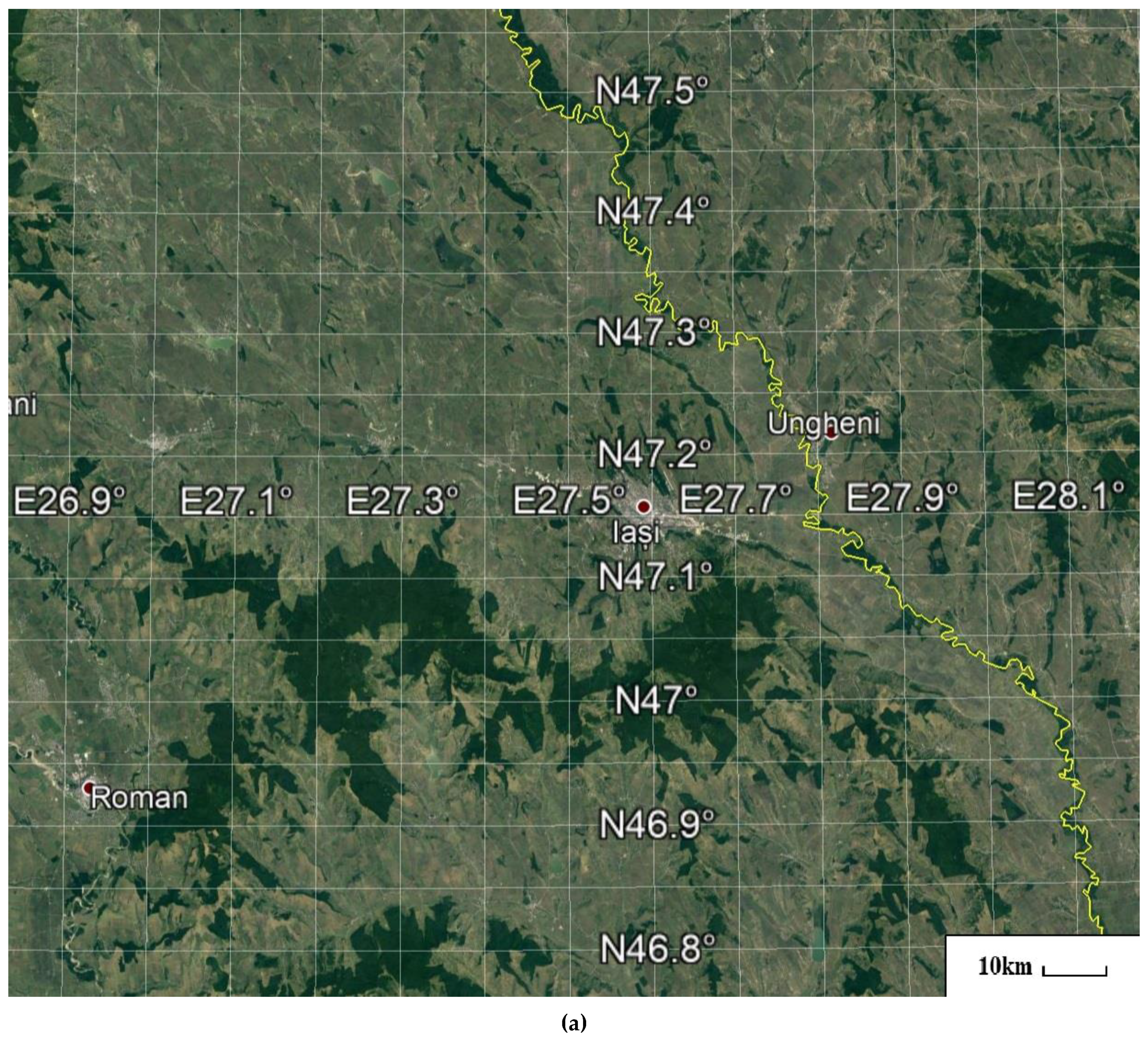
(a) Satellite map of the 3rd nest with latitude/longitude grid; border between Romania (right) and Moldova (left) delineated by the Prut river (yellow line); Google Earth. (b) Relief map of the 3rd nest with latitude/longitude grid; border between Romania (right) and Moldova (left) delineated by the Prut river (yellow line); altitude colormap: ~5 m above ground-level (AGL) dark green, ≤300 m AGL bright yellow; Google Earth.
Figure 2.
(a) Satellite map of the 3rd nest with latitude/longitude grid; border between Romania (right) and Moldova (left) delineated by the Prut river (yellow line); Google Earth. (b) Relief map of the 3rd nest with latitude/longitude grid; border between Romania (right) and Moldova (left) delineated by the Prut river (yellow line); altitude colormap: ~5 m above ground-level (AGL) dark green, ≤300 m AGL bright yellow; Google Earth.


Figure 3.
Example of a Weather Research and Forecasting (WRF) output map (PBLH); 3rd nest, in center of nest: Iași; 17/05/2017, 08:00 UTC; YSU parametrization.
Figure 3.
Example of a Weather Research and Forecasting (WRF) output map (PBLH); 3rd nest, in center of nest: Iași; 17/05/2017, 08:00 UTC; YSU parametrization.

Figure 4.
Example of a WRF output map (PBLH); 3rd nest, in center of nest: Iași; 04/04/2016, 08:00 UTC; YSU parametrization.
Figure 4.
Example of a WRF output map (PBLH); 3rd nest, in center of nest: Iași; 04/04/2016, 08:00 UTC; YSU parametrization.

Figure 5.
Example of a WRF output map (temperature at 2 m AGL); 3rd nest, in center of nest: Iași; 17/05/2017, 08:00 UTC; YSU parametrization.
Figure 5.
Example of a WRF output map (temperature at 2 m AGL); 3rd nest, in center of nest: Iași; 17/05/2017, 08:00 UTC; YSU parametrization.

Figure 6.
Example of a WRF output map (temperature at 2 m AGL); 3rd nest, in center of nest: Iași; 04/04/2016, 08:00 UTC; YSU parametrization.
Figure 6.
Example of a WRF output map (temperature at 2 m AGL); 3rd nest, in center of nest: Iași; 04/04/2016, 08:00 UTC; YSU parametrization.

Figure 7.
(a) Lidar-obtained RCS profile, 17/05/2017, 08:00 UTC, black: real data, blue: Savitsky–Golay smoothing of real data. (b) Lidar-obtained RCS profile, 04/04/2016, 08:00 UTC, black: real data, blue: Savitsky–Golay smoothing of real data.
Figure 7.
(a) Lidar-obtained RCS profile, 17/05/2017, 08:00 UTC, black: real data, blue: Savitsky–Golay smoothing of real data. (b) Lidar-obtained RCS profile, 04/04/2016, 08:00 UTC, black: real data, blue: Savitsky–Golay smoothing of real data.

Figure 8.
(a) Simulated PBLH timeseries compared with lidar-retrieved PBLH timeseries, 17/05/2017, dotted grey: real data, black: Savitsky–Golay smoothing of real data, red: simulated data with YSU parametrization, blue: simulated data with BouLac parametrization, green: simulated data with ACM2 parametrization, orange: simulated data with ShinHong parametrization, yellow: simulated data with TEMF parametrization, purple: simulated data with MYJ parametrization. (b) Simulated PBLH timeseries compared with lidar-retrieved PBLH timeseries, zoomed-in, 17/05/2017, dotted grey: real data, black: Savitsky–Golay smoothing of real data, red: simulated data with YSU parametrization, blue: simulated data with BouLac parametrization, green: simulated data with ACM2 parametrization, orange: simulated data with ShinHong parametrization, yellow: simulated data with TEMF parametrization, purple: simulated data with MYJ parametrization.

Figure 9.
(a) Simulated PBLH timeseries compared with lidar-retrieved PBLH timeseries, 04/04/2016, dotted grey: real data, black: Savitsky–Golay smoothing of real data, red: simulated data with YSU parametrization, blue: simulated data with BouLac parametrization, green: simulated data with ACM2 parametrization, orange: simulated data with ShinHong parametrization, yellow: simulated data with TEMF parametrization, purple: simulated data with MYJ parametrization. (b) Simulated PBLH timeseries compared with lidar-retrieved PBLH timeseries, zoomed-in, 04/04/2016, dotted grey: real data, black: Savitsky–Golay smoothing of real data, red: simulated data with YSU parametrization, blue: simulated data with BouLac parametrization, green: simulated data with ACM2 parametrization, orange: simulated data with ShinHong parametrization, yellow: simulated data with TEMF parametrization, purple: simulated data with MYJ parametrization.

Figure 10.
Simulated T2M timeseries compared with real GL T2M timeseries, 17/05/2017, dotted grey: real data, black: Savitsky–Golay smoothing of real data, red: simulated data with YSU parametrization, blue: simulated data with BouLac parametrization, green: simulated data with ACM2 parametrization, orange: simulated data with ShinHong parametrization, yellow: simulated data with TEMF parametrization, purple: simulated data with MYJ parametrization.

Figure 11.
Simulated T2M timeseries compared with real GL T2M timeseries, 04/04/2016, dotted grey: real data, black: Savitsky–Golay smoothing of real data, red: simulated data with YSU parametrization, blue: simulated data with BouLac parametrization, green: simulated data with ACM2 parametrization, orange: simulated data with ShinHong parametrization, yellow: simulated data with TEMF parametrization, purple: simulated data with MYJ parametrization.

Figure 12.
Simulated U10M timeseries compared with real GL U10M timeseries, 17/05/2017, dotted grey: real data, black: Savitsky–Golay smoothing of real data, red: simulated data with YSU parametrization, blue: simulated data with BouLac parametrization, green: simulated data with ACM2 parametrization, orange: simulated data with ShinHong parametrization, yellow: simulated data with TEMF parametrization, purple: simulated data with MYJ parametrization.

Figure 13.
Simulated U10M timeseries compared with real GL U10M timeseries, 04/04/2016, dotted grey: real data, black: Savitsky–Golay smoothing of real data, red: simulated data with YSU parametrization, blue: simulated data with BouLac parametrization, green: simulated data with ACM2 parametrization, orange: simulated data with ShinHong parametrization, yellow: simulated data with TEMF parametrization, purple: simulated data with MYJ parametrization.

Figure 14.
Simulated P2M timeseries compared with real GL P2M timeseries, 17/05/2017, dotted grey: real data, black: Savitsky–Golay smoothing of real data, red: simulated data with YSU parametrization, blue: simulated data with BouLac parametrization, green: simulated data with ACM2 parametrization, orange: simulated data with ShinHong parametrization, yellow: simulated data with TEMF parametrization, purple: simulated data with MYJ parametrization.

Figure 15.
Simulated P2M timeseries compared with real GL P2M timeseries, 04/04/2016, dotted grey: real data, black: Savitsky–Golay smoothing of real data, red: simulated data with YSU parametrization, blue: simulated data with BouLac parametrization, green: simulated data with ACM2 parametrization, orange: simulated data with ShinHong parametrization, yellow: simulated data with TEMF parametrization, purple: simulated data with MYJ parametrization.

Figure 16.
(a) Simulated WV timeseries compared with photometer-retrieved WV timeseries, 17/05/2017, dotted grey: real data, black: Savitsky–Golay smoothing of real data, red: simulated data with YSU parametrization, blue: simulated data with BouLac parametrization, green: simulated data with ACM2 parametrization, orange: simulated data with ShinHong parametrization, yellow: simulated data with TEMF parametrization, purple: simulated data with MYJ parametrization. (b) Simulated WV timeseries compared with photometer-retrieved WV timeseries, zoomed-in, 17/05/2017, dotted grey: real data, black: Savitsky–Golay smoothing of real data, red: simulated data with YSU parametrization, blue: simulated data with BouLac parametrization, green: simulated data with ACM2 parametrization, orange: simulated data with ShinHong parametrization, yellow: simulated data with TEMF parametrization, purple: simulated data with MYJ parametrization.

Figure 17.
(a) Simulated WV timeseries compared with photometer-retrieved WV timeseries, 04/04/2016, dotted grey: real data, black: Savitsky–Golay smoothing of real data, red: simulated data with YSU parametrization, blue: simulated data with BouLac parametrization, green: simulated data with ACM2 parametrization, orange: simulated data with ShinHong parametrization, yellow: simulated data with TEMF parametrization, purple: simulated data with MYJ parametrization. (b) Simulated WV timeseries compared with photometer-retrieved WV timeseries, zoomed-in, 04/04/2016, dotted grey: real data, black: Savitsky–Golay smoothing of real data, red: simulated data with YSU parametrization, blue: simulated data with BouLac parametrization, green: simulated data with ACM2 parametrization, orange: simulated data with ShinHong parametrization, yellow: simulated data with TEMF parametrization, purple: simulated data with MYJ parametrization.

Figure 18.
Simulated bulk Richardson number profiles compared with one another, 04/04/2016, 09:30, red: simulated data with YSU parametrization, blue: simulated data with BouLac parametrization, green: simulated data with ACM2 parametrization, orange: simulated data with ShinHong parametrization, yellow: simulated data with TEMF parametrization, purple: simulated data with MYJ parametrization.

Figure 19.
Simulated bulk Richardson number profiles compared with one another, 04/04/2016, 14:00, red: simulated data with YSU parametrization, blue: simulated data with BouLac parametrization, green: simulated data with ACM2 parametrization, orange: simulated data with ShinHong parametrization, yellow: simulated data with TEMF parametrization, purple: simulated data with MYJ parametrization.


Table 1.
Statistics of simulated PBLH, T2M, U10M, P2M and WV data compared to instrument-retrieved PBLH, T2M, U10M, P2M and WV data, 17/05/2017; performance indicators are MAE, MBE, RMSE, and .
Table 1.
Statistics of simulated PBLH, T2M, U10M, P2M and WV data compared to instrument-retrieved PBLH, T2M, U10M, P2M and WV data, 17/05/2017; performance indicators are MAE, MBE, RMSE, and .
| YSU | BouLac | ACM2 | ShinHong | TEMF | MYJ | ||||||
|---|---|---|---|---|---|---|---|---|---|---|---|
| PBLH | PBLH | PBLH | PBLH | PBLH | PBLH | ||||||
| MAE | 0.128 | MAE | 0.145 | MAE | 0.185 | MAE | 0.12 | MAE | 0.16 | MAE | 0.098 |
| MBE | 0.158 | MBE | 0.182 | MBE | 0.236 | MBE | 0.15 | MBE | 0.209 | MBE | 0.129 |
| RMSE | 0.302 | RMSE | 0.345 | RMSE | 0.444 | RMSE | 0.284 | RMSE | 0.397 | RMSE | 0.25 |
| R2 | 0.98 | R2 | 0.981 | R2 | 0.986 | R2 | 0.982 | R2 | 0.974 | R2 | 0.981 |
| T2M | T2M | T2M | T2M | T2M | T2M | ||||||
| MAE | 0.713 | MAE | 1.011 | MAE | 0.898 | MAE | 0.707 | MAE | 0.89 | MAE | 0.556 |
| MBE | 0.048 | MBE | 0.082 | MBE | 0.069 | MBE | 0.048 | MBE | 0.068 | MBE | 0.038 |
| RMSE | 0.055 | RMSE | 0.11 | RMSE | 0.094 | RMSE | 0.055 | RMSE | 0.094 | RMSE | 0.046 |
| R2 | 0.971 | R2 | 0.948 | R2 | 0.954 | R2 | 0.971 | R2 | 0.949 | R2 | 0.98 |
| U10M | U10M | U10M | U10M | U10M | U10M | ||||||
| MAE | 0.713 | MAE | 0.784 | MAE | 0.779 | MAE | 0.707 | MAE | 0.716 | MAE | 0.999 |
| MBE | 0.608 | MBE | 0.967 | MBE | 0.929 | MBE | 0.602 | MBE | 0.593 | MBE | 0.77 |
| RMSE | 0.859 | RMSE | 1.796 | RMSE | 1.826 | RMSE | 0.849 | RMSE | 0.824 | RMSE | 1.051 |
| R2 | 0.631 | R2 | 0.371 | R2 | 0.448 | R2 | 0.618 | R2 | 0.696 | R2 | 0.658 |
| P2M | P2M | P2M | P2M | P2M | P2M | ||||||
| MAE | 1.472 | MAE | 1.521 | MAE | 1.526 | MAE | 1.45 | MAE | 1.347 | MAE | 1.437 |
| MBE | 0.015 | MBE | 0.015 | MBE | 0.015 | MBE | 0.014 | MBE | 0.013 | MBE | 0.014 |
| RMSE | 0.016 | RMSE | 0.016 | RMSE | 0.016 | RMSE | 0.015 | RMSE | 0.014 | RMSE | 0.015 |
| R2 | 0.105 | R2 | 0.145 | R2 | 0.135 | R2 | 0.103 | R2 | 0.036 | R2 | 0.094 |
| WV | WV | WV | WV | WV | WV | ||||||
| MAE | 0.735 | MAE | 0.734 | MAE | 0.735 | MAE | 0.737 | MAE | 0.73 | MAE | 0.734 |
| MBE | 0.457 | MBE | 0.456 | MBE | 0.457 | MBE | 0.459 | MBE | 0.453 | MBE | 0.457 |
| RMSE | 0.464 | RMSE | 0.464 | RMSE | 0.464 | RMSE | 0.466 | RMSE | 0.461 | RMSE | 0.464 |
| R2 | 0.842 | R2 | 0.871 | R2 | 0.843 | R2 | 0.831 | R2 | 0.727 | R2 | 0.797 |
Table 2.
Statistics of simulated PBLH, T2M, U10M, P2M and WV data compared to instrument-retrieved PBLH, T2M, U10M, P2M and WV data, 04/04/2016; performance indicators are MAE, MBE, RMSE, and .
Table 2.
Statistics of simulated PBLH, T2M, U10M, P2M and WV data compared to instrument-retrieved PBLH, T2M, U10M, P2M and WV data, 04/04/2016; performance indicators are MAE, MBE, RMSE, and .
| YSU | BouLac | ACM2 | ShinHong | TEMF | MYJ | ||||||
|---|---|---|---|---|---|---|---|---|---|---|---|
| PBLH | PBLH | PBLH | PBLH | PBLH | PBLH | ||||||
| MAE | 0.198 | MAE | 0.175 | MAE | 0.227 | MAE | 0.219 | MAE | 0.399 | MAE | 0.188 |
| MBE | -0.057 | MBE | 0.094 | MBE | 0.226 | MBE | -0.021 | MBE | 0.765 | MBE | 0.019 |
| RMSE | 0.411 | RMSE | 0.439 | RMSE | 0.549 | RMSE | 0.487 | RMSE | 1.088 | RMSE | 0.431 |
| R2 | 0.906 | R2 | 0.826 | R2 | 0.829 | R2 | 0.933 | R2 | 0.891 | R2 | 0.912 |
| T2M | T2M | T2M | T2M | T2M | T2M | ||||||
| MAE | 0.616 | MAE | 1.044 | MAE | 0.761 | MAE | 0.909 | MAE | 3.522 | MAE | 0.411 |
| MBE | 0.074 | MBE | 0.112 | MBE | 0.084 | MBE | 0.113 | MBE | 0.27 | MBE | 0.048 |
| RMSE | 0.119 | RMSE | 0.152 | RMSE | 0.126 | RMSE | 0.17 | RMSE | 0.303 | RMSE | 0.067 |
| R2 | 0.98 | R2 | 0.976 | R2 | 0.978 | R2 | 0.963 | R2 | 0.933 | R2 | 0.995 |
| U10M | U10M | U10M | U10M | U10M | U10M | ||||||
| MAE | 0.472 | MAE | 0.555 | MAE | 0.624 | MAE | 0.493 | MAE | 0.576 | MAE | 0.456 |
| MBE | 1.184 | MBE | 0.838 | MBE | 1.528 | MBE | 0.653 | MBE | 0.613 | MBE | 0.739 |
| RMSE | 4.777 | RMSE | 1.185 | RMSE | 6.374 | RMSE | 1.052 | RMSE | 0.672 | RMSE | 1.938 |
| R2 | 0.45 | R2 | 0.329 | R2 | 0.509 | R2 | 0.37 | R2 | 0.217 | R2 | 0.25 |
| P2M | P2M | P2M | P2M | P2M | P2M | ||||||
| MAE | 2.249 | MAE | 2.160 | MAE | 2.233 | MAE | 2.241 | MAE | 1.998 | MAE | 2.199 |
| MBE | 0.022 | MBE | 0.021 | MBE | 0.022 | MBE | 0.022 | MBE | 0.02 | MBE | 0.022 |
| RMSE | 0.025 | RMSE | 0.025 | RMSE | 0.025 | RMSE | 0.026 | RMSE | 0.024 | RMSE | 0.025 |
| R2 | 0.922 | R2 | 0.93 | R2 | 0.918 | R2 | 0.939 | R2 | 0.952 | R2 | 0.929 |
| WV | WV | WV | WV | WV | WV | ||||||
| MAE | 0.48 | MAE | 0.491 | MAE | 0.502 | MAE | 0.46 | MAE | 0.54 | MAE | 0.474 |
| MBE | 0.508 | MBE | 0.505 | MBE | 0.506 | MBE | 0.526 | MAE | 0.508 | MBE | 0.336 |
| RMSE | 0.508 | RMSE | 0.505 | RMSE | 0.506 | RMSE | 0.527 | RMSE | 0.509 | RMSE | 0.509 |
| R2 | 0.76 | R2 | 0.729 | R2 | 0.727 | R2 | 0.714 | R2 | 0.661 | R2 | 0.722 |
© 2019 by the authors. Licensee MDPI, Basel, Switzerland. This article is an open access article distributed under the terms and conditions of the Creative Commons Attribution (CC BY) license (http://creativecommons.org/licenses/by/4.0/).
Share and Cite
MDPI and ACS Style
Roșu, I.-A.; Ferrarese, S.; Radinschi, I.; Ciocan, V.; Cazacu, M.-M. Evaluation of Different WRF Parametrizations over the Region of Iași with Remote Sensing Techniques. Atmosphere 2019, 10, 559. https://doi.org/10.3390/atmos10090559
AMA Style
Roșu I-A, Ferrarese S, Radinschi I, Ciocan V, Cazacu M-M. Evaluation of Different WRF Parametrizations over the Region of Iași with Remote Sensing Techniques. Atmosphere. 2019; 10(9):559. https://doi.org/10.3390/atmos10090559
Chicago/Turabian StyleRoșu, Iulian-Alin, Silvia Ferrarese, Irina Radinschi, Vasilica Ciocan, and Marius-Mihai Cazacu. 2019. "Evaluation of Different WRF Parametrizations over the Region of Iași with Remote Sensing Techniques" Atmosphere 10, no. 9: 559. https://doi.org/10.3390/atmos10090559
Note that from the first issue of 2016, this journal uses article numbers instead of page numbers. See further details here.