Estimation of CO2 Emissions from Wildfires Using OCO-2 Data


1
Key Laboratory of Geographical Processes and Ecological Security in Changbai Mountains, Ministry of Education, School of Geographical Sciences, Northeast Normal University, Changchun 130024, China
2
Northeast Institute of Geography and Agricultural Ecology, Chinese Academy of Science, Changchun 130102, China
*
Author to whom correspondence should be addressed.
Atmosphere 2019, 10(10), 581; https://doi.org/10.3390/atmos10100581
Submission received: 15 August 2019
/
Revised: 14 September 2019
/
Accepted: 24 September 2019
/
Published: 25 September 2019
(This article belongs to the Special Issue Atmospheric Composition and Cloud Cover Observations)
Abstract
:The biomass burning model (BBM) has been the most widely used method for estimation of trace gas emissions. Due to the difficulty and variability in obtaining various necessary parameters of BBM, a new method is needed to quickly and accurately calculate the trace gas emissions from wildfires. Here, we used satellite data from the Orbiting Carbon Observatory-2 (OCO-2) to calculate CO2 emissions from wildfires (the OCO-2 model). Four active wildfires in Siberia were selected in which OCO-2 points intersecting with smoke plumes identified by Aqua MODIS (MODerate-resolution Imaging Spectroradiometer) images. MODIS band 8, band 21 and MISR (Multi-angle Imaging SpectroRadiometer) data were used to identify the smoke plume area, burned area and smoke plume height, respectively. By contrast with BBM, which calculates CO2 emissions based on the bottom–top mode, the OCO-2 model estimates CO2 emissions based on the top–bottom mode. We used a linear regression model to compute CO2 concentration (XCO2) for each smoke plume pixel and then calculated CO2 emissions for each wildfire point. The CO2 mass of each smoke plume pixel was added to obtain the CO2 emissions from wildfires. After verifying our results with the BBM, we found that the biases were between 25.76% and 157.11% for the four active fires. The OCO-2 model displays the advantages of remote-sensing technology and is a useful tool for fire-emission monitoring, although we note some of its disadvantages. This study proposed a new perspective to estimate CO2 emissions from wildfire and effectively expands the applied range of OCO-2 satellite data.
1. Introduction
Land carbon storage is strongly influenced by ecosystem disturbances, which influence species composition and structure and cause a net carbon stock reduction [1]. Wildfires are one of the most significant disturbances to land ecosystems on regional and global scales and generate large amounts of critical greenhouse gases (GHG), especially CO2. Wildfires play a key role in global biogeochemical cycles, atmospheric composition, and land ecosystem attributes, all of which influence climate systems [1,2]. Biomass burning events in forests have released approximately 2–3 Pg C yr−1, mostly in the form of CO2 [2,3,4,5]. With increasing temperatures due to global warming and the accompanying drying trends, wildfires have increased in boreal forests over the last few decades [6].
Boreal forests are the most important global terrestrial carbon stocks, and CO2 released into the atmosphere by wildfires may convert forests from carbon sinks into net sources, which in turn contributes to global warming and affects the carbon cycle [7]. Wildfires also impact the climate through changes in the surface albedo [8]. Siberia’s boreal forests cover more than 60% of the total global area [7]. The ability to accurately estimate CO2 emissions from boreal forest fires is necessary to understand the role of Siberia in the global carbon cycle.
Seiler and Crutzen [9] were the first to propose a biomass burning model (BBM) to calculate CO2 released from biomass burning. Following that, many researchers have estimated CO2 emissions from wildfires in different regions using the BBM. Miranda, et al. [10] forecasted CO2 emissions from forest fires in Portugal between 1988 and 2010 and argued that CO2 emissions increased from 28 Tg in 1988 to 44 Tg in 2010. Wiedinmyer and Neff [11] calculated CO2 emissions from fires in the US and found ~80 Tg of CO2 yr−1 were emitted in Alaska from 2002 to 2006. With the help of remote-sensing imagery, burned area data were retrieved and combined with results from previous research on burning efficiency and emission factors, showing that annual forest fire CO2 emissions from 23 European countries were 8.4–20.4 Tg [12]. Werf, et al. [13] estimated the fire emissions from 1997 to 2009 with 0.5-degree spatial resolution and monthly temporal resolution using a revised biogeochemical model and found that the average global fire carbon emission was 2.0 Pg C y−1 and the contribution from forest fires was 15%. Rosa, et al. [14] studied changes in burned areas and found that CO2 emission from biomass burning in Portugal was 159–5655 Gg from 1990 to 2008. Shi and Yamaguchi [15] developed a new high-resolution biomass burning emission inventory during 2001–2010 in Southeast Asia based on satellite products and combustion factors and found an average of 817.81 Tg of CO2 emissions every year. Zhou, et al. [16] calculated the biomass burning emissions in mainland China in 2012 using satellite data and source-specific emission factors and found that 675.30 Tg of CO2 was emitted.
As we know, many parameters are needed in BBM, such as above-ground fuel load, combustion efficiency, and emission factors. However, all of these parameters are not easy to obtain, need field surveys and laboratory tests, and require a large amount of cost for labor and resources. With the development of remote sensing, a new method is needed to improve the efficiency of wildfire emissions.
In recent years, the relationships between of fire radiative power (FRP) with biomass consumed and emission factors have been successfully used to estimate trace gases released into the atmosphere [17,18,19,20,21,22]. Konovalov, et al. [21] estimated CO2 emissions from wildfires in Siberia in 2012 using the direct relationship between biomass burning rate (BBR) and FRP and obtained the result of 262–477 Tg C, but the accuracy requires further analysis. Today, many biomass burning emission inventories exist, such as the Global Fire Emissions Database (GFED) [23], Fire INventory from National Center for Atmospheric Research (NCAR) (FINN) [24], and Global Fire Assimilation System (GFAS) [25]. All these data sets have made great contributions to wildfire emission research, but all these products are based on the BBM or FRP. Further, these products constitute global emissions at coarse spatial resolution on monthly or daily temporal scales. No product is available that is focused on biomass burning emissions of active fires or in times of fire occurrence.
Due to the ability of remote-sensing technology to obtain data and repeat sampling in large forested regions, active burning can be identified in inaccessible locations or where using aircraft observation is too costly [26]. It could even be predicted that in the near future, greenhouse gas-monitoring satellites such as GOSAT (Greenhouse Gases Observing Satellite), OCO-2 (Orbiting Carbon Observatory-2), and TanSat (CarbonSat) will play a key role in tracking biomass burning emissions, which will help us better understand the contributions of biomass burning to regional climate change and atmospheric composition [7,27,28]. By using OCO-2 data, Heymann, et al. [27] estimated that CO2 emissions from Indonesian wildfires in 2015 were 30% lower than provided by the emission databases of GFAS version 1.2 and GFED version 4s. In their paper, they used OCO-2 XCO2 (column-averaged dry air mole fraction of CO2) as the main data source and derived the difference between the fire-affected XCO2 values and background XCO2 values. Proposing a new method and a new perspective to estimate CO2 emissions from wildfires. Patra, et al. [28] also used OCO-2 and atmospheric chemistry-transport model to estimate the C release during the 2014~2016 El Niño and found that 2.4 ± 0.2 Pg C was released into the atmosphere.
In our previous work, Guo, et al. [7], we demonstrated for the first time the ability of GOSAT data to estimate CO2 emissions from forest fires. Given the limitations of GOSAT data in estimating CO2 emissions such as sparse observed points of TANSO-FTS (Thermal And Near-infrared Sensor for carbon Observation–Fourier Transform Spectrometer) and a narrow swath of CAI (Cloud and Aerosol Imager) observations mentioned in Guo, et al. [7], this paper attempts to use another GHG satellite, OCO-2, combined with MODIS (MODerate-resolution Imaging Spectroradiometer) and MISR (Multi-angle Imaging SpectroRadiometer) data to estimate CO2 emissions from wildfires.
2. Materials and Methods
2.1. Orbiting Carbon Observatory-2 (OCO-2) Data
OCO-2, launched on 2 July 2014, is a National Aeronautics and Space Administration (NASA) mission to study CO2 in the atmosphere to better understand the carbon cycle and to track and quantify CO2 sources and sinks on a global scale [29] as well as their impact on climate. OCO-2 is a polar sun-synchronous orbit satellite with a return cycle of 16 days and crosses the equator at 13:35 LT (local time). OCO-2 estimates the column-averaged dry air mole fraction of CO2 (denoted as XCO2, in ppm) from Earth’s surface to the top of the atmosphere. When radiances pass through the atmosphere, CO2 and O2 will absorb radiance at specific wavelengths. XCO2 is calculated by using the ratio of column CO2 densities and O2 molecules along the optical path between the Sun, ground surface, and OCO-2 sensor and is then multiplied with the column-averaged O2 concentration [30,31,32]. OCO-2 carries a three-band imaging instrument that measures the O2 A-band at 0.76 µm and two CO2 bands at 1.61 and 2.06 µm to measure the weak and strong CO2 bands, respectively [33,34,35,36].
OCO-2 is an excellent remote-sensing satellite for the study of atmospheric CO2 which collects global atmospheric CO2 with high precision and resolution [27,37,38]. The OCO-2 instrument covers a 1.29 × 2.25 km footprint at nadir and is capable of acquiring eight cross-track footprints, creating a swath width of 10.3 kilometers, to obtain XCO2 values. Near-simultaneous measurements of XCO2 using ground-based the Fourier Transform Spectrometers in Total Carbon Column Observing Network (TCCON) were used to validate the accuracy of XCO2 products from OCO-2 and found that after bias correction, the XCO2 extracted from OCO-2 agreed well on a global scale with the TCCON for nadir, glint, and target observations, with median differences less than 0.5 ppm and root-mean-square differences obviously below 1.5 ppm [27,30]. Many researchers found that net variable errors of OCO-2 XCO2 were ∼0.5 to 2.0 ppm over land [29,31].
As we know, OCO-2 only collects data in clear skies because the presence of aerosol, such as clouds, may increase the uncertainty of the XCO2 value [39]. However, in this study, the bias was ignored as we selected the OCO-2 points which intersected light smoke plumes. We assumed that the bias compared with the clear sky condition was the result of forest fire CO2 release [7,40,41].
OCO-2 L2 Lite FP V8r data with NetCDF format (downloaded from the websites https://mirador.gsfc.nasa.gov/) which contain daily data of retrieved values for the state vector and geolocation information were used in this study.
2.2. Smoke Plumes and Burned Area Monitor Using Moderate-Resolution Imaging Spectroradiometer (MODIS) Data
MODIS is a key instrument aboard the Terra (across the equator in the morning) and Aqua (across the equator in the afternoon) satellites. Terra MODIS and Aqua MODIS sample the entirety of the Earth’s surface with a 2330-km swath, providing near-global daily coverage. MODIS acquires data in 36 spectral bands from 0.4 to 14.4 μm at three spatial resolutions: 250 m (band 1 and 2), 500 m (band 3–7), and 1000-m (band 8–36) covering visible, near-infrared, shortwave infrared (IR), and thermal-IR regions in the electro-magnetic spectrum [42]. Bands 1 to 7 are specifically designed for remote sensing of land [43].
Comparing MODIS false-color images with each single band, we found that MODIS band 8 (4.05–4.2 μm) could identify smoke plumes clearly and has higher correlation with XCO2 values in the intersected points. In this study, we used MODIS band 8 to identify smoke plumes.
The launch of MODIS effectively improved the capabilities in fire detection compared with other sensors given active fire detection bands that allow for the retrieval of sub-pixel temperatures at 3.9 and 11 µm which have been successfully used for detecting fire locations [42,44,45]. Both actively burning fires and post-fire burned areas can be identified using MODIS data. Middle-infrared-to-thermal wavelengths (3.6–12 μm) were mainly used to detect actively burning fires based on the combustion temperature. The post-fire burned area was mainly extracted visually to a near-infrared band (0.4–1.3 μm) by way of the reduction of surface reflectance when vegetation is removed [46]. MODIS band 21 (3.929–3.989 μm) has been widely used in forest fire and volcano research [47,48], and in this study, we used it to monitor burned areas. Active fires and the recently burned scars all have higher temperatures which can be captured by MODIS band 21.
The orbit of Aqua MODIS is sun-synchronous, near-polar, and crosses the equator at 1:30 p.m. MODIS data and products have been successfully used in many fields, including land cover changes, environmental monitoring, global warming, landscape ecology, etc. In this paper, Aqua MODIS L1b data were used to map the burned scars and to detect smoke plumes.
2.3. Multi-Angle Imaging Spectroradiometer (MISR) Data and MISR Interactive Explorer (MINX) Software
MISR is part of NASA’s first Earth Observing System spacecraft, the Terra spacecraft, which was launched on 18 December 1999. Unlike other satellite instruments, MISR records images of the Earth at 9 different angles in each of 4 color bands simultaneously. MISR’s 36 simultaneous spectral-angular images have been widely used in aerosol optical depth, cloud, and smoke plumes study [4,49,50,51].
The MISR INteractive eXplorer (MINX) software is used to retrieve and analyze the heights and winds locally of smoke, dust, and clouds at higher spatial resolution and with greater precision [50,52]. MINX is specially designed to display images from MISR’s nine cameras and to determine the height and speed of motion of aerosol plumes and clouds on those images. This software has been the best-established tool in smoke plume height estimation and using this tool, thousands of plume heights have been derived in MISR Plume Height Project (https://misr.jpl.nasa.gov/getData/accessData/MisrMinxPlumes2/). MINX can use MODIS thermal anomalies to locate active fires, and then computes the smoke plume heights from MISR stereo imagery [51,52]. It is a robust tool in analyzing the physical properties of smoke plumes and plume dynamics. In this study, MINX V4.0 was used to identify smoke plumes and derive the height [52,53,54].
2.4. Wildfire Cases Selected in Boreal Forest
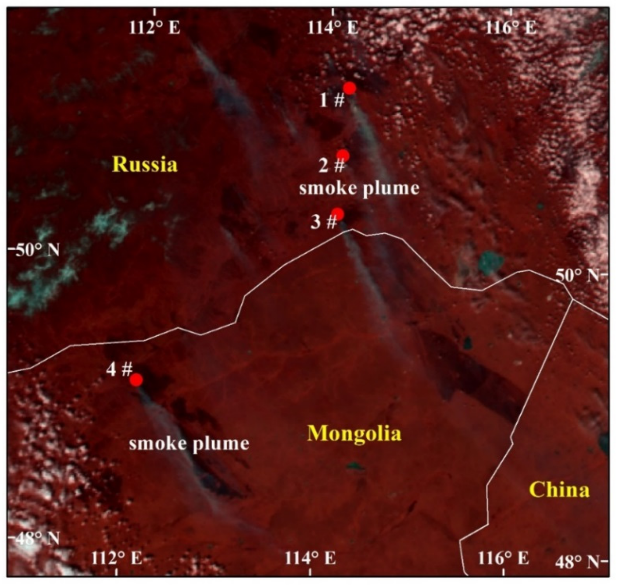
We targeted wildfires covered by Aqua MODIS images and OCO-2 on the same day where OCO-2 points must intersect wildfire smoke plumes. The MODIS products of MCD64A1 and Landsat images were used to obtain wildfire information. Then, we downloaded the Aqua MODIS L1B images covering the wildfires and identified smoke plumes visually. Based on the time span of wildfires and spatial range of smoke plumes, OCO-2 L2 data covering smoke plumes were downloaded to look for the intersect points. We selected one wildfire that met our standard in Siberia (on 20 April 2015), the cross time was 20 April 2015 05:13:08 and 20 April 2015 05:15:00 LT for OCO-2 and Aqua MODIS, respectively (Figure 1).
2.5. CO2 Emission Method (OCO-2 Model)
In this study, we are going to explore a new method to quantify the CO2 released from wildfires that is based on the transitional equation of mass calculation as shown below:
ECO2 = ρ × V
ECO2 indicates CO2 emissions from wildfire, ρ is the density of CO2, and V is the volume of smoke plumes calculated using S (area) and multiplied by H (height). S is the area of smoke plumes calculated from MODIS images and H is the height of smoke plumes, which will be derived using MINX. The equation can thus be expressed as follows:
ECO2 =ρ × S × H
As shown before, the unit of OCO-2 XCO2 data is parts per million (ppm). To calculate the quantity of CO2 released from wildfires, it was necessary to convert these numbers to density values using
ρ = M/22.4 × ppm × (273/T) × (Ba/1013.25)
2.6. Biomass Burning Model (BBM)
BBM [9,41] has been widely used to evaluate trace gas emission from wildfires and for studying the release of trace gases from biomass burning [55,56,57]. It is calculated based on the conservation of mass:
where Es (Mg) is CO2 emissions from wildfires, S is the burned area (ha) as indicated from satellite images, B is the biomass fuel load (Mg ha−1), β is the combustion factor (%), and EF is the emission factor of CO2 (kg kg−1).
Es = S × B × β × EF
Many researchers used different approaches to obtain the BBM parameter for different ecological systems [13,56,58]. Among them, Akagi, et al. [59] summarized much of the literature data for biomass consumption for different vegetation and fire types, and in this paper we used the parameter of Akagi, et al. [59] to calculate CO2 emissions which were used to verify the accuracy of OCO-2 model.
3. Results
3.1. Smoke Plume Area Detection and Height Derivation
To calculate CO2 emissions from wildfires, we must know smoke plume characteristics such as height, distribution, and the value of XCO2. First, smoke plumes from wildfire must be detected accurately. Remote-sensing data can accomplish this work quite well and MODIS data were suitable for this study. Using the threshold of MODIS band 8, we detected the smoke plumes of the 4 fire cases (Figure 2) with area of 2.48 × 10³ km2, 2.41 × 10³ km2, 2.50 × 10³ km2 and 6.48 × 10³ km2, respectively.
As mentioned above, MINX has the potential to extract smoke characteristics and here we combine MINX and MODIS data to identify smoke plumes. By employing MINX v4.0, we derived the height of each wildfire smoke plume (Figure 3). We calculated the average height of each smoke plume pixel and obtained the height value as 2.29 km, 2.38 km, 1.99 km, and 2.61 km for the 4 smoke plumes, respectively.
From MINX results we can also obtain the smoke plume area of 1.46 × 10³ km2, 1.31 × 10³ km2, 1.36 × 10³ km2, and 1.04 × 10³ km2, respectively which are rather lower than that from MODIS band 8. MINX was robust in deriving aerosol height but could only recognize thick smoke which could be easily identified from true color images. MODIS band 8 has the potential to derive thin smokes using the reflectance threshold.
3.2. Burned Area Monitor
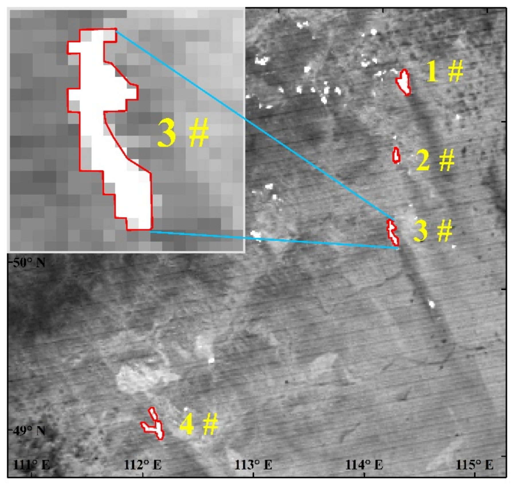
Burned area of forest fires could be accurately and rapidly monitored using remote-sensing images based on sharp differences in the spectral characteristics of the surface inside and outside of the burned scars. Using MODIS band 21 (MYD021KM.A2015110.0515.006.2015110190452) fire points were observed and visual interpretation was used to map the burned scars (Figure 4). Here, we assume that the smoke plumes were released from the mapped burned scars. Given that the spatial resolution of MODIS is 1000 m, the burned scars must contain many mixed pixels. This means that the burned areas used in this study are worth discussion.
3.3. Model XCO2 from Smoke Plumes
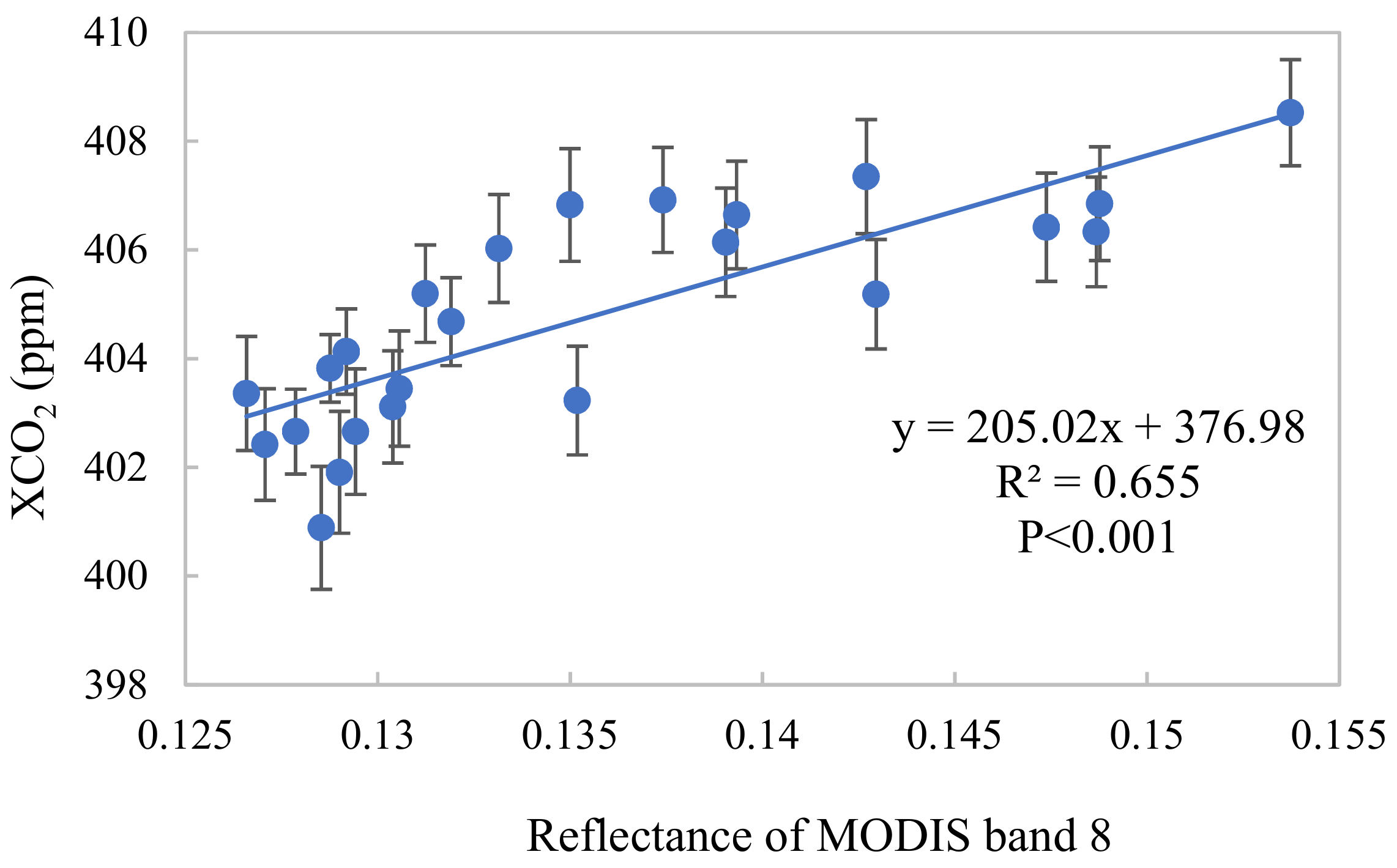
The XCO2 values of smoke plume pixels changed with the smoke concentration. To calculate CO2 emissions accurately, we first calculated XCO2 values for each smoke plume pixel and then subtracted clear sky XCO2 values. In this paper, linear regression analysis was used based on OCO-2 XCO2 values and MODIS band 8 reflectance in the intersection regions. Scatter plots of XCO2 against MODIS band 8 reflectance in the study region are shown in Figure 4 and close correlations were found (R2 = 0.655, p < 0.001). By using the relationships between MODIS band 8 reflectance and XCO2, we could calculate XCO2 of the smoke plume pixels that did not intersect with OCO-2 points (Figure 5). In Figure 6 we see that XCO2 also has different values because of differences in smoke concentration. Higher values are in the center, and lower values are at the edges of the smoke plumes. XCO2 values decreased with increasing transport distance.
3.4. CO2 Emission Calculation from OCO-2 Model
Equations 1–3 (named the OCO-2 model) were used to calculate CO2 emissions from wildfires. In the OCO-2 model, the height of the smoke plumes was derived from MISR data using MINX v4.0 software, the smoke plumes were derived from MODIS band 8. The calculated CO2 emissions for each fire point are shown in Table 1. We found that CO2 emissions were from 122.21 (±4.87) × 103 Mg for the 2# wildfire to 288.70 (±14.33) × 103 Mg for the 4# wildfire.
4. Discussion
4.1. Smoke Plume Height Estimation
Energy from wildfires, especially crown fire, can loft smoke plumes above the boundary layer and promote long-distance transport of gases and particulate matter. Not all smoke aerosols rise high enough and form plumes. A great number of smoke aerosols remain in the near-ground layer [4,49].
From OCO-2 model we know that the height of smoke plume is rather important in determining the accuracy of CO2 emissions. Regarding the height of smoke plumes, researchers acquire different results using different methods for different fires. Vadrevu, et al. [60] used Cloud-Aerosol Lidar and Infrared Pathfinder Satellite Observations (CALIPSO) to monitor the mean smoke height and suggested that the value was from 2.5 to 9.3 km with an average height of 5.35 km at the northern border of India. Using multi-wavelength lidar, MODIS, and CALIOP imageries, Wu, et al. [61] obtained different elevation values of smoke plumes from 1.5 to 6.5 km for different fire case locations. Ross, et al. [41] assumed the plume height was 0.3, 1, 2, and 5 km to assess the ratio of XCO2 and XCH4 from GOSAT in the presence of wildfire plumes. Guo, et al. [7] used GOSAT FTS-TIR L2 data to identify the boundary of smoke plumes in a Russian wildfire of 2010 and obtained the height of 1.58 km; however, this result warrants discussion because of the coarse resolution of GOSAT profile data. Kahn, et al. [50] calculated the height of smoke plumes in Australia using the Multi-angle Imaging SpectroRadiometer (MISR) instrument and found wind-corrected values of approximately 3.5 km. Mazzoni, et al. [49] employed MISR and MODIS data collected over North America during the summer of 2004 and found that the plume height was approximately 3 km (see Figure 5 in Mazzoni, et al. [49]).
By employing MINX v4.0, we calculated the height of each wildfire smoke plume as shown in Figure 3. To simplify, we calculated the average height of each smoke plume pixel and obtained the height value as 2.29 km, 2.38 km, 1.99 km, and 2.61 km respectively for the 4 smoke plumes. Compared with former research, we found that our results were slightly lower for the average smoke plume height which is mainly due to lower energy released from small burned areas.
4.2. CO2 Emissions by BBM
Using OCO-2 model, we have estimated CO2 releases from 4 fire scars in Siberia. As we have shown, this is the first time that there has been a determination of CO2 emissions from forest fires using OCO-2 data. We employed BBM, the most commonly used method in estimating trace gases emission from biomass burning [11,13,21], to verify the accuracy of our results.
As mentioned above, it is difficult and complex to obtain these variables accurately because of the high spatial heterogeneity of vegetation, different weather conditions, and different behaviors of each fire [7,14]. It is also quite difficult for us to field measure all these variables in Siberia by ourselves. Luckily, each variable, such as biomass fuel load, combustion factor, and EF, have been discussed by many researchers in recent years. Based on the former researchers’ results, Werf, et al. [13] argued that the EF in an extratropical forest was 1572 g kg−1. Based on localized measurements, Zhou, et al. [16] found that the EF was 1543-1630 g kg−1 in Chinese forests. The study by Shi and Yamaguchi [15] found an EF of 1580 g kg−1 in the forests of Southeast Asia. Chang and Song [56] used an EF value of 1618 g kg−1 for the forest to estimate biomass burning emissions in tropical Asia. Akagi, et al. [59] used emission ratios (the molar ratio between the two emitted compounds) to derive EF based on the carbon mass balance method. Laboratory- and ground-based measurements and airborne measurements of EF for burning organic soils, peat, and woody/down/dead vegetation by many researchers were considered in order to calculate EF by Akagi, et al. [59], who concluded that the EF of CO2 for boreal forests is 1.489 (±0.121) kg kg−1. The study region in this work is located at high latitudes where the most important boreal forests in the world exist which is similar with Akagi et al.’s research. Thus, in this paper, we used the EF of 1.489 (±0.121) kg kg−1.
Akagi, et al. [59] summarized much of the literature data for biomass consumption (biomass loading multiply combustion factor) for different vegetation and fire types and we used their result of 38 Mg ha−1 here.
CO2 emissions from each fire scar and all other variables are shown in Table 2. The comparisons with the results of the OCO-2 model are also listed. We found that the results by the BBM are higher than those of the OCO-2 model for all 4 fire scars. The most similar results were found in the second fire scar (25.76%); the largest bias was in the first fire scar (157.11%) followed by the third (121.10%). We found that all of the study cases have an equal magnitude of CO2 emission results by the BBM and OCO-2 models. Thus, we can propose that OCO-2 has great potential in estimating CO2 emissions from wildfires.
4.3. CO2 Emission Differences between the Two Models
Table 2 show the different CO2 releases from boreal forest fires between BBM and OCO-2 models. We found that the BBM results are higher than those of the OCO-2 (from 25.76% to 157.11%) but remain within our expected range.
The differences may be due to the uncertainty variables of BBM. The biomass fuel load and combustion factors are crucial but difficult to estimate accurately. Biomass fuel load estimates are complex because of the high spatial heterogeneity of the different types of vegetation sampled. Biomass fuel load (here, we just consider the aboveground biomass) was calculated at three levels: litter, surface fuels, and tree crowns; all these three levels change with species and vegetation type and are also affected by the age structure of the forest, the years since the last disturbance, and so on [14,41]. Saatchi, et al. [62] found that the error of forest biomass fuel load is about 50%. The boreal forest is made up by many different biological communities with different biomass loads. The burned scars, especially the larger ones, usually contain many biological communities. The study region is located at the edge of Siberia and the vegetation communities may differ with former research. In this paper, we did not consider biological communities and used one value for the study region. Biomass fuel load based on vegetation community information may increase the estimation accuracy.
Another variable that affected the BBM result is combustion factor, which indicates the ratio of the burned biomass during a fire and is also difficult to estimate because of differences in vegetation characteristics (i.e., plant age, growth cycle, and water content), as well as the unique behavior of each fire. Many researchers have argued that the combustion factor is affected by fire type (surface fire, crown fire, or ground fire), fire phase (flaming or smoldering), and many other factors, such as wind speed, month of occurrence (vegetation has different water content in spring and summer), soil moisture, and even different slope aspects; the different regions ranges of the combustion factor are from 34%~69% with an uncertainty of 50% [7,13,56,59,63]. Uncertainties over the emission factor can also not be ignored and researchers obtained different EF values for boreal forests [13,59].
Burned area is also an important factor that affects CO2 emissions. CO2 emissions from forest fires have a strong correlation with burned area; accurate measurement of burned area has been crucial for CO2 emission estimates [14]. Post-fire burned area could be fairly accurately mapped by airborne and satellite imageries of boreal forests but in this paper, the burned areas were not the post-fire areas. Due to the higher reflectance of burning biomass the burned area may be enlarged in this study. We looked at actively burning forest and freshly burned areas that could correspond with smoke plumes, meaning we could not use any other higher spatial-resolution images aside from those of Aqua MODIS.
Uncertainties in the OCO-2 model may come from the smoke plume area, the modeled XCO2 value of each pixel, as well as the bias of OCO-2 retrieval XCO2 values. In this study, the smoke plumes were identified by the thresholds of MODIS band 8 which were affected by the researcher’s knowledge of remote sensing.
O’Dell, et al. [64] argued that the retrieval XCO2 will lead to a small positive bias of about 0.3 ppm when thin cirrus appears. They also defined the clouds as the aerosol optical depth (AOD) greater than 0.3. In this study we used MODIS product (MYD04, version 061) with a spatial resolution of 3 km to view the AOD value of wildfire smoke plumes that overlaid with the OCO-2 footprint. We found that all the AOD values of smoke plumes used for the XCO2 model were lower than 0.3 which means that we could ignore this bias. With the increasing AOD of smoke plumes, the modeled XCO2 bias may increase; here we did not consider this error. Thermal Infrared Red (TIR) satellite soundings have low sensitivity below 2–3 km of altitude, especially in the boundary layer [65], therefore OCO-2 retrieved XCO2 may be underestimated in the smoke plumes boundary layer. We also did not consider this bias in this paper.
4.4. Advantages and Limitations of the OCO-2 Model
The OCO-2 model calculates CO2 emissions using the △XCO2 value and smoke plume characteristics that can be obtained using remote-sensing techniques. It has the advantage of remote-sensing technologies repeat data acquisition, such as being more efficient and saving labor costs.
However, there are limitations for the OCO-2 model. Firstly, there may be an error when smoke plumes area is identified. The threshold of the smoke plume area identified was based on artificial visual interpretations, and the accuracy depended on the knowledge and understanding of smoke plume characteristics by researchers. Although MISR data could be used as a reference, some smoke plumes, especially the smoke released from earlier burning, will be dispersed into the atmosphere and could not be captured by the MODIS sensor. To some extent, this could explain why the estimated CO2 emissions using the OCO-2 model are lower than BBM.
Secondly, the most serious limitation of our approach is the lack of data. Given the 16-day recycle time of OCO-2, it is not easy to intersect with the smoke plumes, meaning that smoke from small or short-lived wildfires could not be captured by the OCO-2 satellite. It is time consuming to look for OCO-2 points that intersect MODIS smoke plumes on the same day. In this study, we just attempt to explore a simple and accurate method for using remote sensing data to estimate CO2 emissions from wildfires and in the future, automatic methods for identifying smoke plumes and selecting the intersected OCO-2 points must be developed.
5. Conclusions
Every year, thousands of wildfires occur in boreal forests and release a great amount of CO2 into the atmosphere. Wildfires transform forests from carbon sinks into sources. Accurate estimation of GHG, especially CO2 from wildfire in boreal forests, is necessary to understand the role of boreal forests in carbon cycle and global warming. This study explored the feasibility of using OCO-2 and MODIS data to estimate CO2 emissions from wildfires in boreal forests and we were able to draw a few conclusions.
Firstly, CO2 emissions could be calculated using OCO-2 data and Aqua MODIS images because of the close passing time over the same territories. MODIS band 8 and 21 could be used in smoke plume identification and burned area monitoring. Because of the higher reflectance of burning biomass, the burned area identified in this study may be enlarged and lead to higher CO2 emissions from BBM.
Secondly, the widely used biomass burning method, BBM, was used to verify the results of the OCO-2 model and found that the biases were between 25.76% and 157.11%. The different results between BBM and the OCO-2 model were because of the biases of the smoke plumes area, smoke plume height, burned area, biomass fuel load, and even the different biological communities of the study region with the references.
Thirdly, based on the different CO2 emission results, the advantages and limitations of the OCO-2 model in estimating CO2 emissions from wildfires were analyzed and found that OCO-2 is a useful tool for fire-emission monitoring.
The present study proposed a new approach to estimate CO2 emissions from wildfires using remote-sensing data and extends the application range of GHG satellites. In the future, many works are needed to perfect the OCO-2 model, especially to improve its efficiency and accuracy.
Author Contributions
Methodology, M.G.; software, L.W.; formal analysis, S.H.; writing—original draft preparation, M.G. and J.L.; writing—review and editing, M.G. and J.L.; funding acquisition, J.L., M.G.
Funding
This research was funded by the National Natural Science Foundation of China (41871103 and 41771179) and the National Key Research and Development Project (2016YFA0602301).
Acknowledgments
We would like to thank the NASA Goddard Earth Science Data and Information Services Center for the use of OCO-2 data in this study. We also would like to thank MISR data of NASA and the MINX v4.0 software of California Institute of Technology.
Conflicts of Interest
The authors declare that there is no conflict of interest.
References
- Williams, C.A.; Gu, H.; MacLean, R.; Masek, J.G.; Collatz, G.J. Disturbance and the carbon balance of us forests: A quantitative review of impacts from harvests, fires, insects, and droughts. Glob. Planet. Chang. 2016, 143, 66–80. [Google Scholar] [CrossRef]
- Boby, L.A.; Schuur, E.A.G.; Mack, M.C.; Verbyla, D.; Johnstone, J.F. Quantifying fire severity, carbon, and nitrogen emissions in Alaska’s boreal forest. Ecol. Appl. 2010, 20, 1633–1647. [Google Scholar] [CrossRef] [PubMed]
- Van Marle, M.J.E.; Kloster, S.; Magi, B.I.; Marlon, J.R.; Daniau, A.L.; Field, R.D.; Arneth, A.; Forrest, M.; Hantson, S.; Kehrwald, N.M.; et al. Historic global biomass burning emissions for CMIP6 (BB4CMIP) based on merging satellite observations with proxies and fire models (1750–2015). Geosci. Model Dev. 2017, 10, 3329–3357. [Google Scholar] [CrossRef]
- Fisher, D.; Muller, J.P.; Yershov, V.N. Automated stereo retrieval of smoke plume injection heights and retrieval of smoke plume masks from aatsr and their assessment with CALIPSO and MISR. IEEE Trans. Geosci. Remote Sens. 2014, 52, 1249–1258. [Google Scholar] [CrossRef]
- Langner, A.; Siegert, F. Spatiotemporal fire occurrence in Borneo over a period of 10 years. Glob. Chang. Biol. 2009, 15, 48–62. [Google Scholar] [CrossRef]
- Alexander, H.D.; Mack, M.C. A canopy shift in interior Alaskan boreal forests: Consequences for above- and belowground carbon and nitrogen pools during post-fire succession. Ecosystems 2016, 19, 98–114. [Google Scholar] [CrossRef]
- Guo, M.; Li, J.; Xu, J.; Wang, X.; He, H.; Wu, L. CO2 emissions from the 2010 russian wildfires using gosat data. Environ. Pollut. 2017, 226, 60–68. [Google Scholar] [CrossRef] [PubMed]
- Virkkula, A.; Levula, J.; Pohja, T.; Aalto, P.P.; Keronen, P.; Schobesberger, S.; Clements, C.B.; Pirjola, L.; Kieloaho, A.J.; Kulmala, L.; et al. Prescribed burning of logging slash in the boreal forest of Finland: Emissions and effects on meteorological quantities and soil properties. Atmos. Chem. Phys. 2014, 14, 4473–4502. [Google Scholar] [CrossRef]
- Seiler, W.; Crutzen, P.J. Estimates of gross and net fluxes of carbon between the biosphere and the atmosphere from biomass burning. Clim. Chang. 1980, 2, 207–247. [Google Scholar] [CrossRef]
- Miranda, A.I.; Coutinho, M.; Borrego, C. Forest fire emissions in Portugal: A contribution to global warming? Environ. Pollut. 1994, 83, 121–123. [Google Scholar] [CrossRef]
- Wiedinmyer, C.; Neff, J.C. Estimates of CO2 from fires in the United States: Implications for carbon management. Carbon Balance Manag. 2007, 2, 10. [Google Scholar] [CrossRef] [PubMed]
- Barbosa, P.; Camia, A.; Kucera, J.; Libertà, G.; Palumbo, I.; San-Miguel-Ayanz, J.; Schmuck, G. Chapter 8 Assessment of Forest Fire Impacts and Emissions in the European Union Based on the European Forest Fire Information System; Elsevier Science & Technology: Amsterdam, The Netherlands, 2008; pp. 197–208. [Google Scholar]
- Van der Werf, G.R.; Randerson, J.T.; Giglio, L.; Collatz, G.J.; Mu, M.; Kasibhatla, P.S.; Morton, D.C.; Defries, R.S.; Jin, Y.; Leeuwen, T.T.V. Global fire emissions and the contribution of deforestation, savanna, forest, agricultural, and peat fires (1997–2009). Atmos. Chem. Phys. 2010, 10, 16153–16230. [Google Scholar] [CrossRef]
- Rosa, I.M.D.; Pereira, J.M.C.; Tarantola, S. Atmospheric emissions from vegetation fires in Portugal (1990–2008): Estimates, uncertainty analysis, and sensitivity analysis. Atmos. Chem. Phys. 2011, 11, 2625–2640. [Google Scholar] [CrossRef]
- Shi, Y.; Yamaguchi, Y. A high-resolution and multi-year emissions inventory for biomass burning in Southeast Asia during 2001–2010. Atmos. Environ. 2014, 98, 8–16. [Google Scholar] [CrossRef]
- Zhou, Y.; Xing, X.; Lang, J.; Chen, D.; Cheng, S.; Wei, L.; Wei, X.; Liu, C. A comprehensive biomass burning emission inventory with high spatial and temporal resolution in China. Atmos. Chem. Phys. 2017, 17, 2839–2864. [Google Scholar] [CrossRef] [Green Version]
- Pereira, G.; Freitas, S.R.; Moraes, E.C.; Ferreira, N.J.; Shimabukuro, Y.E.; Rao, V.B.; Longo, K.M. Estimating trace gas and aerosol emissions over South America: Relationship between fire radiative energy released and aerosol optical depth observations. Atmos. Environ. 2009, 43, 6388–6397. [Google Scholar] [CrossRef]
- Liu, M.; Song, Y.; Yao, H.; Kang, Y.; Li, M.; Huang, X.; Hu, M. Estimating emissions from agricultural fires in the North China Plain based on MODIS fire radiative power. Atmos. Environ. 2015, 112, 326–334. [Google Scholar] [CrossRef]
- Wooster, M.J.; Freeborn, P.H.; Archibald, S.; Oppenheimer, C.; Roberts, G.J.; Smith, T.E.L.; Govender, N.; Burton, M.; Palumbo, I. Field determination of biomass burning emission ratios and factors via open-path ftir spectroscopy and fire radiative power assessment: Headfire, backfire and residual smouldering combustion in African savannahs. Atmos. Chem. Phys. 2011, 11, 11591–11615. [Google Scholar] [CrossRef]
- Kaiser, J.W.; Heil, A.; Andreae, M.O.; Benedetti, A.; Chubarova, N.; Jones, L.; Morcrette, J.J.; Razinger, M.; Schultz, M.G.; Suttie, M. Biomass burning emissions estimated with a global fire assimilation system based on observed fire radiative power. Biogeosci. Discuss. 2012, 9, 527–554. [Google Scholar] [CrossRef] [Green Version]
- Konovalov, I.B.; Berezin, E.V.; Ciais, P.; Broquet, G.; Beekmann, M.; Hadjilazaro, J.; Clerbaux, C.; Andreae, M.O.; Kaiser, J.W.; Schulze, E.D. Constraining CO2 emissions from open biomass burning by satellite observations of co-emitted species: A method and its application to wildfires in Siberia. Atmos. Chem. Phys. 2014, 14, 10383–10410. [Google Scholar] [CrossRef]
- Konovalov, I.B.; Beekmann, M.; Berezin, E.V.; Formenti, P.; Andreae, M.O. Probing into the aging dynamics of biomass burning aerosol by using satellite measurements of aerosol optical depth and carbon monoxide. Atmos. Chem. Phys. 2016, 17, 4513–4537. [Google Scholar] [CrossRef]
- Mu, M.; Randerson, J.T.; Van der Werf, G.R.; Giglio, L.; Kasibhatla, P.; Morton, D.; Collatz, G.J.; Defries, R.S.; Hyer, E.J.; Prins, E.M. Daily and 3-hourly variability in global fire emissions and consequences for atmospheric model predictions of carbon monoxide. J. Geophys. Res. Atmos. 2011, 116, 24303. [Google Scholar] [CrossRef]
- Wiedinmyer, C.; Akagi, S.K.; Yokelson, R.J.; Emmons, L.K. The Fire INventory from NCAR (FINN)—A high resolution global model to estimate the emissions from open burning. Geosci. Model Dev. Discuss. 2011, 3, 625–641. [Google Scholar] [CrossRef]
- Kaiser, J.W.; Flemming, J.; Schultz, M.G.; Suttie, M.; Wooster, M.J. The MACC Global Fire Assimilation System: First emission products (GFASv0). ECMWF Tech. Memo. 2009, 596, 1–6. [Google Scholar]
- Arnett, J.T.; Coops, N.C.; Daniels, L.D.; Falls, R.W. Detecting forest damage after a low-severity fire using remote sensing at multiple scales. Int. J. Appl. Earth Obs. Geoinf. 2015, 35, 239–246. [Google Scholar] [CrossRef]
- Heymann, J.; Reuter, M.; Buchwitz, M.; Schneising, O.; Bovensmann, H.; Burrows, J.P.; Massart, S.; Kaiser, J.W.; Crisp, D. CO2 emission of indonesian fires in 2015 estimated from satellite-derived atmospheric CO2 concentrations. Geophys. Res. Lett. 2017, 44, 1537–1544. [Google Scholar] [CrossRef]
- Patra, P.K.; Crisp, D.; Kaiser, J.W.; Wunch, D.; Saeki, T.; Ichii, K.; Sekiya, T.; Wennberg, P.O.; Feist, D.G.; Pollard, D.F. The orbiting carbon observatory (OCO-2) tracks 2–3 peta-gram increase in carbon release to the atmosphere during the 2014–2016 EI Nino. Sci. Rep. 2017, 7, 13567. [Google Scholar] [CrossRef]
- Connor, B.; Bösch, H.; McDuffie, J.; Taylor, T.; Fu, D.; Frankenberg, C.; O’Dell, C.; Payne, V.H.; Gunson, M.; Pollock, R.; et al. Quantification of uncertainties in OCO-2 measurements of XCO2: Simulations and linear error analysis. Atmos. Meas. Tech. 2016, 9, 5227–5238. [Google Scholar] [CrossRef]
- Wunch, D.; Wennberg, P.O.; Osterman, G.; Fisher, B.; Naylor, B.; Roehl, C.M.; O’Dell, C.; Mandrake, L.; Viatte, C.; Kiel, M. Comparisons of the Orbiting Carbon Observatory-2 (OCO-2) XCO2 measurements with TCCON. Atmos. Meas. Tech. 2017, 10, 1–45. [Google Scholar] [CrossRef]
- Crisp, D.; Pollock, H.; Rosenberg, R.; Chapsky, L.; Lee, R.; Oyafuso, F.; Frankenberg, C.; Dell, C.; Bruegge, C.; Doran, G.; et al. The on-orbit performance of the Orbiting Carbon Observatory-2 (OCO-2) instrument and its radiometrically calibrated products. Atmos. Meas. Tech. 2017, 10, 59–81. [Google Scholar] [CrossRef] [Green Version]
- Pollock, R.; Haring, R.E.; Holden, J.R.; Johnson, D.L.; Kapitanoff, A.; Mohlman, D.; Phillips, C.; Randall, D.; Rechsteiner, D.; Rivera, J.; et al. The orbiting carbon observatory instrument: Performance of the oco instrument and plans for the OCO-2 instrument. In Proceedings of the SPIE—The International Society for Optical Engineering, Toulouse, France, 13 October 2010. [Google Scholar]
- Prasad, P.; Rastogi, S.; Singh, R.P.; Panigrahy, S. Spectral modelling near the 1.6 μm window for satellite based estimation of CO2. Spectrochim. Acta A Mol. Biomol. Spectrosc. 2014, 117, 330–339. [Google Scholar] [CrossRef] [PubMed]
- Lee, R.A.M.; O’Dell, C.W.; Wunch, D.; Roehl, C.M.; Osterman, G.B.; Blavier, J.F.; Rosenberg, R.; Chapsky, L.; Frankenberg, C.; Hunyadi-Lay, S.L.; et al. Preflight spectral calibration of the Orbiting Carbon Observatory 2. IEEE Trans. Geosci. Remote Sens. 2017, 55, 2499–2508. [Google Scholar] [CrossRef]
- Day, J.O.; O’Dell, C.W.; Pollock, R.; Bruegge, C.J.; Rider, D.; Crisp, D.; Miller, C.E. Preflight spectral calibration of the orbiting carbon observatory. In Proceedings of the International Conference on Next Generation Mobile Applications, Amman, Jordan, 27–29 July 2010; pp. 13–18. [Google Scholar]
- Frankenberg, C.; Pollock, R.; Lee, R.A.M.; Rosenberg, R.; Blavier, J.F.; Crisp, D.; O’Dell, C.W.; Osterman, G.B.; Roehl, C.; Wennberg, P.O.; et al. The Orbiting Carbon Observatory (OCO-2): Spectrometer performance evaluation using pre-launch direct sun measurements. Atmos. Meas. Tech. 2015, 8, 301–313. [Google Scholar] [CrossRef]
- Meng, J.; Ding, G.; Liu, L.; Zhang, R. A comparison and validation of atmosphere CO2 concentration OCO-2-based observations and tccon-based observations. In Communications in Computer and Information Science; Springer: Singapore, 2016; Volume 645, pp. 356–363. [Google Scholar]
- Eldering, A.; O’Dell, C.W.; Wennberg, P.O.; Crisp, D.; Gunson, M.R.; Viatte, C.; Avis, C.; Braverman, A.; Castano, R.; Chang, A.; et al. The Orbiting Carbon Observatory-2: First 18 months of science data products. Atmos. Meas. Tech. 2017, 10, 549–563. [Google Scholar] [CrossRef]
- Mandrake, L.; Frankenberg, C.; O’Dell, C.W.; Osterman, G.; Wennberg, P.; Wunch, D. Semi-autonomous sounding selection for OCO-2. Atmos. Meas. Tech. 2013, 6, 2851–2864. [Google Scholar] [CrossRef] [Green Version]
- Ross, A. Gosat Measurements of Wildfire Emissions; University of London: London, UK, 2012. [Google Scholar]
- Ross, A.N.; Wooster, M.J.; Boesch, H.; Parker, R. First satellite measurements of carbon dioxide and methane emission ratios in wildfire plumes. Geophys. Res. Lett. 2013, 40, 4098–4102. [Google Scholar] [CrossRef] [Green Version]
- Chand, T.R.K.; Badarinath, K.V.S.; Murthy, M.S.R.; Rajshekhar, G.; Elvidge, C.D.; Tuttle, B.T. Active forest fire monitoring in Uttaranchal State, India using multi-temporal DMSP-OLS and MODIS data. Int. J. Remote Sens. 2007, 28, 2123–2132. [Google Scholar] [CrossRef]
- Guo, M.; Li, J.; Sheng, C.; Xu, J.; Li, W. A review of wetland remote sensing. Sensors 2017, 17, 777. [Google Scholar] [CrossRef]
- Roy, D.; Descloitres, J.; Alleaume, S. The MODIS fire products. Remote Sens. Environ. 2002, 83, 244–262. [Google Scholar]
- Cheng, D.; Rogan, J.; Schneider, L.; Cochrane, M. Evaluating MODIS active fire products in subtropical yucatán forest. Remote Sens. Lett. 2013, 4, 455–464. [Google Scholar] [CrossRef]
- Chen, D.; Pereira, J.M.C.; Masiero, A.; Pirotti, F. Mapping fire regimes in China using MODIS active fire and burned area data. Appl. Geogr. 2017, 85, 14–26. [Google Scholar] [CrossRef]
- Ganci, G.; Negro, C.D.; Fortuna, L.; Vicari, A. A tool for multi-platform remote sensing processing. Commun. Simai Congr. 2009, 3, 281. [Google Scholar]
- Wan, Z.; Ng, D.; Dozier, J. Spectral emissivity measurements of land-surface materials and related radiative transfer simulations. Adv. Space Res. 1994, 14, 91–94. [Google Scholar] [CrossRef]
- Mazzoni, D.; Logan, J.A.; Diner, D.; Kahn, R.; Tong, L.; Li, Q. A data-mining approach to associating MISR smoke plume heights with MODIS fire measurements. Remote Sens. Environ. 2007, 107, 138–148. [Google Scholar] [CrossRef]
- Kahn, R.A.; Moroney, C.M.; Gaitley, B.J.; Nelson, D.L.; Garay, M.J.; Mims, S.R. MISR stereo heights of grassland fire smoke plumes in Australia. IEEE Trans. Geosci. Remote Sens. 2009, 48, 25–35. [Google Scholar]
- Gonzalez, L.; Val Martin, M.; Kahn, R. Biomass burning smoke heights over the Amazon observed from space. Atmos. Chem. Phys. 2019, 19, 1685–16702. [Google Scholar] [CrossRef]
- Nelson, D.L.; Garay, M.J.; Kahn, R.A.; Dunst, B.A. Stereoscopic height and wind retrievals for aerosol plumes with the MISR INteractive eXplorer (MINX). Remote Sens. 2013, 5, 4593–4628. [Google Scholar] [CrossRef]
- Sofiev, M.; Ermakova, T.; Vankevich, R. Evaluation of the smoke-injection height from wild-land fires using remote-sensing data. Atmos. Chem. Phys. 2012, 11, 27937–27966. [Google Scholar] [CrossRef]
- Kahn, R.A.; Li, W.H.; Moroney, C.; Diner, D.J.; Martonchik, J.V.; Fishbein, E. Aerosol source plume physical characteristics from space-based multiangle imaging. J. Geophys. Res. Atmos. 2007, 112, 1–20. [Google Scholar]
- Goto, Y.; Suzuki, S. Estimates of carbon emissions from forest fires in Japan, 1979–2008. Int. J. Wildland Fire 2013, 22, 721–729. [Google Scholar] [CrossRef]
- Chang, D.; Song, Y. Estimates of biomass burning emissions in tropical Asia based on satellite-derived data. Atmos. Chem. Phys. 2010, 10, 2335–2351. [Google Scholar] [CrossRef] [Green Version]
- Shi, Y.; Matsunaga, T.; Yamaguchi, Y. High-resolution mapping of biomass burning emissions in three tropical regions. Environ. Sci. Technol. 2015, 49, 10806–10814. [Google Scholar] [CrossRef] [PubMed]
- Shi, Y.; Sasai, T.; Yamaguchi, Y. Spatio-temporal evaluation of carbon emissions from biomass burning in Southeast Asia during the period 2001–2010. Ecol. Model. 2014, 272, 98–115. [Google Scholar] [CrossRef]
- Akagi, S.K.; Yokelson, R.J.; Wiedinmyer, C.; Alvarado, M.J.; Reid, J.S.; Karl, T.; Crounse, J.D.; Wennberg, P.O. Emission factors for open and domestic biomass burning for use in atmospheric models. Atmos. Chem. Phys. 2011, 11, 4039–4072. [Google Scholar] [CrossRef] [Green Version]
- Vadrevu, K.; Ellicott, E.; Giglio, L.; Badarinath, K.V.S.; Vermote, E.; Justice, C.; Lau, W. Vegetation fires in the himalayan region—aerosol load, black carbon emissions and smoke plume heights. Atmos. Environ. 2012, 47, 241–251. [Google Scholar] [CrossRef]
- Wu, Y.; Cordero, L.; Gross, B.; Moshary, F.; Ahmed, S. Smoke plume optical properties and transport observed by a multi-wavelength lidar, sunphotometer and satellite. Atmos. Environ. 2012, 63, 32–42. [Google Scholar] [CrossRef]
- Saatchi, S.S.; Harris, N.L.; Brown, S.; Lefsky, M.; Mitchard, E.T.; Salas, W.; Zutta, B.R.; Buermann, W.; Lewis, S.L.; Hagen, S. Benchmark map of forest carbon stocks in tropical regions across three continents. Proc. Natl. Acad. Sci. USA 2011, 108, 9899. [Google Scholar] [CrossRef] [PubMed]
- Kauffman, J.B.; Steele, M.D.; Cummings, D.L.; Jaramillo, V.J. Biomass dynamics associated with deforestation, fire, and conversion to cattle pasture in a Mexican tropical dry forest. For. Ecol. Manag. 2003, 176, 1–12. [Google Scholar] [CrossRef]
- O’Dell, C.W.; Connor, B.; Bösch, H.; O’Brien, D. The ACOS CO2 retrieval algorithm—Part 1: Description and validation against synthetic observations. Atmos. Meas. Tech. 2011, 4, 99–121. [Google Scholar]
- Yurganov, L.N.; Rakitin, V.; Dzhola, A.; August, T.; Fokeeva, E.; George, M.; Gorchakov, G.; Grechko, E.; Hannon, S.; Karpov, A. Satellite- and ground-based CO total column observations over 2010 Russian fires: Accuracy of top-down estimates based on thermal IR satellite data. Atmos. Chem. Phys. Discuss. 2011, 11, 7925–7942. [Google Scholar] [CrossRef]
Figure 1.
Moderate-resolution Imaging Spectroradiometer (MODIS) false-color image (red-green-blue (RGB) = 741) of study region. The white lines indicate national boundaries and the red point is fire point. Smoke plumes can be identified from the image. We found 3 active fires in Russia and 1 in Mongolia, but here, the study region is labeled “Siberia”.

Figure 2.
Smoke plumes detection using MODIS band 8.
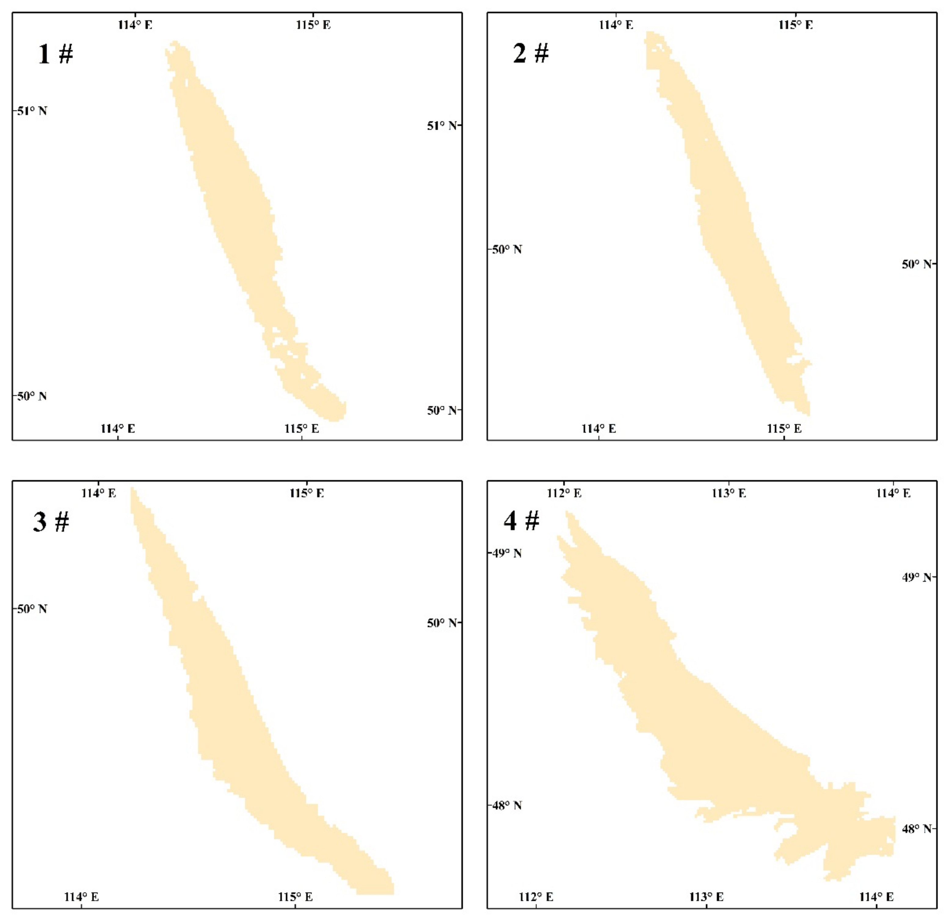
Figure 3.
Height of smoke plume sketches derived from Multi-Angle Imaging Spectroradiometer (MISR) data by employing MISR Interactive Explorer (MINX) v4.0 software.
Figure 3.
Height of smoke plume sketches derived from Multi-Angle Imaging Spectroradiometer (MISR) data by employing MISR Interactive Explorer (MINX) v4.0 software.
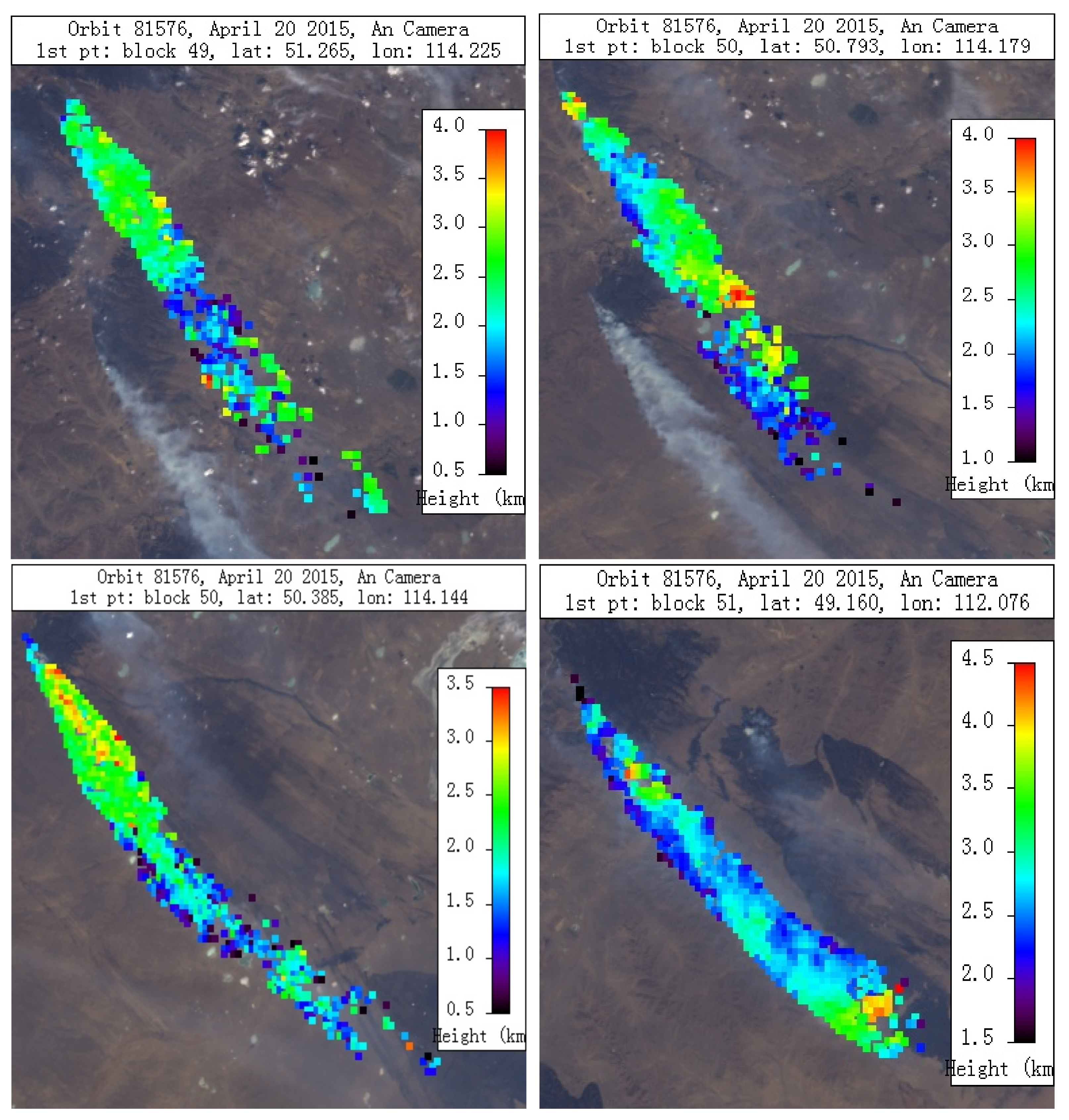
Figure 4.
Burned area from MODIS band 21, and the upper-left corner is the enlarged images of the 3# fire scar.
Figure 4.
Burned area from MODIS band 21, and the upper-left corner is the enlarged images of the 3# fire scar.

Figure 5.
Scatter plots of reflectance of MODIS band 8 vs. Orbiting Carbon Observatory-2 (OCO-2) CO2 concentration in the study region.
Figure 5.
Scatter plots of reflectance of MODIS band 8 vs. Orbiting Carbon Observatory-2 (OCO-2) CO2 concentration in the study region.

Figure 6.
XCO2 values of smoke plumes calculated from MODIS band 8 reflectance.


Table 1.
CO2 emission values and calculated parameters for each fire point by OCO-2.
| Fire Point No. | Smoke Plume Area (103 km2) | Smoke Plume Height (km) | Base XCO2 (ppm) | T (K) | Ba (hPa) | CO2 Emission (103 Mg) |
|---|---|---|---|---|---|---|
| 1# | 2.48 | 2.29 | 399.786 | 281.59 | 906.97 | 156.25 (±4.85) |
| 2# | 2.41 | 2.38 | 122.21 (±4.87) | |||
| 3# | 2.50 | 1.99 | 122.84 (±4.21) | |||
| 4# | 6.48 | 2.61 | 288.70 (±14.33) |
Table 2.
CO2 emission values and calculated parameters for each fire scar using the BBM.
| Fire Point No. | Burned Area (ha) | B × β (Mg/ha) | EF (kg/kg) | CO2 Emission (103 Mg) | Compared with OCO-2 Model |
|---|---|---|---|---|---|
| 1# | 7100 | 38 | 1.489 (0.121) | 401.73 (±32.65) | +157.11% |
| 2# | 2700 | 153.69 (±12.41) | +25.76% | ||
| 3# | 4800 | 271.59 (±22.07) | +121.10% | ||
| 4# | 7500 | 424.37 (±34.49) | +46.99% |
© 2019 by the authors. Licensee MDPI, Basel, Switzerland. This article is an open access article distributed under the terms and conditions of the Creative Commons Attribution (CC BY) license (http://creativecommons.org/licenses/by/4.0/).
Share and Cite
MDPI and ACS Style
Guo, M.; Li, J.; Wen, L.; Huang, S. Estimation of CO2 Emissions from Wildfires Using OCO-2 Data. Atmosphere 2019, 10, 581. https://doi.org/10.3390/atmos10100581
AMA Style
Guo M, Li J, Wen L, Huang S. Estimation of CO2 Emissions from Wildfires Using OCO-2 Data. Atmosphere. 2019; 10(10):581. https://doi.org/10.3390/atmos10100581
Chicago/Turabian StyleGuo, Meng, Jing Li, Lixiang Wen, and Shubo Huang. 2019. "Estimation of CO2 Emissions from Wildfires Using OCO-2 Data" Atmosphere 10, no. 10: 581. https://doi.org/10.3390/atmos10100581
Note that from the first issue of 2016, this journal uses article numbers instead of page numbers. See further details here.