Atmospheric Monitoring of Methane in Beijing Using a Mobile Observatory
by
Wanqi Sun
1, 
Liangchun Deng
2,
Guoming Wu
3,
Lin Wu
4,
Pengfei Han
5,
Yucong Miao
6 and
Bo Yao
1,* 1
Meteorological Observation Centre of China Meteorological Administration, 100081 Beijing, China
2
Center for Environmental Progress, Wuhan 430070, China
3
Hebei Institute of Meteorological Sciences, Shijiazhuang 050021, China
4
State Key Laboratory of Atmospheric Boundary Layer Physics and Atmospheric Chemistry, Institute of Atmospheric Physics, Chinese Academy of Sciences, Beijing 100029, China
5
State Key Laboratory of Numerical Modeling for Atmospheric Sciences and Geophysical Fluid Dynamics, Institute of Atmospheric Physics, Chinese Academy of Sciences, Beijing 100029, China
5
Chinese Academy of Meteorological Sciences, 100081 Beijing, China
*
Author to whom correspondence should be addressed.
Atmosphere 2019, 10(9), 554; https://doi.org/10.3390/atmos10090554
Submission received: 11 August 2019
/
Revised: 7 September 2019
/
Accepted: 12 September 2019
/
Published: 16 September 2019
(This article belongs to the Section Air Quality)
Abstract
:Cities have multiple fugitive emission sources of methane (CH4) and policies adopted by China on replacing coal with natural gas in recent years can cause fine spatial heterogeneities at the range of kilometers within a city and also contribute to the CH4 inventory. In this study, a mobile observatory was used to monitor the real-time CH4 concentrations at fine spatial and temporal resolutions in Beijing, the most important pilot city of energy transition. Results showed that: several point sources, such as a liquefied natural gas (LNG) power plant which has not been included in the Chinese national greenhouse gas inventory yet, can be identified; the ratio “fingerprints” (CH4:CO2) for an LNG carrier, LNG filling station, and LNG power plant show a shape of “L”; for city observations, the distribution of CH4 concentration, in the range of 1940–2370 ppbv, had small variations while that in the rural area had a much higher concentration gradient; significant correlations between CO2 and CH4 concentrations were found in the rural area but in the urban area there were no such significant correlations; a shape of “L” of CH4:CO2 ratios is obtained in the urban area in wintertime and it is assigned to fugitive emissions from LNG sources. This mobile measurement methodology is capable of monitoring point and non-point CH4 sources in Beijing and the observation results could improve the CH4 inventory and inform relevant policy-making on emission reduction in China.
1. Introduction
Methane (CH4) contributes ~17% of the radiative forcing by the long-lived greenhouse gases (GHG) [1], with global warming potential (GWP) more than 25 times greater than that of CO2 at a 100-yr time horizon [2]. Its mean annual increase rate witnessed no growth during 1999–2006 but has been increasing again since 2007 [1,3]. Increased emission from anthropogenic sources at mid-latitudes of the northern hemisphere has been considered as one possible main contributor of the recent increase [1,3], while some estimates indicated that China is the world’s largest anthropogenic emitter of CH4 [4]. Therefore, it is essential to quantify the anthropogenic sources of CH4 emissions in China and further evaluate their contributions. Cities, especially in Northern China, are generally important anthropogenic sources of CH4 [5]. In megacities of China, the total natural gas (NG) consumption increased about seven times over the last 16 years (2000–2016) [6] with policies adopting the replacement of coal with gas launched by the Chinese government [5,7,8]. The increasing proportion of NG utilization together with increasing energy demands might lead to complex changes in the spatial and temporal pattern of atmospheric CH4 concentrations, as well as the emission inventory [5,9,10]. To better understand the quantitative information, field monitoring at fine spatial and temporal scales in cities is necessary.
Presently, there are several monitoring tools for CH4 emissions, such as satellite remote sensing [11,12,13,14], ground station observation [15,16], mobile observation by aircraft [14,17,18,19] or by car [20,21,22,23,24]. Satellite remote sensing technology is applied for observations mainly at the global or continental scales. Ground-based observation using stationary measurement towers is generally adopted by World Meteorological Organization (WMO) Global Atmosphere Watch (GAW) surface-based global or regional background stations [15,16]. It boasts higher precision than satellite remote sensing, but the high costs of establishment and maintenance have limited the development of an extensive network. Thus, it would be quite difficult to implement such a technology to resolve spatial heterogeneities in a city scale and to track moving sources [25]. In addition, aerial surveys can also offer intensive measurements for the distribution and quantification of sources and sinks of CH4 at city, regional or terrestrial scales [19,26,27,28,29,30], but that kind of measurement is often restricted due to the strict air traffic control in China. A ground-based mobile observatory has more flexibility of use than aircraft, and it has been adopted by several CH4 research projects [9,20,21,22,24,25,31,32]. The vehicles used include public transit, for example, light-rail platform [25], and ordinary cars [22,31]. Moreover, surveyed fugitive emission covered an extensive range of sources, including combustions [31,33], pipeline [21] and gas infrastructure leaks [22,23], NG developments [20], landfills [22], and oil producing regions [33]. Meanwhile, observed areas are mainly the urban areas [22,23,31,34]. Thus, the mobile ground-based observatory has been tested sufficiently with a wide range of applications to measure point and non-point sources of CH4. However, although a qualitative measurement in Beijing for the purpose to verify the performances of their instrument was conducted [34], comprehensive CH4 concentration of the entire city and the characteristic of different types of sources in Northern China by a mobile observatory has not been reported.
The goal of this work was to set up a ground-based mobile observatory and to measure the concentration of atmospheric CH4 in Beijing with high precision, which has a population of ~19.6 million and has the largest demand of winter-heating services among cities in China [35]. Beijing is also suffering heavy air pollution [36,37] and taking efforts to replace coal by NG to improve air quality. Nearly all of the coal-fired boilers, including power generating boilers, have been changed into gas ones or air conditioners up to 2017. Studying the concentration of atmospheric CH4 in Beijing could tremendously inform the CH4 inventory and relevant policy-making on GHG emission reduction in China.
2. Experimental Design
2.1. Mobile Observatory for CH4
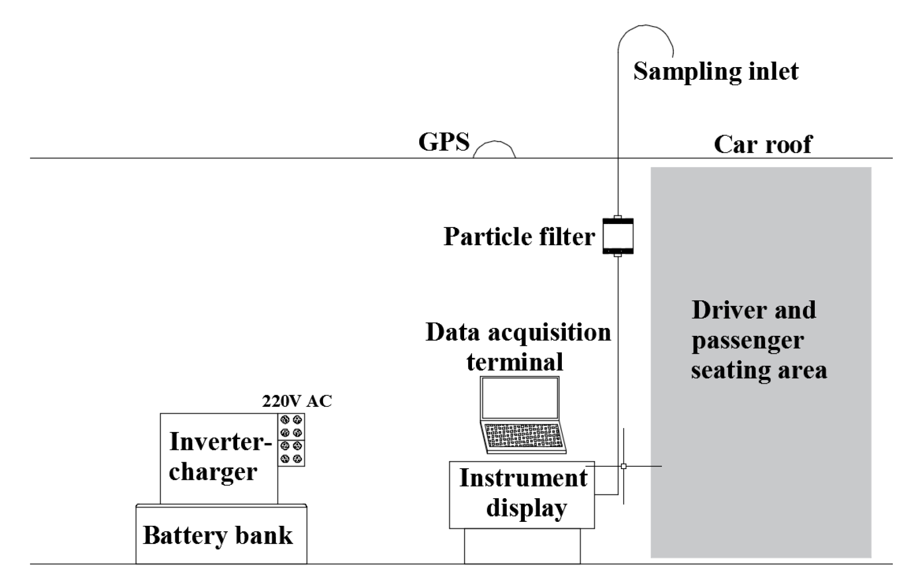
The structure of the mobile observatory (MO) used in this work is illustrated in Figure 1. A multi-purpose vehicle (MPV, A800, Chang’ an Automobile Group, Chongqing, China) with a sunroof was selected as the mobile platform. The components of this MO included electrical power, a high precision CH4 analyzer, a global positioning system (GPS) receiver and a data acquisition device. The electric power was provided as 220V AC via an inverter-charger which was a 12 V, 3000 W, pure sine-wave inverter that served a number of different functions (HS-3KRH, Foshan Baykee New Energy Technology Incorporated Company, Foshan, China). The inverter-charger provided 220V AC from a 12V DC supply associated with a battery bank. The battery bank consisted of two lithium ion batteries (300 Ah each), wired in parallel and connected to the inverter-charger. The high precision CH4 analyzed was based on a cavity ring-down spectrometer (CRDS) technique (G1301 and 2401, Picarro, Santa Clara, CA, USA). The measurement precision of G1301 was better than 0.7 ppbv for CH4 (5 min average) and that of G2401 was 0.5 ppbv. Ambient air was collected through tubing (1/4” OD, ~2 m long, Synflex-1300, Aurora, CO, USA) from the inlet ~0.35 m over the sunroof, or ~2.2 m above the road surface. Particles were removed by a filter (0.2 μm, Ploycap 75, 0.2 PTFE, Buckinghamshire, UK) before it was assessed by the CRDS analyzer, with a measurement interval of approximately 3 s (G1302) and 1.2 s (G2401). Considering that the speed of the car was 40 to 80 kilometers per hour, the spatial resolution of this observation method was approximately 10–20 m. Additional technical information for the CRDS analyzer can be found in previous studies [38]. Before and after each observation mission, the CRDS analyzer was calibrated by standard gases which traced to WMO X2004A scale for CH4, X2007 scale for CO2, and WMO-2014A scale for CO to correct the drift of the analyzer. The geographic location of the vehicle platform was obtained by a GPS receiver (BS-70DU, Shenzhen Beitian Communication Co., Ltd., Shenzhen, China), mounted inside the car with an accuracy of approximately 2 m. Data from the CRDS analyzer and GPS receiver were recorded each 1.2 s by a laptop computer (Tsinghua Tongfang Co., Ltd., Beiing, China, T45PRO-Gcc-21053). The data system time was synchronized with the GPS system time so that the data file and GPS files could be merged in real time.
2.2. Measurement Routes and Strategies
Table 1 shows the measurement strategies in Beijing. Firstly, five kinds of point sources, including a liquefied natural gas (LNG) carrier, an LNG station, a residential area, an LNG power plant and a refuse landfill, were surveyed to elucidate their concentration characteristics and ratio “fingerprints” (CH4:CO2). Secondly, the city was surveyed to determine their overall concentration characteristics and to identify the major CH4 emitters. Outward from the city center of Beijing, there are five ring roads that circle the city, the 2nd (32.7 km), the 3rd (48 km), the 4th (64 km), the 5th (99 km), and the 6th (192 km) ring road. The 2nd–4th, 5th, and 6th ring roads are located in the urban, suburban and rural area of the city, respectively. In this study, observations at the 2nd–4th ring roads represented the urban area and the 6th ring road represented the rural area. Climatically, there are four distinctive seasons (spring, summer, autumn, and winter) in Beijing. Heating is necessary over the winter months (annually often from mid-November to mid-March), but not at other times of the year. In this study, “wintertime” and “non-wintertime” were used to characterize the application of heating services. When conducting the monitoring, since the battery used in the measurement can only supply power for ~5 h to the G1302 in the non-wintertime, the 2nd–4th and 6th ring roads were surveyed on different days and each for three times. For G2401 used in the wintertime, the battery was sufficient for surveys of all the ring roads (2nd–6th) on a single day. All the measurements were conducted during the daytime. The weather conditions and average wind speed, which were directly associated with the diffusion conditions, were also captured from observation, as listed in Table 1.
2.3. Data Analysis
According to the observation log, invalid data were identified and flagged. The concentration data of CH4 and CO2 were calibrated by standard gases, as was the time data for the delayed response of the sampling system for 55 s. Finally, the CH4 concentration data, along with the meteorological data obtained from the meteorological stations adjacent to the observed areas, were combined with GPS data to generate spatial information data using the Arc GIS software.
To understand the correlation of CH4 and CO2 for fugitive emissions and city-scale emissions of Beijing, the minimum concentration value was subtracted from each survey as background to create a dataset of differences, or “enhanced” (e) concentrations which means the observed concentration minus background values and represent the enhancement for a gas species (eCO2, eCH4). The data processing method refers to what Hurry et al. used in the observation activity in oil producing regions in North America [33].
3. Result and Discussion
3.1. Point Source Observation in Beijing
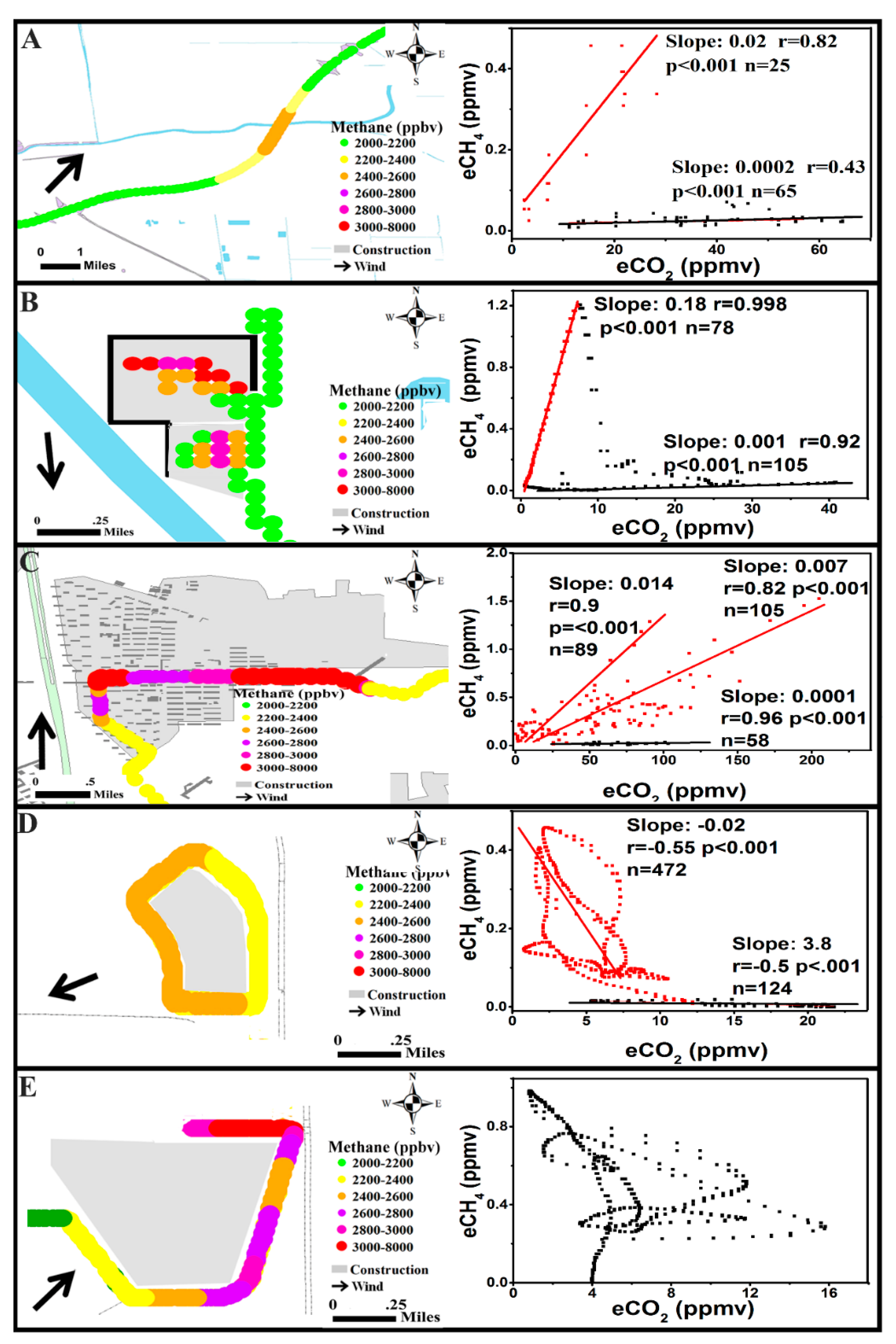
Figure 2 shows map transections of CH4 and ratio “fingerprints” (CH4:CO2) of five point sources in Beijing. Figure 2A shows the screening result of an LNG carrier. A hotspot was captured with peak concentration up to 2524 ppbv. Its CH4:CO2 ratios show a shape of “L” of high CH4 values versus low CO2 values (slope = 0.02, r = 0.82, p < 0.001), and high CO2 concentrations versus low CH4 concentrations (slope = 0.0002, r = 0.43, p < 0.001). This is similar to the survey result of gas regulator stations [22]. The slope 0.0002 could be used to deduce that it mainly originated from the vehicle exhaust [33] and the slope 0.02 was associated with the release of CH4 from storage facilities in the carrier [22].
Figure 2B presents the CH4 map transection of an LNG filling station in the suburban area. One hotspot with maximum concentration 4777 ppbv appeared at the site adjacent to the LNG storage facility in the station while another with 2799 ppbv on the side of a working gas gun. Its CH4:CO2 ratios also shows a shape of “L” (CH4:CO2 = 0.18 and 0.001). The slope 0.18 is higher than 0.02 shown in Figure 2A by one order of magnitude which describes a different type of source profile, although it may be specific to the time and location.
Figure 2C shows the CH4 map transection of a residential area at cooking time using gas for cooking. One hotspot with peak concentration 3436 ppbv emerged in the residential area while another one with maximum concentration 3448 ppbv on the side of it. The CH4:CO2 ratios of the two hotspots are 0.014 (r = 0.9, p < 0.001) and 0.007 (r = 0.82, p < 0.001). They may associate with the leakage of CH4 pipelines or combustion devices [22,33].
Figure 2D shows the survey result of an LNG power plant. The MO circled the plant for three times and the concentration distributions obtained were similar, namely, concentrations being low in the upwind side and high in the downwind side. The CH4:CO2 ratios also reflected a characteristic “L” pattern (–0.02, r = –0.55, p < 0.001 and 3.8, r = 0.5, p < 0.001), but the “L” was different from Figure 2A,B and one of the slopes was negative. This may have been associated with the relationship between the CH4 supply and the combustion efficiency of the boiler.
Figure 2E shows the survey result of a refuse landfill. High concentration was in the downwind east and northeast of site. The wind distribution and the existence of the CH4 disposing plant located in the east of the landfill have contributed to such concentration distribution. The characteristic of CH4:CO2 ratios were complex, which were different to the other four sources mentioned above. The complexity may have generated from the multiple CH4 sources in the landfill, such as the landfill itself with the biological processes, the landfill leachate, the collecting pipelines of CH4, the burning of the collected CH4 in the disposing plant, and the garbage trucks.
In short, the MO had enough temporal and spatial resolution to identify the typical point sources of CH4 in both urban and rural areas in Beijing. The ratio “fingerprints” for the point sources using LNG all showed a characteristic “L” pattern, which was useful to distinguish different CH4 sources in the city.
3.2. City Observation in the Non-Wintertime Period
Figure 3 shows results of the urban (the 2nd–4th ring roads) and rural area (the 6th ring road) of Beijing in non-wintertime. The boxplot method was used to show the distribution characteristics of the observed CH4 concentration data, whose statistical results are shown in Table 2. It includes the values of minimum, maximum, median, upper quartile (Q1), lower quartile (Q2), inter-quartile range (IQR), and maximum outlier and number of valid data for each measurement. Note that the outliers are the values outside of the box body (less than Q1 − 1.5 × IQR or higher than Q3 + 1.5 × IQR).
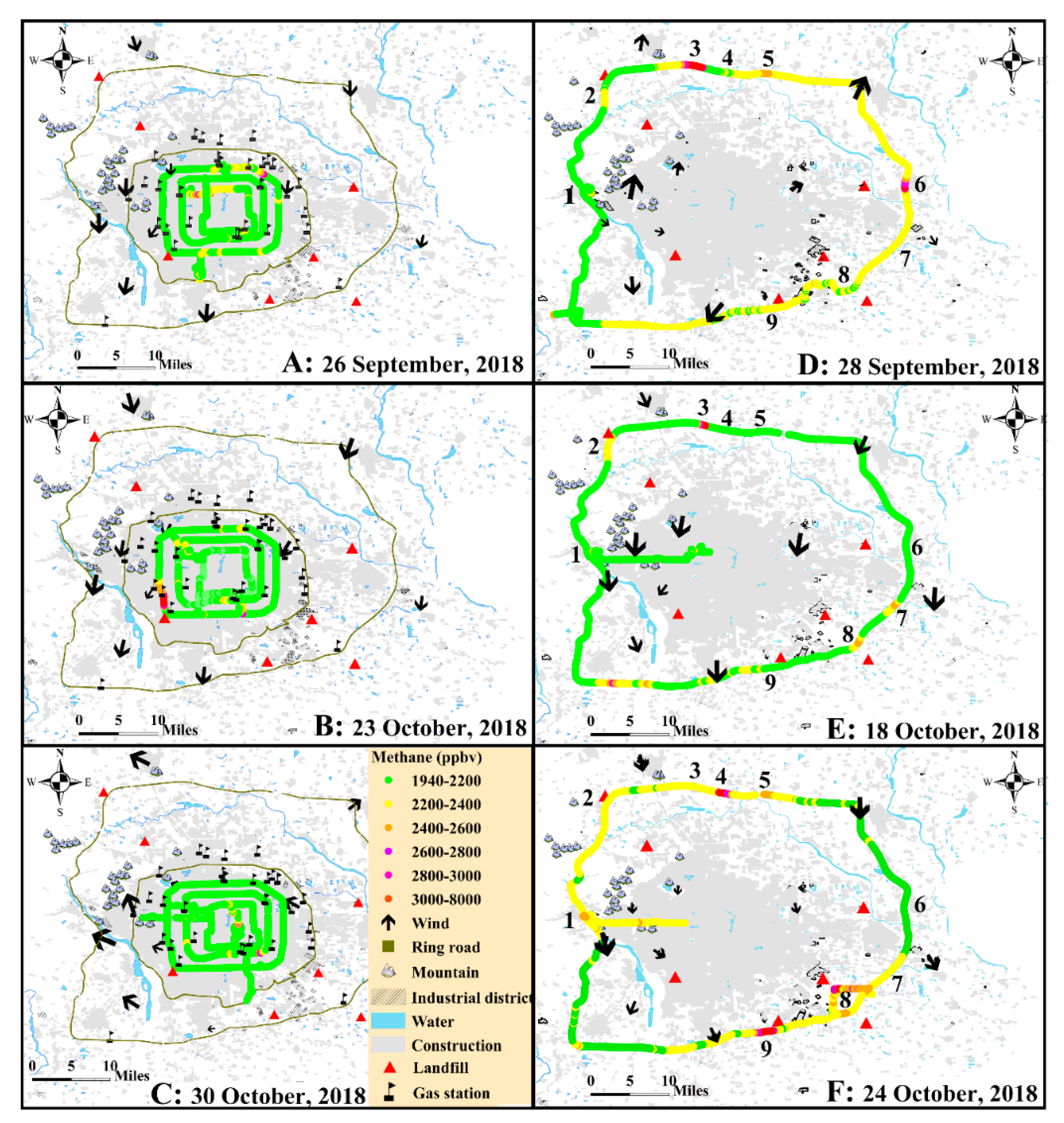
Figure 3A–C present the CH4 map transections of the urban area on 26 September, 23 October, and 30 October, 2018, respectively. Generally, the concentrations for the three survey days mainly ranged from 1940 to 2370 ppbv, which are obviously higher than that reported in 2000 (1870–2000 ppbv) [39] in the urban area and similar to that measured during 2009–2014 by WMO/GAW Shangdianzi regional background station (1850–2400 ppbv) which is 100 km away from the urban area16. The concentration gradient was relatively small, implying that the urban area might be treated as a typical non-point source of CH4. However, some hotspots, whose concentration were higher than 2800 ppbv, were observed during all surveys with different locations, indicating that some intermittent or mobile fugitive leaks may exist, for example, underground transmission, distribution pipelines or usages by the residents [31].
Figure 3D–F show the CH4 map transections of the rural area on 28 September, 18 October, and 24 October, 2018, respectively. The concentrations for the three surveys mainly distributed between 2016–2515 ppbv, which were notably higher than those of the urban area mentioned above. The dispersion of these data was also higher than those of the urban area through comparing the inter-quartile range (IQRs). There were obviously concentration gradients up to several hundred ppbv, in Figure 3D,F, but not in Figure 3E. Higher concentrations were observed both in areas upwind and downwind of urban Beijing, which revealed that the local emission might be the main impact factor rather than the CH4 emission from urban area. Moreover, eight notable hotspots were captured. The concentrations of hotspot 1 (2400–2600 ppbv) were just slightly higher than its surroundings (2000–2400 ppbv). It was identified to be a LNG power plant, which was a source not included by the methane inventory of China [5], through the method mentioned in Section 3.1 and the field investigation. The hotspot 2 (2200–2400 ppbv) could be recognized in all three surveys, mainly due to the nearby landfill. Hotspot 3 emerged with the maximum concentration 7657 ppbv in Figure 3D,E. It might have been a stationary fugitive source, such as NG pipeline leak, which existed before 28 September, 2018 and was presumably remediated between 18 October, and 24 October, 2018. Hotspots 4–9 emerged randomly in the three figures. Hotspot 7 was identified as the LNG carrier (Figure 2A) and hotspot 8 was a residential area (Figure 2C). But the sources for hotspots 4–6 and 9 were not identified. According to their characteristic, they were speculated to be associated with mobile gas carriers or intermittent sources, such as leakages of underground transmission and distribution pipelines.
3.3. City Observation in the Wintertime Period
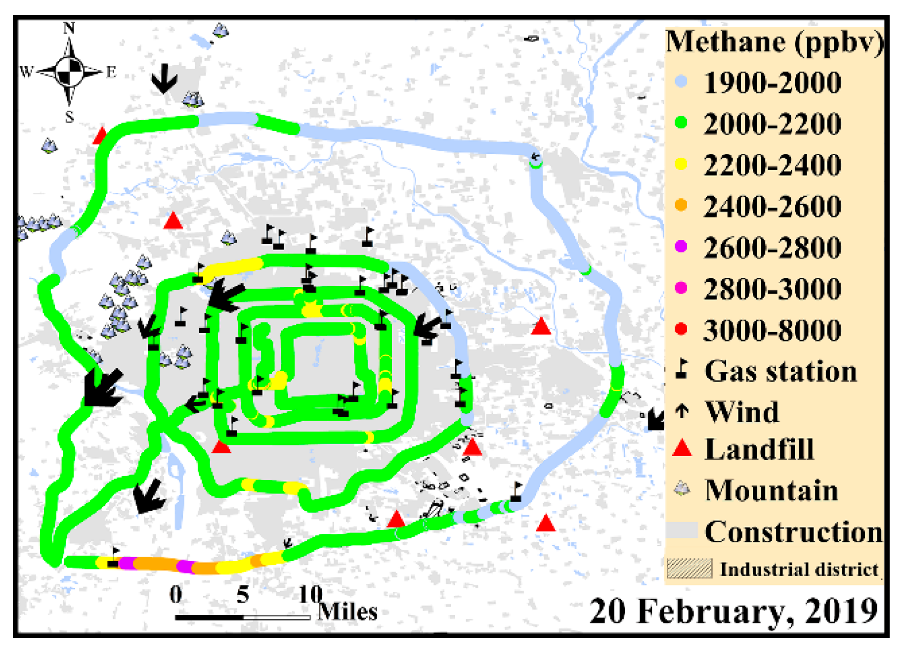
Figure 4 shows the result of survey on 20 February, 2019 which was in the wintertime. The statistical results of the urban and rural area are presented in Table 2. The CH4 concentrations for the urban area (the 2nd–4th ring roads) were mainly in the range of 2059–2248 ppbv and it was similar to that obtained in the non-wintertime. The CH4 concentrations for the rural area (the 6th ring road) were mainly between 1953–2276 ppbv, lower than that obtained in the non-wintertime. There was a remarkable concentration gradient. Higher concentrations were found in the southwest area and lower in the northeast part. Meanwhile, concentrations were much higher in the downwind area than the upwind area, similar to the observation result in urban area of eastern Germany [23]. Several hotspots were observed and their identifications were similar to that discussed in Section 3.2.
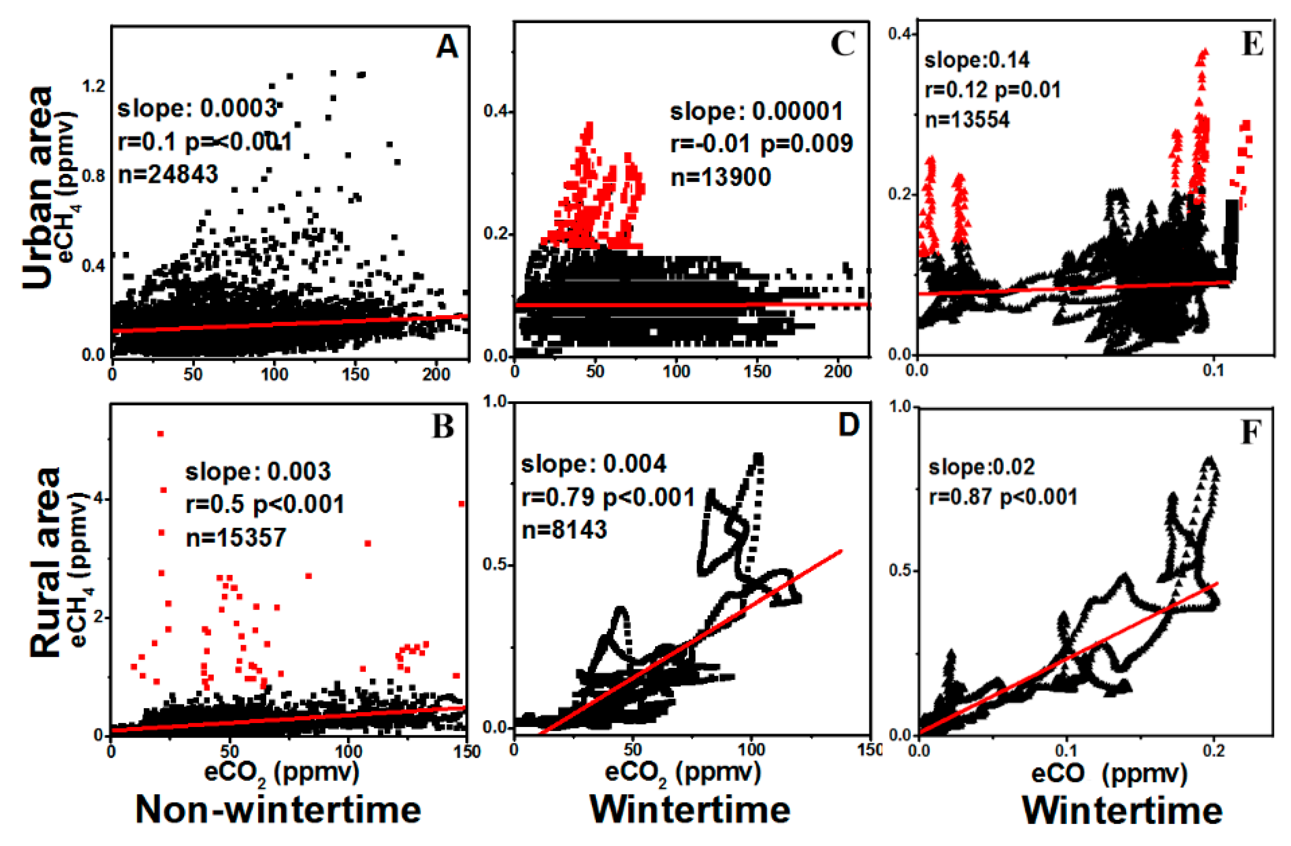
Figure 5A–D shows the relationship between the CH4 and CO2 concentrations measured in non-winter and wintertime. Regression analysis was used to determine the CH4/CO2 ratio. The regression coefficients (r) in Figure 5A,C were both quite small, demonstrating that the correlation of CH4 and CO2 enhanced concentrations in the urban of Beijing was quite weak, in contrast to the significant correlation in research conducted in Nanjing [40]. Our study provided high spatial resolution data of CH4 and CO2, while a fixed sensor is used by the study in Nanjing on a higher floor of a building, which might explain that stronger correlations between CH4 and CO2 were observed since they were sensitive to more mixed air within the footprint of their sensor. In Figure 5C, the red outliers are with high CH4 concentrations but small or even negative CO2 elevation makes the whole figure a shape of “L”. This “L” pattern was similar to that of the LNG point sources, such as the passing-by LNG carrier, the LNG filling station, or the LNG power plant (see Figure 2A,B,D, respectively), which indicated that LNG sources might have contributed to CH4 enhancement in this survey. The enhanced CH4 concentrations had significant correlation (p < 0.001) with CO2 enhancements in the rural area with regression coefficient (r) of 0.5 and 0.79 in Figure 5B,D, respectively. The regression slope (CH4:CO2) for the rural area was 0.003 in non-wintertime and 0.004 in wintertime. The slope 0.004 was comparable to that obtained in Boulder [41] and Indianapolis [30], USA. It should be noted that different methodologies were applied in these studies and the differences introduced by methodologies were not considered.
CO concentrations were also observed in wintertime. Figure 5E,F shows the relationship between the CH4 and CO concentrations in wintertime. In Figure 5E, similar to that of CH4/CO2 in Figure 5A,C, the regression coefficients (r) was quite small, revealing that the correlation of CH4 and CO enhanced concentrations in the urban of Beijing was quite weak. Meanwhile, obvious CH4 fugitive emissions could be seen (red dots). This revealed that the CH4 sources were complicated in the urban area. Shown in Figure 5F, the enhanced CH4 concentrations had significant correlation (p < 0.001) with CO enhancements in the rural area with a regression coefficient (r) of 0.87, which was similar to the significant correlation of CH4 and CO2 shown in Figure 5B,D. This indicated the high CO2/CH4/CO concentrations in winter might have been influenced by combustion or by well mixed anthropogenic emissions from other sources in Beijing city.
4. Conclusions
A mobile observatory was applied to real-time monitor the CH4 concentration of point and non-point (city) sources in Beijing. The results indicated that this mobile measurement methodology has enough temporal and spatial resolution to identify typical CH4 sources in Beijing. The ratio “fingerprints” (CH4:CO2) for the LNG carrier, LNG filling station, and LNG power plant showed a characteristic “L” pattern which may reveal typical point sources with LNG leakage. For city observations in non-wintertime, the CH4 concentrations were in the range of 1940–2370 ppbv and those in the rural area were 2016–2515 ppbv. Several fugitive point sources, including LNG power plant and landfill, were successfully identified in the rural measurement. As for city observation in wintertime, the CH4 concentrations were mainly in the range of 2059–2248 ppbv, which was comparable to that in the non-wintertime observations, while concentrations in the rural area (1953–2276 ppbv) also had an obvious concentration gradient. According to the correlation analysis, the CH4 and CO2 enhanced concentration showed significant correlation in the rural area, but not in the urban area. A shape of “L” was obtained and it suggested fugitive emissions from the NG sources in wintertime. Further attempts of CH4 emission study by inverse modeling on a city scale would help understanding the observed signals. Similar studies report the quantification of CH4 emission by mobile measurement platform such as airplanes [42,43].
Supplementary Materials
The following are available online at https://www.mdpi.com/2073-4433/10/9/554/s1.
Author Contributions
Conceptualization, B.Y.; Methodology, B.Y. and W.-Q.S.; Software, W.-Q.S. and B.Y.; Validation, B.Y. and W.-Q.S.; Formal Analysis, W.-Q.S. and B.Y.; Investigation, W.-Q.S.; Resources, B.Y.; Data Curation, W.-Q.S.; Writing-Original Draft Preparation, W.-Q.S.; Writing-Review & Editing, L.-C.D., B.Y., L.W., P.-F.H., and Y.-C.M.; Visualization, W.-Q.S. and G.-M.W.; Supervision, B.Y.; Project Administration, W.-Q.S.; Funding Acquisition, B.Y.
Funding
This work was supported by the National Key R&D Program of China (2017YFB0504000) and the National Natural Science Foundation of China (NO. 41705134 and 41575114).
Acknowledgments
We thank National Oceanic and Atmospheric Administration (NOAA)/Earth System Research Laboratory (ESRL) for providing tertiary standard gases. We also thank Hongyang Wang for calibrating the instruments used in the study.
Conflicts of Interest
The authors declare no conflict of interest. The funders had no role in the design of the study; in the collection, analyses, or interpretation of data; in the writing of the manuscript, and in the decision to publish the results.
References
- WMO. Greenhouse Gas Bulletin: The State of Greenhouse Gases in the Atmosphere Based on Global Observations through 2017; WMO: Geneva, Switzerland, 2017. [Google Scholar]
- Solomon, S.; Qin, D.; Manning, M.; Averyt, K.; Marquis, M. Climate Change 2007—The Physical Science Basis: Working Group I Contribution to the Fourth Assessment Report of the IPCC; Cambridge University Press: Cambridge, UK, 2007; Volume 4. [Google Scholar]
- Fletcher, S.E.M.; Schaefer, H. Rising methane: A new climate challenge. Science 2019, 364, 932–933. [Google Scholar] [CrossRef] [PubMed]
- Korsbakken, J.I.; Peters, G.P.; Andrew, R.M. Uncertainties around reductions in China’s coal use and CO2 emissions. Nat. Clim. Chang. 2016, 6, 687–691. [Google Scholar] [CrossRef]
- Cai, B.f.; Zhang, J.J.; Dong, H.J.; Yao, B. The Illustrated Handbook of Greenhouse Gas Emissions from Chinese Cities 2015; China Environmental Science Press: Beijing, China, 2019. [Google Scholar]
- MOHURD—Ministry of Housing and Urban-Rural Development of the People’s Republic of China. China Urban Construction Statistical Yearbook 2013–2017; MOHURD: Beijing, China, 2018. [Google Scholar]
- Cui, Y.; Zhang, W.; Wang, C.; Streets, D.G.; Xu, Y.; Du, M.; Lin, J. Spatiotemporal dynamics of CO2 emissions from central heating supply in the North China Plain over 2012–2016 due to natural gas usage. Appl. Energy 2019, 241, 245–256. [Google Scholar] [CrossRef]
- Shen, G.; Ru, M.; Du, W.; Zhu, X.; Zhong, Q.; Chen, Y.; Shen, H.; Yun, X.; Meng, W.; Liu, J. Impacts of air pollutants from rural Chinese households under the rapid residential energy transition. Nat. Commun. 2019, 10, 1–8. [Google Scholar] [CrossRef] [PubMed] [Green Version]
- McKain, K.; Down, A.; Raciti, S.M.; Budney, J.; Hutyra, L.R.; Floerchinger, C.; Herndon, S.C.; Nehrkorn, T.; Zahniser, M.S.; Jackson, R.B. Methane emissions from natural gas infrastructure and use in the urban region of Boston, Massachusetts. Proc. Natl. Acad. Sci. USA 2015, 112, 1941–1946. [Google Scholar] [CrossRef] [PubMed] [Green Version]
- Alvarez, R.A.; Zavala-Araiza, D.; Lyon, D.R.; Allen, D.T.; Barkley, Z.R.; Brandt, A.R.; Davis, K.J.; Herndon, S.C.; Jacob, D.J.; Karion, A. Assessment of methane emissions from the US oil and gas supply chain. Science 2018, 361, 186–188. [Google Scholar] [PubMed]
- Butz, A.; Guerlet, S.; Hasekamp, O.; Schepers, D.; Galli, A.; Aben, I.; Frankenberg, C.; Hartmann, J.M.; Tran, H.; Kuze, A. Toward accurate CO2 and CH4 observations from GOSAT. Geophys. Res. Lett. 2011, 38, 130–137. [Google Scholar] [CrossRef]
- Buchwitz, M.; Reuter, M.; Bovensmann, H.; Pillai, D.; Heymann, J.; Schneising, O.; Rozanov, V.; Krings, T.; Burrows, J.; Boesch, H. Carbon Monitoring Satellite (CarbonSat): Assessment of atmospheric CO2 and CH4 retrieval errors by error parameterization. Atmos. Meas. Tech. 2013, 6, 3477–3500. [Google Scholar] [CrossRef]
- Saitoh, N.; Touno, M.; Hayashida, S.; Imasu, R.; Shiomi, K.; Yokota, T.; Yoshida, Y.; Machida, T.; Matsueda, H.; Sawa, Y. Comparisons between XCH4 from GOSAT shortwave and thermal infrared spectra and aircraft CH4 measurements over Guam. SOLA 2012, 8, 145–149. [Google Scholar] [CrossRef]
- Xiong, X.; Barnet, C.D.; Zhuang, Q.; Machida, T.; Sweeney, C.; Patra, P.K. Mid-upper tropospheric methane in the high Northern Hemisphere: Spaceborne observations by AIRS, aircraft measurements, and model simulations. J. Geophys. Res. Atmos. 2010, 115, 1–15. [Google Scholar] [CrossRef]
- Fang, S.X.; Zhou, L.X.; Masarie, K.A.; Xu, L.; Rella, C.W. Study of atmospheric CH4 mole fractions at three WMO/GAW stations in China. J. Geophys. Res. Atmos. 2013, 118, 4874–4886. [Google Scholar] [CrossRef]
- Fang, S.-X.; Tans, P.P.; Dong, F.; Zhou, H.; Luan, T. Characteristics of atmospheric CO2 and CH4 at the Shangdianzi regional background station in China. Atmos. Environ. 2016, 131, 1–8. [Google Scholar] [CrossRef]
- Nakazawa, T.; Sugawara, S.; Inoue, G.; Machida, T.; Makshyutov, S.; Mukai, H. Aircraft measurements of the concentrations of CO2, CH4, N2O, and CO and the carbon and oxygen isotopic ratios of CO2 in the troposphere over Russia. J. Geophys. Res. Atmos. 1997, 102, 3843–3859. [Google Scholar] [CrossRef]
- Gerilowski, K.; Tretner, A.; Krings, T.; Buchwitz, M.; Bertagnolio, P.P.; Belemezov, F.; Erzinger, J.; Burrows, J.P.; Bovensmann, H. MAMAP—A new spectrometer system for column-averaged methane and carbon dioxide observations from aircraft: Instrument description and performance analysis. Atmos. Meas. Tech. 2011, 4, 215–243. [Google Scholar] [CrossRef]
- Karion, A.; Sweeney, C.; Wolter, S.; Newberger, T.; Chen, H.; Andrews, A.; Kofler, J.; Neff, D.; Tans, P. Long-term greenhouse gas measurements from aircraft. Atmos. Meas. Tech. 2013, 6, 511–526. [Google Scholar] [CrossRef] [Green Version]
- Atherton, E.; Risk, D.; Fougère, C.; Lavoie, M.; Marshall, A.; Werring, J.; Williams, J.P.; Minions, C. Mobile measurement of methane emissions from natural gas developments in northeastern British Columbia, Canada. Atmos. Chem. Phys. 2017, 17, 12405–12420. [Google Scholar] [CrossRef] [Green Version]
- LeIfer, I.; Melton, C.; Manish, G.; Leen, B. Mobile Monitoring of Methane Leakage; Gases and Instrumentation, Gases and Instrumentation International: Wellesley Hills, MA, USA, 2014. [Google Scholar]
- Lamb, B.K.; McManus, J.B.; Shorter, J.H.; Kolb, C.E.; Mosher, B.; Harriss, R.C.; Allwine, E.; Blaha, D.; Howard, T.; Guenther, A. Development of atmospheric tracer methods to measure methane emissions from natural gas facilities and urban areas. Environ. Sci. Technol. 1995, 29, 1468–1479. [Google Scholar] [CrossRef] [PubMed]
- Shorter, J.H.; Mcmanus, J.B.; Kolb, C.E.; Allwine, E.J.; Lamb, B.K.; Mosher, B.W.; Harriss, R.C.; Partchatka, U.; Fischer, H.; Harris, G.W. Methane emission measurements in urban areas in eastern Germany. J. Atmos. Chem. 1996, 24, 121–140. [Google Scholar] [CrossRef]
- Lamb, B.K.; Cambaliza, M.O.; Davis, K.J.; Edburg, S.L.; Ferrara, T.W.; Floerchinger, C.; Heimburger, A.M.; Herndon, S.; Lauvaux, T.; Lavoie, T. Direct and indirect measurements and modeling of methane emissions in Indianapolis, Indiana. Environ. Sci. Technol. 2016, 50, 8910–8917. [Google Scholar] [CrossRef] [PubMed]
- Mitchell, L.E.; Crosman, E.T.; Jacques, A.A.; Fasoli, B.; Leclair-Marzolf, L.; Horel, J.; Bowling, D.R.; Ehleringer, J.R.; Lin, J.C. Monitoring of greenhouse gases and pollutants across an urban area using a light-rail public transit platform. Atmos. Environ. 2018, 187, 9–23. [Google Scholar] [CrossRef]
- Choi, Y.; Vay, S.A.; Vadrevu, K.P.; Soja, A.J.; Woo, J.H.; Nolf, S.R.; Sachse, G.W.; Diskin, G.S.; Blake, D.R.; Blake, N.J. Characteristics of the atmospheric CO2 signal as observed over the conterminous United States during INTEX-NA. J. Geophys. Res. Atmos. 2008, 113, 1–16. [Google Scholar] [CrossRef]
- Brenninkmeijer, C.; Crutzen, P.; Boumard, F.; Dauer, T.; Dix, B.; Ebinghaus, R.; Filippi, D.; Fischer, H.; Franke, H.; Frieβ, U.; et al. Civil aircraft for the regular investigation of the atmosphere based on an instrumented container: The new CARIBIC system. Atmos. Chem. Phys. 2007, 7, 4953–4976. [Google Scholar] [CrossRef]
- Kort, E.A.; Eluszkiewicz, J.; Stephens, B.B.; Miller, J.B.; Gerbig, C.; Nehrkorn, T.; Daube, B.C.; Kaplan, J.O.; Houweling, S.; Wofsy, S.C. Emissions of CH4 and N2O over the United States and Canada based on a receptor-oriented modeling framework and COBRA-NA atmospheric observations. Geophys. Res. Lett. 2008, 35, 1–5. [Google Scholar] [CrossRef]
- Cambaliza, M.; Shepson, P.; Bogner, J.; Caulton, D.; Stirm, B.; Sweeney, C.; Montzka, S.; Gurney, K.; Spokas, K.; Salmon, O. Quantification and source apportionment of the methane emission flux from the city of Indianapolis. Elem. Sci. Anth. 2015, 3, 1–18. [Google Scholar] [CrossRef]
- Mays, K.L.; Shepson, P.B.; Stirm, B.H.; Karion, A.; Sweeney, C.; Gurney, K.R. Aircraft-based measurements of the carbon footprint of Indianapolis. Environ. Sci. Technol. 2009, 43, 7816–7823. [Google Scholar] [CrossRef]
- Bush, S.; Hopkins, F.; Randerson, J.; Lai, C.; Ehleringer, J. Design and application of a mobile ground-based observatory for continuous measurements of atmospheric trace gas and criteria pollutant species. Atmos. Meas. Tech. 2015, 8, 33–63. [Google Scholar] [CrossRef]
- Yacovitch, T.I.; Herndon, S.C.; Pétron, G.; Kofler, J.; Lyon, D.; Zahniser, M.S.; Kolb, C.E. Mobile laboratory observations of methane emissions in the barnett shale region. Environ. Sci. Technol. 2015, 49, 7889–7895. [Google Scholar] [CrossRef]
- Hurry, J.; Risk, D.; Lavoie, M.; Brooks, B.-G.; Phillips, C.L.; Göckede, M. Atmospheric monitoring and detection of fugitive emissions for Enhanced Oil Recovery. Int. J. Greenh. Gas Control 2016, 45, 1–8. [Google Scholar] [CrossRef]
- Tao, L.; Sun, K.; Miller, D.J.; Pan, D.; Golston, L.M.; Zondlo, M.A. Low-power, open-path mobile sensing platform for high-resolution measurements of greenhouse gases and air pollutants. Appl. Phys. B 2015, 119, 153–164. [Google Scholar] [CrossRef]
- PCOSC. Tabulation on the 2010 Population Census of the People’s Republic of China; China Statistics Press: Beijing, China, 2010. [Google Scholar]
- Miao, Y.; Liu, S. Linkages between aerosol pollution and planetary boundary layer structure in China. Sci. Total Environ. 2019, 650, 288–296. [Google Scholar] [CrossRef]
- Miao, Y.; Liu, S.; Guo, J.; Huang, S.; Yan, Y.; Lou, M. Unraveling the relationships between boundary layer height and PM2.5 pollution in China based on four-year radiosonde measurements. Environ. Pollut. 2018, 243, 1186–1195. [Google Scholar] [CrossRef] [PubMed]
- Crosson, E. A cavity ring-down analyzer for measuring atmospheric levels of methane, carbon dioxide, and water vapor. Appl. Phys. B 2008, 92, 403–408. [Google Scholar] [CrossRef]
- Wang, Y.S.; Zhou, L.; Wang, M.X.; Zheng, X.H. Trends of atmospheric methane in Beijing. Chemosphere Glob. Chang. Sci. 2001, 3, 65–71. [Google Scholar] [CrossRef]
- Shen, S.; Yang, D.; Xiao, W.; Liu, S.; Lee, X. Constraining anthropogenic CH4 emissions in Nanjing and the Yangtze River Delta, China, using atmospheric CO2 and CH4 mixing ratios. Adv. Atmos. Sci. 2014, 31, 1343–1352. [Google Scholar] [CrossRef]
- Conway, T.; Steele, L. Carbon dioxide and methane in the Arctic atmosphere. J. Atmos. Chem. 1989, 9, 81–99. [Google Scholar] [CrossRef]
- Ryoo, J.M.; Iraci, L.T.; Tanaka, T.; Marrero, J.E.; Yates, E.L.; Fung, I.; Michalak, A.M.; Tadic, J.; Gore, W.; Bui, T.P.; et al. Quantification of CO2 and CH4 emissions over Sacramento, California, based on divergence theorem using aircraft Measurements. Atmos. Meas. Tech. 2019, 12, 2949–2966. [Google Scholar] [CrossRef]
- Sheng, J.X.; Jacob, D.J.; Turner, A.J.; Maasakkers, J.D.; Sulprizio, M.P.; Bloom, A.A.; Andrews, A.E.; Wunch, D. High-resolution inversion of methane emissions in the Southeast US using SEAC4RS aircraft observations of atmospheric methane: Anthropogenic and wetland sources. Atmos. Chem. Phys. 2018, 18, 6483–6491. [Google Scholar] [CrossRef]
Figure 1.
Schematic of the mobile observatory. The viewing angle is from the passenger side of the car.
Figure 1.
Schematic of the mobile observatory. The viewing angle is from the passenger side of the car.

Figure 2.
CH4 concentration map and ratio “fingerprints” (CH4:CO2) of five point sources as a function of location: (A) an liquified natural gas (LNG) carrier; (B) an LNG filling station; (C) a residential area; (D) an LNG power station; (E) a refuse landfill. In A–D, the red dots represent the measurements of which high levels of CH4 were associated with low CO2 concentrations and black dots represent that the measurements where high CO2 concentrations were associated with low CH4 concentrations. The red and black lines are the linear regression results corresponding to the two groups of dots, respectively. The linear regressions are as the basis of ordinary least squares.

Figure 3.
CH4 concentration maps of the 2nd–4th and the 6th ring roads as a function of location in non-wintertime. Note: The directions and magnitudes of arrows show the wind directions and speeds when the meteorological station was at these locations.
Figure 3.
CH4 concentration maps of the 2nd–4th and the 6th ring roads as a function of location in non-wintertime. Note: The directions and magnitudes of arrows show the wind directions and speeds when the meteorological station was at these locations.

Figure 4.
CH4 concentration map as a function of location in wintertime.

Figure 5.
Correlation analysis of CH4 and CO2 enhanced concentrations in the non-wintertime in the urban area (A) and in the rural area (B) and in the wintertime in the urban area (C) and in the rural area (D) and of CH4 and CO enhanced concentrations in the wintertime in the urban area (E) and in the rural area (F). For the rural area measurement, three measurement data were merged for each figure. The slope, the regression coefficient (r) and the confidence level (p), the number of observations (n), are also shown. Note that the scales are different for urban and rural areas. The red lines are the linear regression results. In B, C, and E, the red dots represent the measurements of obvious fugitive CH4 and they were not used in the regression analysis.


Table 1.
Measurement routes and strategies.
| Point Source/Ring Road | Measurement Species | Date | Time | Wintertime (Y/N) | Location | Weather | Mean Wind Speed (m/s) |
|---|---|---|---|---|---|---|---|
| LNG carrier | CH4/CO2 | 18th October, 2018 | 10:40–10:55 | N | Rural | Clear/cloudy | 2.5 |
| LNG station | CH4/CO2 | 19th October, 2018 | 11:58–12:04 | N | Suburban | Cloudy | 1.4 |
| Residential area | CH4/CO2 | 24th October, 2018 | 17:12–17:30 | N | Rural | Cloudy | 1.5 |
| Power plant | CO2/CH4/CO | 21st February, 2019 | 16:18–16:50 | Y | Suburban | Clear/cloudy | 2.0 |
| Landfill | CH4/CO2/CO | 21st February, 2019 | 17:00–17:35 | Y | Suburban | Clear/cloudy | 2.0 |
| 2nd–4th | CH4/CO2 | 26th September, 2018 | 12:30–17:30 | N | Urban | Cloudy | 2.3 |
| 2nd–4th | CH4/CO2 | 23rd October, 2018 | 14:03–19:12 | N | Urban | Clear | 2.4 |
| 2nd–4th | CH4/CO2 | 30th October, 2018 | 12:45–18:19 | N | Urban | Clear | 2.3 |
| 6th | CH4/CO2 | 28th September,2018 | 10:24–13:39 | N | Rural | Cloudy | 2.0 |
| 6th | CH4/CO2 | 18th October, 2018 | 14:29–16:17 | N | Rural | Clear | 2.5 |
| 6th | CH4/CO2 | 24th October, 2018 | 14:39–18:39 | N | Rural | Cloudy | 1.5 |
| 2nd–6th | CH4/CO2/CO | 20th February, 2019 | 09:22–18:18 | Y | All | Clear | 1.5 |
Table 2.
Statistics analysis for CH4 concentration data of the urban and rural area.
| Figure | Minimum (ppbv) | Maximum (ppbv) | Median (ppbv) | Q11) (ppbv) | Q31) (ppbv) | IQR2) (ppbv) | Maximum Outlier (ppbv) | N3 | |
|---|---|---|---|---|---|---|---|---|---|
| Urban | 3A | 2015 | 2370 | 2127 | 2082 | 2198 | 116 | 3047 | 15,760 |
| 3B | 1956 | 2244 | 2056 | 2011 | 2104 | 93 | 3182 | 3243 | |
| 3C | 1940 | 2050 | 1986 | 1973 | 2004 | 31 | 2864 | 3016 | |
| 4 | 2059 | 2248 | 2145 | 2169 | 2116 | 53 | 2436 | 13,793 | |
| Rural | 3D | 2049 | 2515 | 2221 | 2138 | 2290 | 152 | 7657 | 12,339 |
| 3E | 2016 | 2238 | 2126 | 2103 | 2158 | 55 | 4441 | 2641 | |
| 3F | 2074 | 2467 | 2255 | 2197 | 2307 | 110 | 4216 | 2502 | |
| 4 | 1953 | 2276 | 2009 | 1979 | 2098 | 119 | 2789 | 8143 |
Q: quartile; IQR: inter-quartile range; N: number of valid data.
© 2019 by the authors. Licensee MDPI, Basel, Switzerland. This article is an open access article distributed under the terms and conditions of the Creative Commons Attribution (CC BY) license (http://creativecommons.org/licenses/by/4.0/).
Share and Cite
MDPI and ACS Style
Sun, W.; Deng, L.; Wu, G.; Wu, L.; Han, P.; Miao, Y.; Yao, B. Atmospheric Monitoring of Methane in Beijing Using a Mobile Observatory. Atmosphere 2019, 10, 554. https://doi.org/10.3390/atmos10090554
AMA Style
Sun W, Deng L, Wu G, Wu L, Han P, Miao Y, Yao B. Atmospheric Monitoring of Methane in Beijing Using a Mobile Observatory. Atmosphere. 2019; 10(9):554. https://doi.org/10.3390/atmos10090554
Chicago/Turabian StyleSun, Wanqi, Liangchun Deng, Guoming Wu, Lin Wu, Pengfei Han, Yucong Miao, and Bo Yao. 2019. "Atmospheric Monitoring of Methane in Beijing Using a Mobile Observatory" Atmosphere 10, no. 9: 554. https://doi.org/10.3390/atmos10090554
Note that from the first issue of 2016, this journal uses article numbers instead of page numbers. See further details here.