Anatomy of a Cyclonic Eddy in the Kuroshio Extension Based on High-Resolution Observations


1
College of Meteorology and Oceanography, National University of Defense Technology, Nanjing 211101, China
2
Southern Marine Science and Engineering Guangdong Laboratory (Zhuhai), Zhuhai 519082, China
3
School of Marine Sciences, Nanjing University of Information Science and Technology, Nanjing 210044, China
4
Department of Atmospheric and Oceanic Sciences, University of California, Los Angeles, CA 90095, USA
5
Oceanic Modeling and Observation Laboratory, Nanjing University of Information Science and Technology, Nanjing 210044, China
*
Authors to whom correspondence should be addressed.
Atmosphere 2019, 10(9), 553; https://doi.org/10.3390/atmos10090553
Submission received: 8 August 2019
/
Revised: 11 September 2019
/
Accepted: 14 September 2019
/
Published: 16 September 2019
(This article belongs to the Special Issue Disentangling Atmosphere-Ocean Interactions, from Weather to Climate)
Abstract
:Mesoscale eddies are common in the ocean and their surface characteristics have been well revealed based on altimetric observations. Comparatively, the knowledge of the three-dimensional (3D) structure of mesoscale eddies is scarce, especially in the open ocean. In the present study, high-resolution field observations of a cyclonic eddy in the Kuroshio Extension have been carried out and the anatomy of the observed eddy is conducted. The temperature anomaly exhibits a vertical monopole cone structure with a maximum of −7.3 °C located in the main thermocline. The salinity anomaly shows a vertical dipole structure with a fresh anomaly in the main thermocline and a saline anomaly in the North Pacific Intermediate Water (NPIW). The cyclonic flow displays an equivalent barotropic structure. The mixed layer is deep in the center of the eddy and thin in the periphery. The seasonal thermocline is intensified and the permanent thermocline is upward domed by 350 m. The subtropical mode water (STMW) straddled between the seasonal and permanent thermoclines weakens and dissipates in the eddy center. The salinity of NPIW distributed along the isopycnals shows no significant difference inside and outside the eddy. The geostrophic relation is approximately set up in the eddy. The nonlinearity—defined as the ratio between the rotational speed to the translational speed—is 12.5 and decreases with depth. The eddy-wind interaction is examined by high resolution satellite observations. The results show that the cold eddy induces wind stress aloft with positive divergence and negative curl. The wind induced upwelling process is responsible for the formation of the horizontal monopole pattern of salinity, while the horizontal transport results in the horizontal dipole structure of temperature in the mixed layer.
1. Introduction
Mesoscale eddies, characterized by horizontal scale of 100 km, time scale of 100 days and swirl speed of 10 cm s−1, are almost everywhere in the ocean. With the advancement of satellite altimetry, global surface characteristics of mesoscale eddies in the ocean have been quantitatively described and widely recognized [1]. Comparatively, the three-dimensional (3D) structure of mesoscale eddies is less understood due to the lack of mesoscale eddy field data. The field experiments of eddies can be traced back to the 1970s, that is, the Mid-Ocean Dynamics Experiment [2] and POLYMODE [3], were conducted in the western North Atlantic. Since then, lots of follow-up field experiments have been conducted, such as the E-Flux experiment in the subtropical North Pacific [4], eddy dynamics, mixing, export and species composition (EDDIES) in the Sargasso Sea off Bermuda [5], meso- and submesoscale processes in an intense front (AlborEx) [6] and the northwestern Pacific eddies, internal waves and mixing Experiment (NPEIM) [7], and so forth. Nowadays, main observation methods for field experiment include Argo floats, moored instrumentation, underwater gliders and shipboard survey.
Argo profiling floats, which are designed to measure underwater ocean temperature and salinity (T/S) [8], are one of the effective methods to obtain 3D mesoscale eddy structures [9,10,11,12,13]. However, due to the drift features, the detailed structure of a specific eddy is difficult to acquire unless a large number of Argo floats are deployed inside the targeted mesoscale eddy. Reference [14] deployed 17 rapid-sampling Argo floats to study the anticyclonic eddies effects on mode water subduction in the south of the Kuroshio Extension to the east of Japan. In situ mooring observations can usually collect temperature, salinity and current data from the bottom to the surface at a fixed-point where the eddy moves through. Reference [15] designed and conducted a multi-month field campaign to capture the full-depth 3D structure of a pair of anticyclonic and cyclonic eddies. However, an anchored buoy usually obtaining the marine environmental information at a fixed point does not have enough horizontal resolution to depict certain eddies. Underwater gliders measure vertically by changing their buoyancy and use wings to move horizontally. The advantage is that gliders are useful for sustained observation at relatively fine horizontal scales [16]. Glider measurements in the eastern tropical North Atlantic were used to investigate an anticyclonic eddy’s finescale features, which are likely to be related to stirring by the mesoscale eddy. References [17,18] conducted an intensive field observation experiment in the northern South China Sea that indicated a strong interaction between the anticyclonic eddy and the slope topography of Dongsha Island. Ship observations can obtain the target ocean water thermohaline and current data and thereby are always used in the investigations of targeted eddies [19,20] combined a week-long cruise observations with in situ current and satellite observations to examine the 3D structure and physical properties of a cold eddy in the southwestern South China Sea. Reference [21] used ship measurements to study the anatomy and evolution of a cyclonic mesoscale eddy in the northeastern Pacific tropical-subtropical transition zone. Reference [22] observed a persistent eddy in the west Mediterranean Sea and revealed that the dual-core eddy is composed of a surface water mass and a modal water mass. However, field experiments are very expensive and mesoscale eddies are moving, it is difficult to capture the fine scale 3D structures of mesoscale eddies. By far, the existing field experiments are not sufficient enough to capture detailed structures of various eddies, especially in the regions far away from the continents.
The mesoscale eddies are divided into cyclonic and anticyclonic eddies according to their rotation directions at the surface. Reference [23] further classified mesoscale eddies into three types: cyclonic, anticyclonic and mode-water eddies. Cyclonic eddies dome the seasonal and main pycnoclines, whereas anticyclonic eddies depress these pycnoclines. Mode-water eddies are composed of a lens-shaped disturbance that raises the seasonal pycnocline and lowers the main pycnocline [5,24]. The vertical structures in the eastern boundary upwelling systems are divided into surface and subsurface-intensified ones [25]. Beyond that, sub-thermocline eddies, which are largely invisible at the sea surface, are usually observed by underwater profiles like Argo floats [26,27], gliders [28] and in situ mooring measurements [29]. In addition, the 3D structures of eddies can be simulated by numerical models. By applying an automated eddy detection scheme to a 12-year high-resolution numerical product of the oceanic circulation in the Southern California Bight, Reference [30] identified three types of eddies based on their shapes: bowl, lens and cone.
Understanding 3D structures of various eddies is helpful to investigate the impacts of eddies on the mixed layer, thermocline, mode water and water mass, and so forth. For example, ocean eddies play a critical role in the maintenance and evolution of subtropical mode water (STMW) [31,32]. In anticyclonic (cyclonic) eddies, the background stratification is weak (strong), the generated STMW is deep (shallow), the permanent thermocline is deep (shallow) and the heat released into the atmosphere increases (decreases) because of the warm (cold) sea surface temperature (SST). However, the following questions still remain unanswered. (1) What are the fine 3D structures of individual eddy in the Kuroshio Extension? (2) What are the impacts of cyclonic eddy on thermocline, mode water and water mass? To answer these questions, fine scale observational data are necessary. In the present study, a high resolution field experiment in the Kuroshio Extension was designed and conducted to sample the anatomy of a cyclonic eddy.
This paper is organized as follows. In Section 2, the field experiment is introduced. The satellite and climatological data used in the present study are described. The observational results of the field experiment are presented in Section 3. The thermohaline and dynamic impacts of the cyclonic eddy are described in Section 4 and 5, respectively. In Section 6, we discuss the eddy-wind interaction, dipole temperature and monopole salinity. A summary and conclusions of this study are presented in Section 7.
2. Data
2.1. Field Data
The field experiment was conducted over the area (156°–160° E, 30.33°–32° N) (Figure 1a) from June 26 to 30, 2014 and cruised about 1040 miles in total. The campaign was settled on 6 zonal routes, named S1–S6 from south to north, respectively. Expendable conductivity–temperature–depth (XCTD) probes were deployed at 78 temperature and salinity measurement sites along the routes, which were stationed at zonal intervals of 15’ (approximately 28 km) and meridional intervals of 20’ (approximately 37 km) (Figure 1b). The vertical resolution of the temperature and salinity measured by XCTD is 0.12–0.13 m and the measurements have been binned into data at 1-m intervals. The maximum depth of observation is 1100 m. The data collected in the layer of 5-1000 m are used. Two shipboard velocity measuring instruments, that is, the shipboard acoustic Doppler current profilers (ADCP) operating at 38 kHz and 300 kHz respectively, were used to collect data. The two profilers had the vertical resolution of 24 m from 48 to 984 m and 4 m from 13 to 93 m, respectively. An externally powered SBE 45 was used to accurately determine subsurface temperature and salinity. The shipboard thermosalinograph (TSG) was mounted near the seawater intake (2.5 m) of the ship and the horizontal resolution of the TSG measurements is 0.24 km.
2.2. Satellite Data
Sea level anomaly (SLA) dataset is provided by the French National Centre for Space Studies (CNES) satellite ocean data archive center (AVISO). The SLA is near-real-time dataset updated frequently in order to use all satellites measurements. The temporal interval is daily and the spatial resolution is 1/4° × 1/4°. The Group for High Resolution Sea Surface Temperature Level 4 SST analysis, which is produced daily on an operational basis at the UK Met Office using optimal interpolation with a horizontal of 0.05° grid, is also used in the present study. The satellite wind stress data in zonal and meridional directions and wind stress curl dataset derived from measurements of the Advanced Scatterometer (ASCAT) instruments with a horizontal resolution of 0.25° were also used. All the satellite data were composited during the period of 26–30 June 2014.
2.3. Other Data
Monthly averages of Argo statistics diagnostics [33] with a horizontal resolution of 1° × 1° are used as the climatology data. In addition, the World Ocean Atlas (WOA) 13 climatological thermohaline data is also used. The horizontal resolution of the WOA is 0.25°× 0.25° and there are 19 levels in the vertical from surface to 1000 m depth with uneven distribution. Argo float vertical profiles are used to analyze the trapping characteristics of the eddy. Anomalies are calculated by subtracting the monthly mean climatological value from the observation at each time step.
3. Observational Results
3.1. Satellite Observations
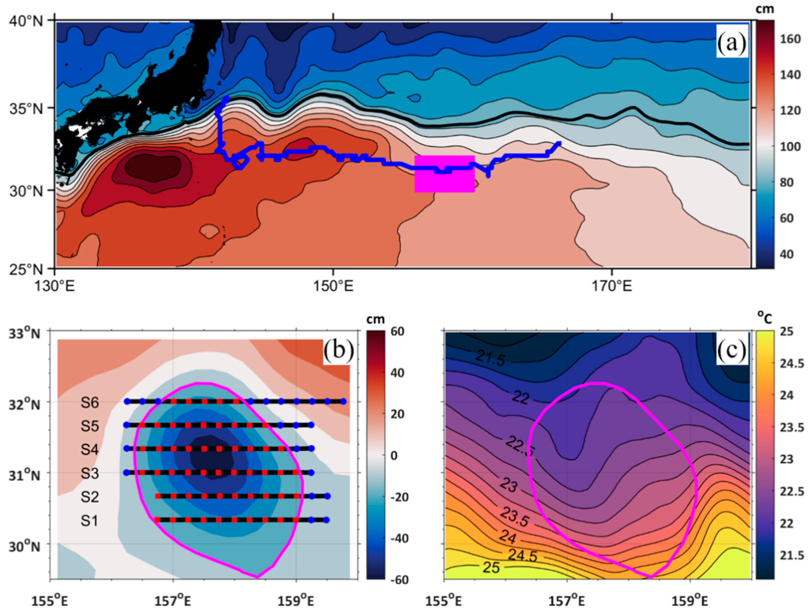
The mesoscale eddy investigated in the present study initially formed at the location (166.375° E, 32.875° N) on January 23, 2014, when it pinched off from the southward curved Kuroshio Extension. The minimum SLA, the intensity and the radius of the newly formed eddy are −18.7 cm, 13 cm and 66.8 km, respectively. The intensity is defined here to be the magnitude of the difference between the SLA of the eddy boundary and the minimum SLA inside the eddy. It is known that the mesoscale eddy formed due to the meandering of the Kuroshio path usually has a longer lifetime and larger size than other eddies [34]. After pinching off from the Kuroshio Extension, the cold mesoscale eddy moved westward for 1150 km, nearly parallel to the contour of the mean dynamic height with an average velocity of 2.51 cm s−1. When encountering the Izu-Ogasawara Ridge in early July of 2015, the eddy swirled and moved northward along the topography. The eddy eventually dissipated at 35° N in August (Figure 1a). The region of the survey is located at the Shatsky Rise, where the eddy was at its mature stage and maintained an intensification tendency (with larger amplitude). The minimum SLA, the intensity and the radius at this time were −57 cm, 48.8 cm and 144.4 km, respectively.
The eddy boundary is defined by the outermost closed contour of SLA, which was −0.1 m for the eddy (Figure 1b). The surface geometric pattern exhibited a northwest-southeast oriented ellipse. The red and blue squares indicate the XCTD stations inside and outside the mesoscale eddy. The minimum SLA in the eddy center was −0.58m and the amplitude was 0.48m. All the surface characteristics show that the field observed eddy is one of the strongest eddies.
The eddy’s SST patterns are usually grouped into dipole and monopole [35]. For the cyclonic eddy in the present study, the SST primarily demonstrated a dipole pattern with cold advection in the west and warm advection in the east. The lowest and highest temperatures were 21.8 °C and 24.9 °C, respectively (Figure 1c). Other satellite data of the surface observations are either absent (sea surface salinity, SSS) or only partly available (chlorophyll concentration) during the period of the field experiment.
3.2. Temperature
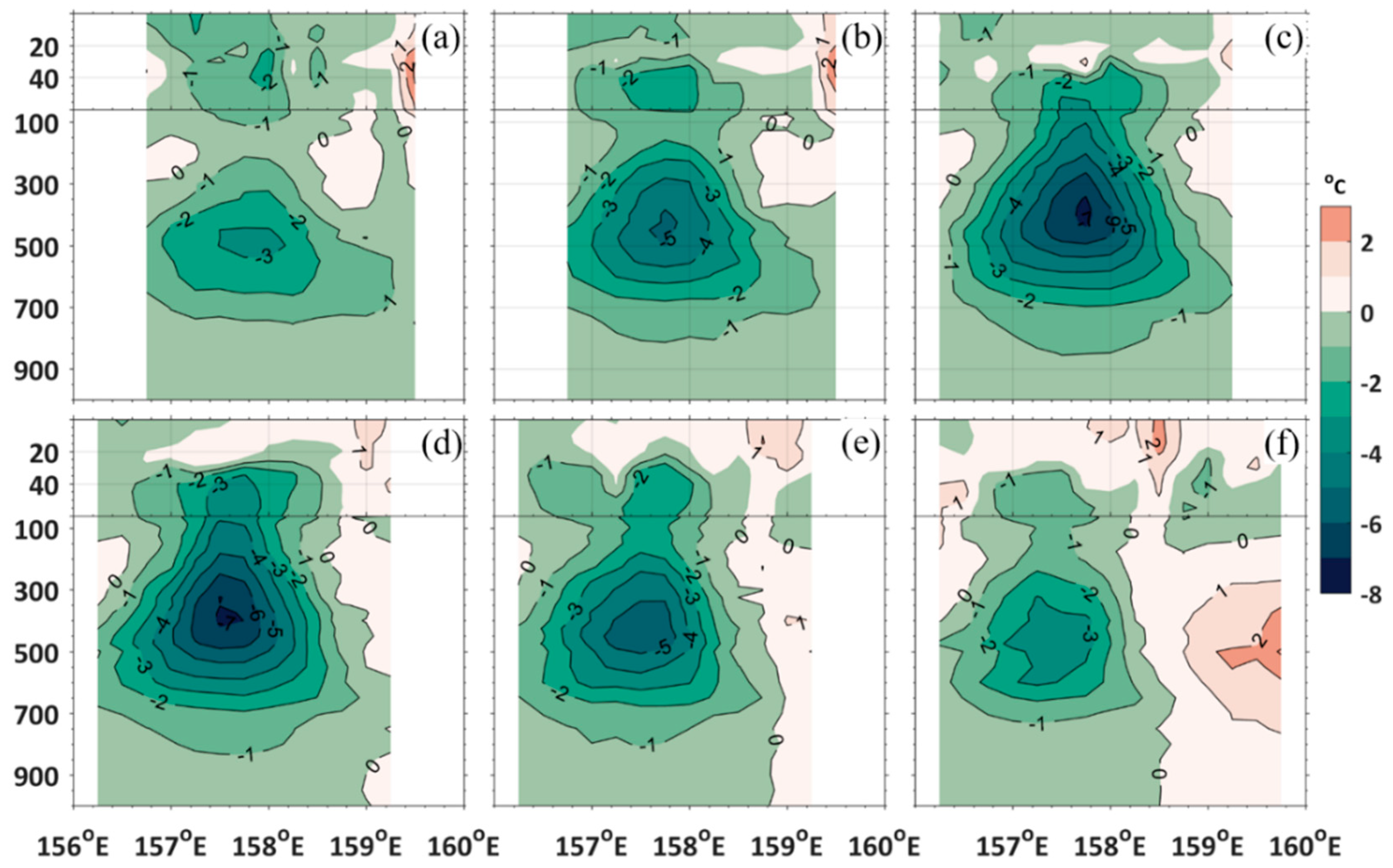
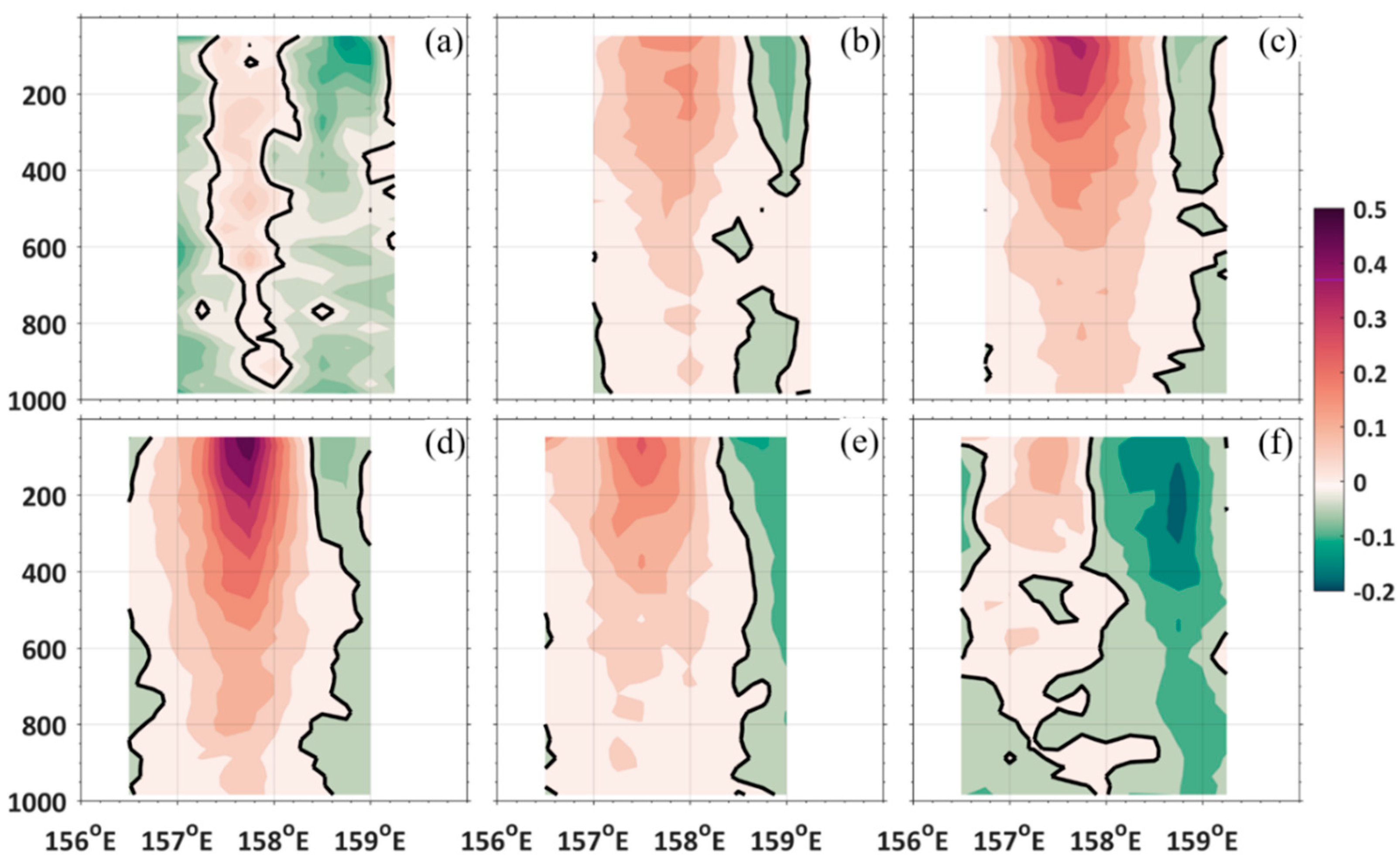
Figure 2 shows temperature anomalies in all the six sections. The main feature is that there was a cone structure with a relative flat bottom located near 500–700 m depth and an apex located near 30–40 m depth. The maximum negative temperature anomaly was up to −7.3 °C occurred near 400 m depth, which is almost half of the climatological temperature (−13.5 °C). The cold anomaly in the thermocline shows that this cyclonic eddy is the subsurface-intensified type of eddy [25]. It can also be found that there existed a warm anomaly in the eastern part of the eddy. This warm anomaly was also manifest in the satellite SST (Figure 1c).
3.3. Salinity
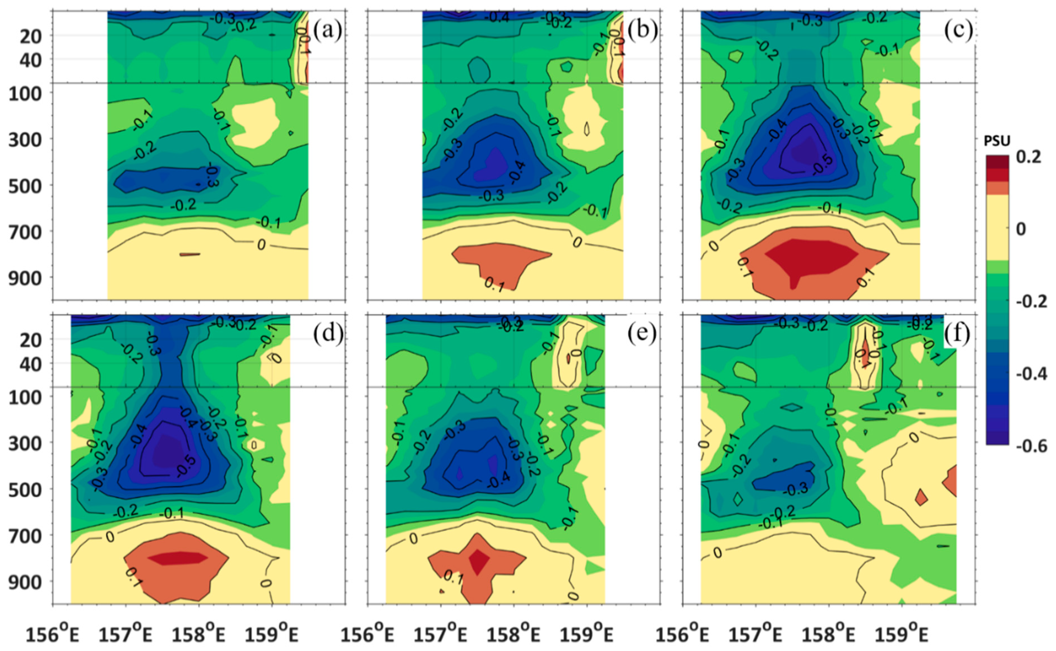
The salinity anomalies are shown in Figure 3. The main feature is that there was a vertical dipole structure with negative anomalies in the upper layer and positive anomalies in the lower layer with the boundary between them located at 700-800 m. The freshest anomaly was −0.61 PSU occurred at 350 m depth and the saltiest anomaly is 0.11 PSU occurred at 800 m depth. Note that consistent fresh anomalies existed in the subsurface, which was connected to the main core below the subsurface.
3.4. Currents
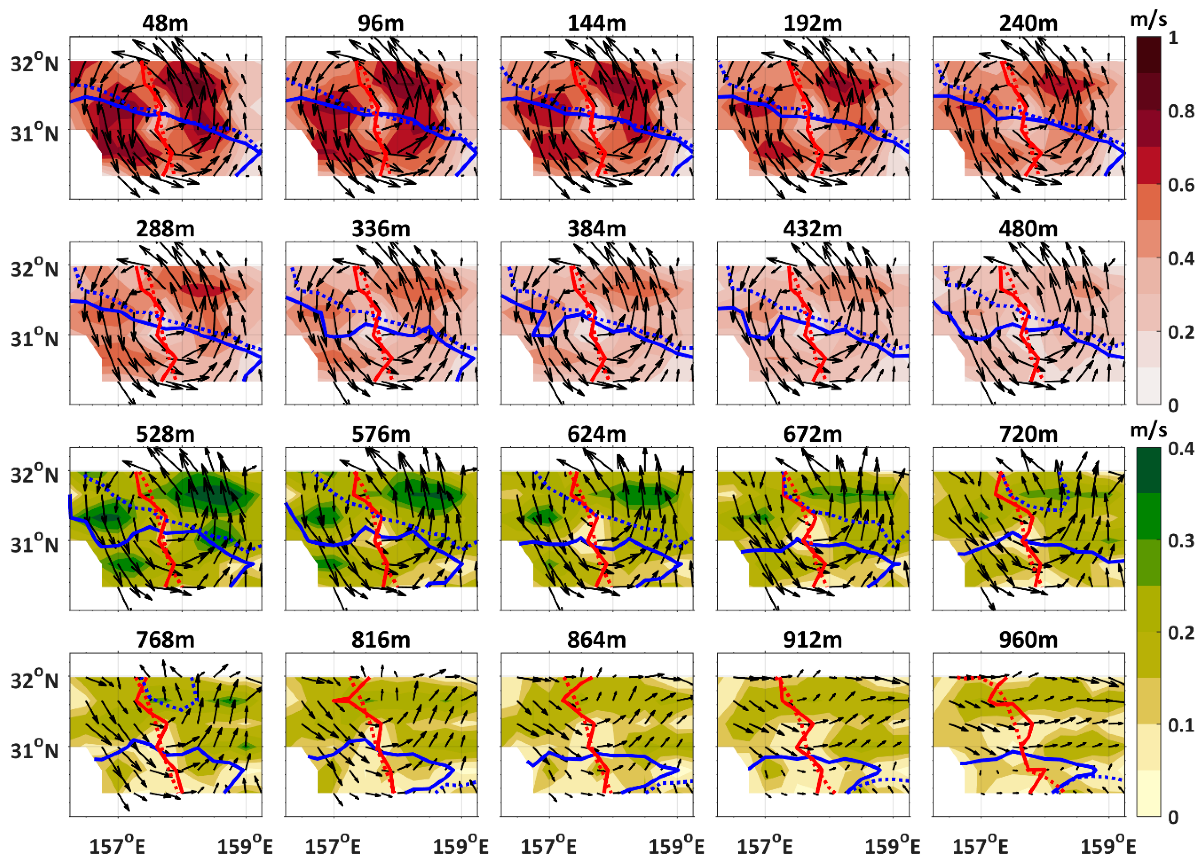
Figure 4 shows the velocities observed by the 38 kHz ADCP at various depths. It can be found that the cyclonic pattern penetrated down to 900 m depth with an equivalent barotropic structure (commonly used in meteorology). The minimum velocity occurred near the center at 48 m depth with the value of only 0.22 m s−1 and the velocity increased outward. The maximum velocity was found in the northeastern and southwestern parts, with the value of nearly 0.90 m s−1 at 48 m depth. Note that only about 5% of the eddies have a velocity larger than 0.4 m s−1 [1] and thereby the above result implies that the eddy observed in the field campaign of the present study is one of the strongest eddies in the ocean. The velocity is asymmetric both in zonal and meridional directions. The blue line in Figure 4 is the dividing line between westward flow to its north and eastward flow to its south. However, note that the dividing line is not strictly zonal but slants a little to the north-south direction. The red line in Figure 4 is the meridional dividing line between southward flow to its east and northward flow to its west. Again, this line is not strictly zonal but slants a little to the east-west direction. Moreover, the zonal dividing line became more zonal with depth increasing.
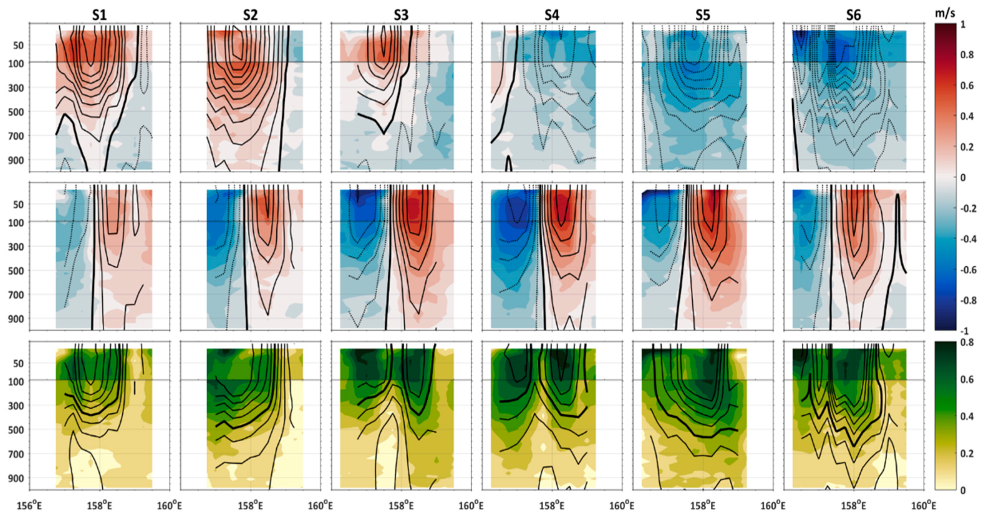
Figure 5 shows vertical distributions of observed zonal and meridional velocities and their magnitudes at various depths, respectively. The zonal currents are mainly eastward (S1, S2 and S3 sections) in the southern and westward (S4, S5 and S6 sections) in the northern part. The meridional currents exhibit a significant barotropic structure with the contour of zero velocity located near 158° E. The magnitude of the velocity demonstrates two large cores in the S3 and S4 sections, where are the kernel of the cyclonic eddy.
4. Thermohaline Impact
4.1. Mixed Layer
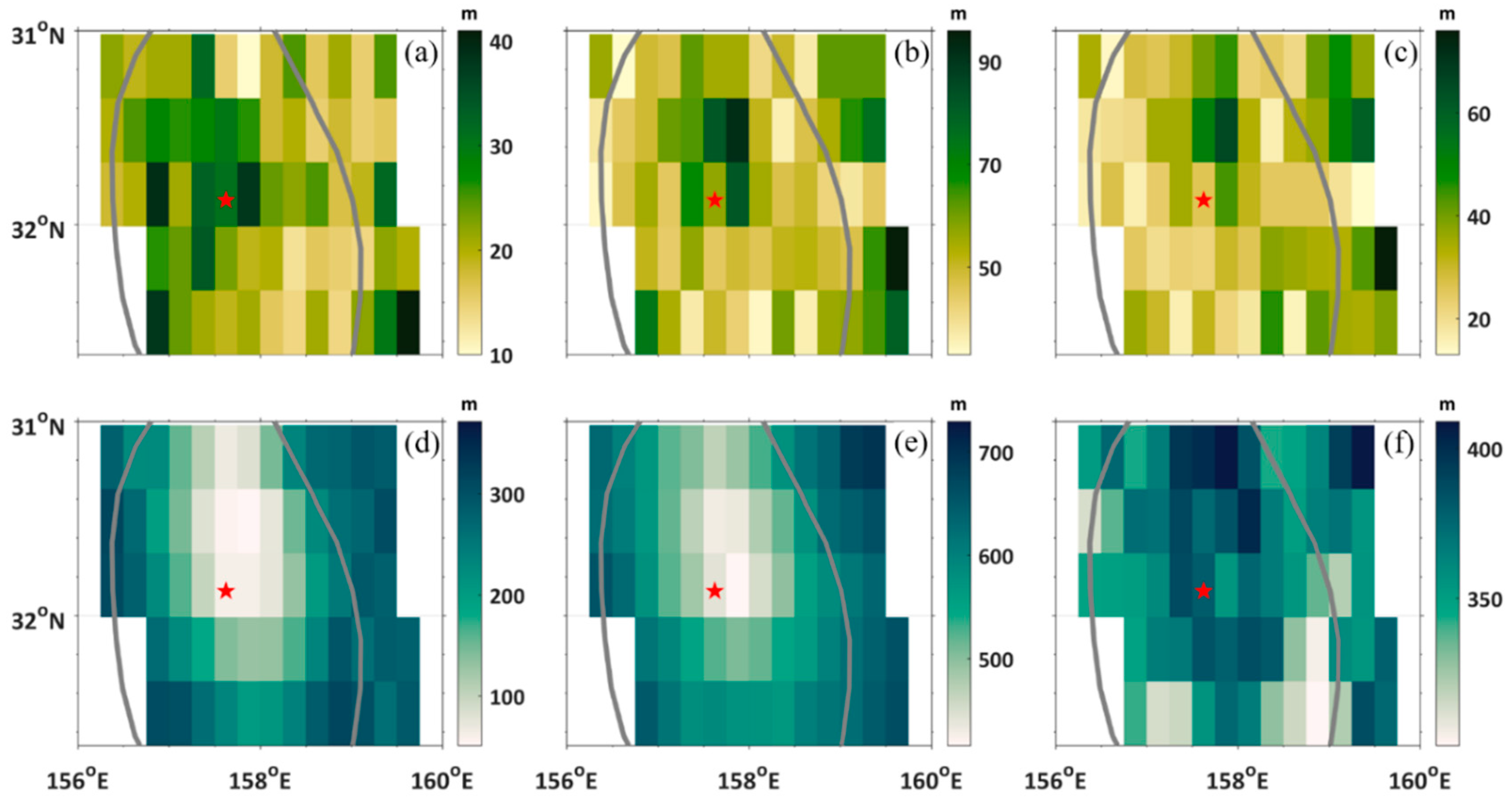
The mixed layer is characterized by nearly uniform properties such as temperature and salinity throughout the layer. Mesoscale eddies can significantly modulate spatial and temporal evolution of the mixed layer [36,37]. The mixed layer depth (MLD) is a layer in which active turbulence is assumed to be mixed and homogeneous to a certain level. Two criteria are often used to identify the MLD: (1) the temperature change from the ocean surface to the MLD should be 0.5 °C; (2) the density change from the ocean surface to the MLD should be 0.125 kg m−3. Spatial averages of MLDs determined by the two criteria are 21.0 m and 22.0 m, respectively. They show similar spatial distributions and thus only the first criterion is presented here. The MLD was deep in the eddy center (40 m) and thin in the periphery (Figure 6a). The deep MLD in the center of the cyclonic eddy is inconsistent with the general conclusion that MLD is shallow in cyclonic eddies and deep in anticyclonic eddies [11,12,36,37]. The reason is that the downwelling process driven by the anticyclonic wind stress mediated by the mesoscale eddy deepens the MLD in the interior of the eddy. More details are given in Section 6.1.
4.2. Thermocline
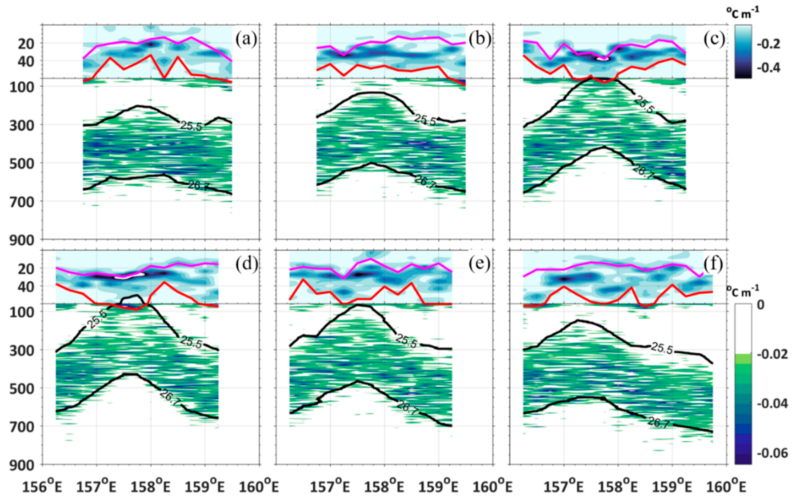
The thermocline is the transition layer between the mixed layer at the surface and the deep water layer, in which temperature decreases rapidly. The seasonal thermocline is determined by the criterion of , where is the vertical gradient of temperature. Figure 7 (upper portion) shows that the mean depth of seasonal thermocline is 54 m and the deepest one is 92 m, which is located around the eddy center. The thickness of the seasonal thermocline is thicker near the eddy center, which can be up to 66 m, which is twice larger than the average.
The criterion of is adopted to identify the permanent thermocline. Figure 7 (lower portion) shows that the permanent thermocline is distributed along the isopycnals. Thus, the potential density kg m−3 and 26.7 kg m−3 are also set to be the upper and lower boundaries of the permanent thermocline. The mean depths of the upper and lower boundaries of the permanent thermocline are 254 m and 582 m, respectively and the mean thickness of the permanent thermocline is 329 m. It can also be found that the closer to the center, the more elevated of the permanent thermocline. The shallowest depth of the upper boundary is 66 m, which is in conjunction with the seasonal thermocline. Far away from the center, the depths of the upper and lower boundary both become deeper with the values of 413 m and 729 m, respectively. The thickest permanent thermocline is located at the northern part of the eddy with a value of 350 m. Outward from the thickest permanent thermocline, the layer becomes thinner and the smallest thickness is only 271 m. Due to the impact of the eddy, the permanent thermocline is uplifted by about 300 m and its thickness is increased by 100 m. Note that for the near-surface intensification of baroclinic modes, altimeters primarily reflect the first baroclinic mode and thus the motion of the main thermocline [38], enabling the use of satellite-derived SLA data to infer subsurface isopycnal displacements [39]. The depressed SLA (Figure 1b) and elevated thermocline (Figure 7) demonstrate a reverse relationship between them.
4.3. STMW
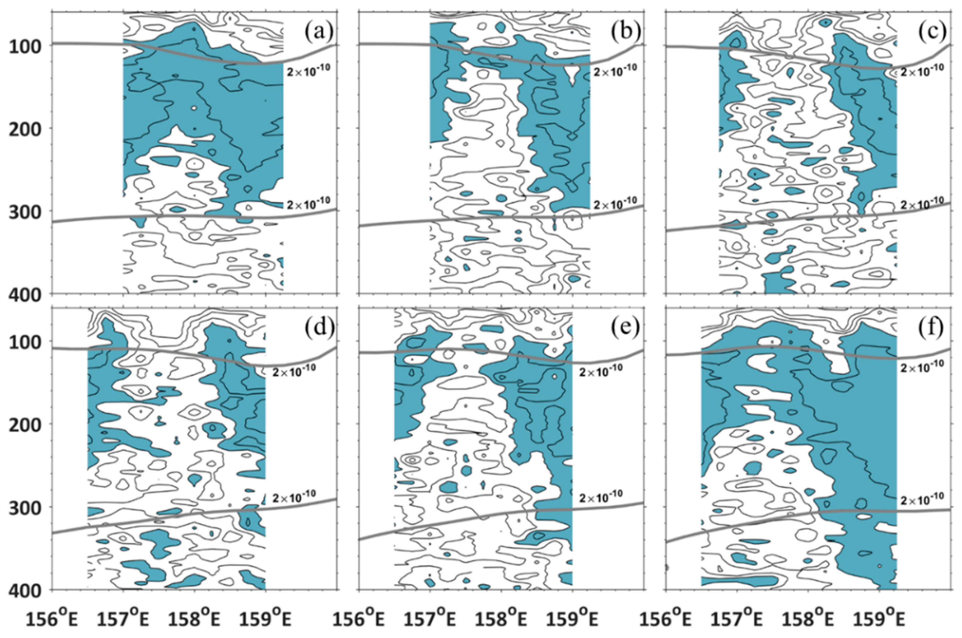
In the North Pacific, the subtropical mode water formed in the deep mixed layer in late winter because of intense convection is known as STMW [40]. STMW is significantly modulated by mesoscale eddies and thick (thin) STMW is co-located with anticyclonic (cyclonic) eddies [31,41,42]. The potential vorticity is used to identify STMW, which is defined as [43]:
where is the Coriolis frequency, is the mean potential density, which is 1026 kg m—3. The criterion that , a potential density between 25.2 and 25.5 and below the mixed layer, is used to define STMW.
The climatological STMW is distributed at about 100–320 m depth to the west of the eddy, while it is compressed upward in the eastern side and located at about 150–275 m depth (Figure 8). In the marginal area of the eddy, the STMW distribution is almost the same as the climatology, except that it is shallower in the western side and deeper in the eastern side. Inside the eddy, STMW weakens and almost vanishes in the center of the eddy. (Figure 8c,d and Figure 9a,b).
The STMW is sandwiched between the seasonal and permanent thermoclines (Figure 8), which can be represented by 25.3 and 25.5 , respectively. Closer to the center, the STMW becomes shallower. In the core of the eddy, the permanent thermocline is in conjunction with the seasonal thermocline and the STMW vanishes. The thin STMW within the cyclonic eddy is consistent with results of the previous studies [44].
The STMW intensity is employed to quantify the cyclonic eddy impact on the STMW. The intensity is defined as:
where is the upper (lower) boundary encompassing the STMW layer with . The results show that the value of decreases inside the eddy, while large values of are distributed in the eastern part, which is out of the eddy, where the warm eddy dominates (Figure 9c). The stable water occupying the original region belongs to the STMW, meaning that the turbulent mixing is depressed in the cyclonic eddy between the seasonal and permanent thermocline.
4.4. NPIW
The North Pacific Intermediate Water (NPIW)—defined as the main salinity minimum along 26.7–26.8 in the subtropical North Pacific [45]—is supposed to be affected by mesoscale eddies [46]. The climatological NPIW is distributed at about 650 m depth with the upper and lower boundaries located at 620 m and 700 m depths, respectively. In the eastern part of the eddy, the observed NPIW is close to its climatological state. The primary impact of the eddy is to uplift the NPIW (Figure 10). Closer to the center, the NPIW becomes shallower. Along the sections S3 and S4, the upper boundary is as shallow as 420 m depth. The mean thickness of the NPIW is 46 m inside the eddy, which is close to the thickness of 43 m outside the eddy (Figure 9d–f).
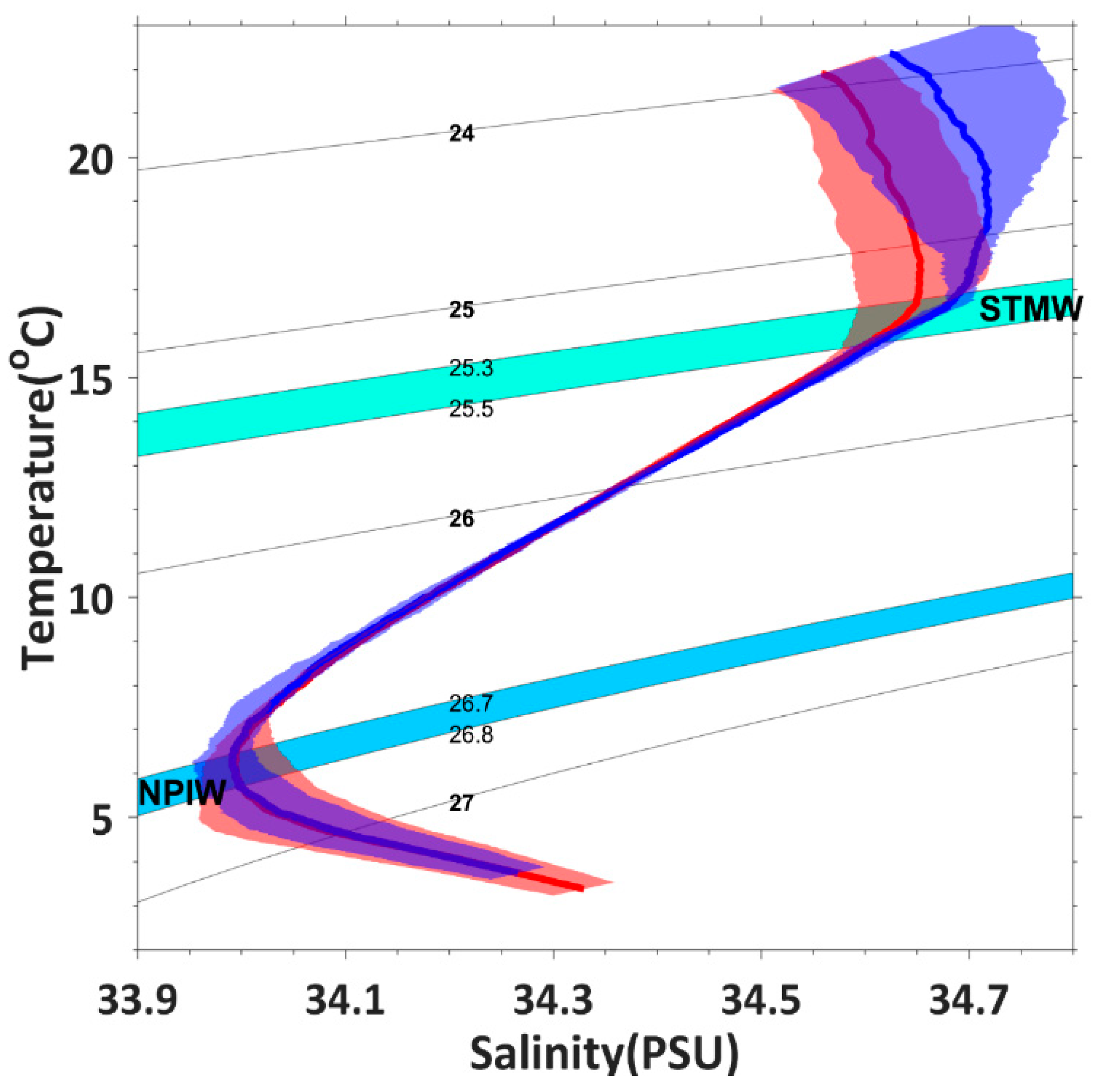
The impact of the cyclonic eddy on the thermohaline structure is summarized in the T/S diagram (Figure 11). The tracers, such as temperature and salinity, are transported along the isopycnals. In the mixed layer and the seasonal thermocline, temperature is colder and salinity is fresher inside the eddy. The SMMW enclosed by the isopycnals of 25.3 and 25.5 is thick outside and thin inside. For the NPIW, the salinity along the isopycnals of 26.7–26.8 is almost the same inside and outside the NPIW with the values of 34.0 PSU and 33.9 PSU, respectively.
5. Dynamic Impact
5.1. Geostrophy
The mesoscale eddies contain the majority of the oceanic kinetic energy and the remaining question to answer is how the mesoscale eddies in geostrophic balance transfer energy to smaller scales, where the energy can be dissipated irreversibly. It is believed that ageostrophic motions play a critical role in this process [47]. Thus, it is important to examine the degree of the geostrophy. The geostrophic currents are calculated by the following algorithm:
where and are the zonal and meridional geostrophic currents, is the gravitational acceleration, is the dynamic height, which is calculated from the temperature and salinity [48]. The geostrophic current represents the baroclinic part of the absolute velocity, which should be included in the barotropical part. There are two commonly used approaches to derive the barotropical currents [49]. One is to consider the barotropical velocities as the depth-averaged flow; the other is to separate the flow into a depth-independent component equal to the geostrophic flow at the bottom and a depth-dependent component equal to the geostrophic flow referenced to zero at the bottom. In this study, the valid measured depth of XCTD is 1000 m. The geostrophic velocity under 1000 m is absent. In order to make up for this gap, the averages of measured by the 38 kHz ADCP between the 900–1000 m, specifically in the layers of 912 m, 936 m, 960 m and 984 m, are added to the geostrophic parts. Thus, the absolute geostrophic currents are derived by the sum of and .
The absolute geostrophic currents are displayed in Figure 5, which shows that the zonal and meridional components and magnitudes of the geostrophic currents match well with the observed flows. This is especially true for the meridional component. The zonal differences are large, as shown in Figure 4, in which the contour of the observed zero zonal flow gradually changes to east-west direction with increasing depth. In contrast, the geostrophic flow direction remains almost unchanged with increasing depth but the speed decreases rapidly.
The relation between the absolute geostrophic and observed flows are quantified by skill (), which is defined as:
where is the absolute velocity, is the observed velocity by the 38 kHz ADCP, the overbar is the observed average at various depths. ranges between and 1 and high values indicate that geostrophic and observed velocities are well correlated and of the same magnitude. The skill is presented in Figure 12a.
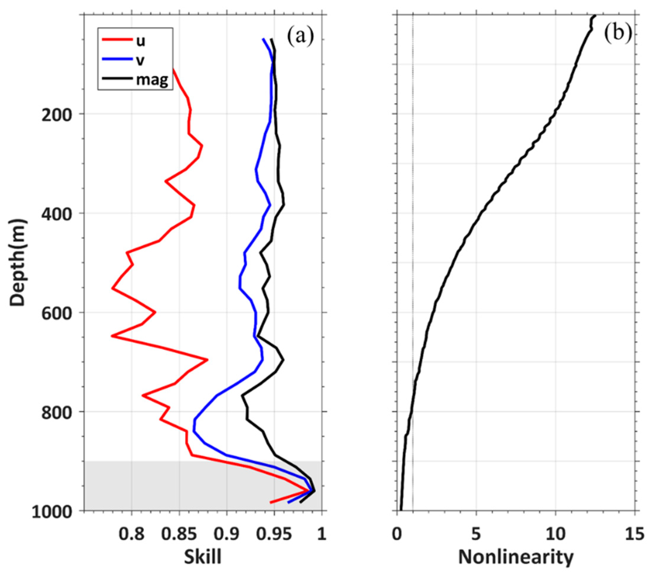
The absolute geostrophic currents can well reproduce the observed values, especially the magnitude. is about 0.98 in the reference layer and decreases with increasing depth. At 48 m, the value of is 0.95. The mean value of is 0.95 for the velocity magnitude at levels above the reference depth and the zonal and meridional components are 0.84 and 0.92, respectively. The value of is 0.89 in the layer between 700–900 m depths, which is relatively low. Compared with the meridional component, the observed values of zonal geostrophic current are less well reproduced, especially in the layer between 480-648 m depths, where the value of is less than 0.8. The mismatch pattern between the zonal geostrophic component and observed currents can also be found in Figure 4 and Figure 5.
5.2. Nonlinearity
Nonlinear eddies tend to trap the fluid contained in their interiors, which can be maintained over long time periods, depending on their evolution and exchange with the surrounding water masses [1,24]. The degree of nonlinearity of a mesoscale eddy is characterized by the ratio of rotational speed () to translational speed (). When > 1, the feature is nonlinear, which allows the eddy to maintain a coherent structure as it propagates. The average translational velocity is cm s−1, which is roughly the same as the value derived by Reference [50] with a latitude-dependent amplification factor [51]. The rotational speed is defined by the maximum of the average geostrophic speeds along all of the closed contours of dynamic height () inside the eddy. The strongest nonlinearity is 12.5 and the nonlinearity weakens with increasing depth, which implies that the eddy can trap materials effectively (Figure 12b). The nonlinearity is bigger than 1 until 780 m depth.
Another measurement of nonlinearity is the normalized vorticity (), which is defined as the relative vorticity () normalized by the Coriolis parameter (). This parameter compares the local relative vorticity of the eddy with the planetary vorticity, also known as the Rossby number (). Compared with the parameter , can reveal the detailed horizontal structure of the eddy. The maximum is 0.4, which is located near the eddy center at 48 m depth (Figure 13). With increasing depth, the normalized vorticity decreases, which demonstrates that the nonlinearity weakens with increasing depth.
6. Discussion
6.1. Eddy-Wind Interaction
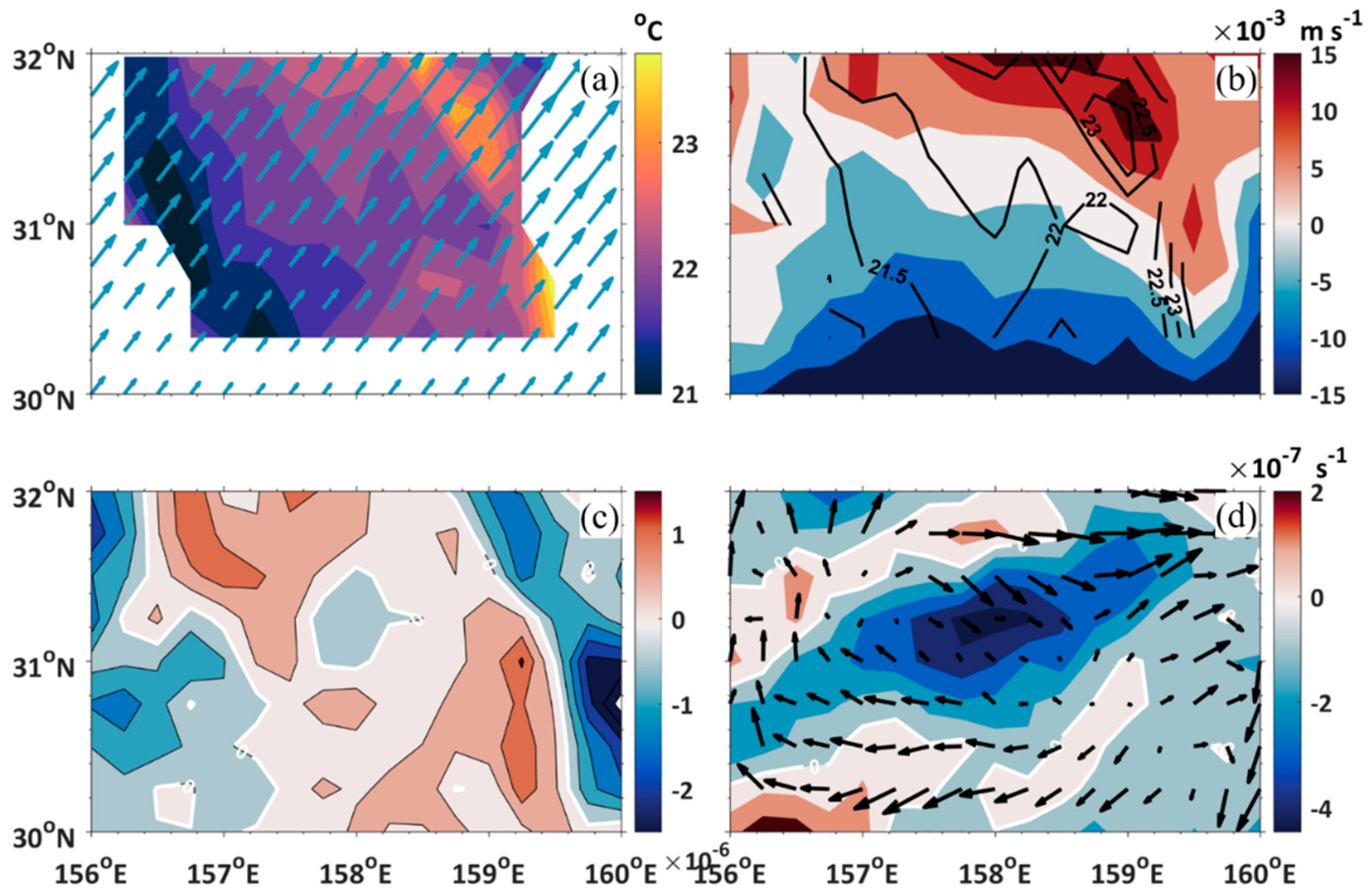
At oceanic fronts and eddies, the positive correlation between SST and wind speed reflects the fact that the ocean drives the atmosphere, which is contrary to the situation for large-scale climate modes, in which the atmosphere drives the oceans [52]. Cooler ocean temperatures tend to stabilize the marine atmospheric boundary layer, decoupling it from winds aloft. Conversely, warmer ocean temperatures tend to destabilize the boundary layer, thereby decreasing the vertical wind shear. The net effect of the ocean is to increase surface wind speed over warmer water and decrease it over colder water, leading to measurable differences in wind stress, wind stress curl and therefore Ekman pumping [53,54]. The positive correlation between SST and wind stress is clearly presented in Figure 14a. The wind stress is prevalent in the southwest direction and changes a little to the north direction in the left lower and west direction in the top right corner. The wind stress magnitudes (represented by the lengths of the vectors) are relatively large over warm water and small over cold water. The positive correlation is demonstrated by the coupled pattern between the wind stress anomaly and SST (referred to as the 5 m depth water temperature) shown in Figure 14b. Their linear correlation coefficient is 0.47 (which is significant at the level of 0.05). The relation between wind stress and SST is particularly remarkable in the top right corner, where positive wind stress coexists with warm water.
According to the downward momentum transport mechanism, the divergence is linearly correlated with the downwind component of the SST gradient [53,55]. The positive divergence is distributed along the eddy with a northwestern-southeastern direction. The correlation coefficient between the divergence and the downwind SST gradient is 0.56 (which is significant at the level of 0.05), which favors the downwind momentum mixing mechanism as an explanation.
Moreover, there is a direct effect on the wind stress caused by eddy-driven surface currents, which can be conveniently expressed in the form of bulk parameterization of the wind stress as [56]
where is the wind stress, is the density of the air, is the drag coefficient, and are the 10-m wind speed and the surface current speed, respectively. That is, stronger stress occurs on the flank of the eddy, where the wind direction is opposite to the direction of the underlying water flow, while lower stress occurs on the flank of the eddy where the wind and the water flow are in the same direction. The anticyclonic wind stress induces negative wind stress curl and downwelling process (Figure 14d), which dampens the eddy-induced upwelling [5].
6.2. Dipole Temperature vs. Monopole Salinity
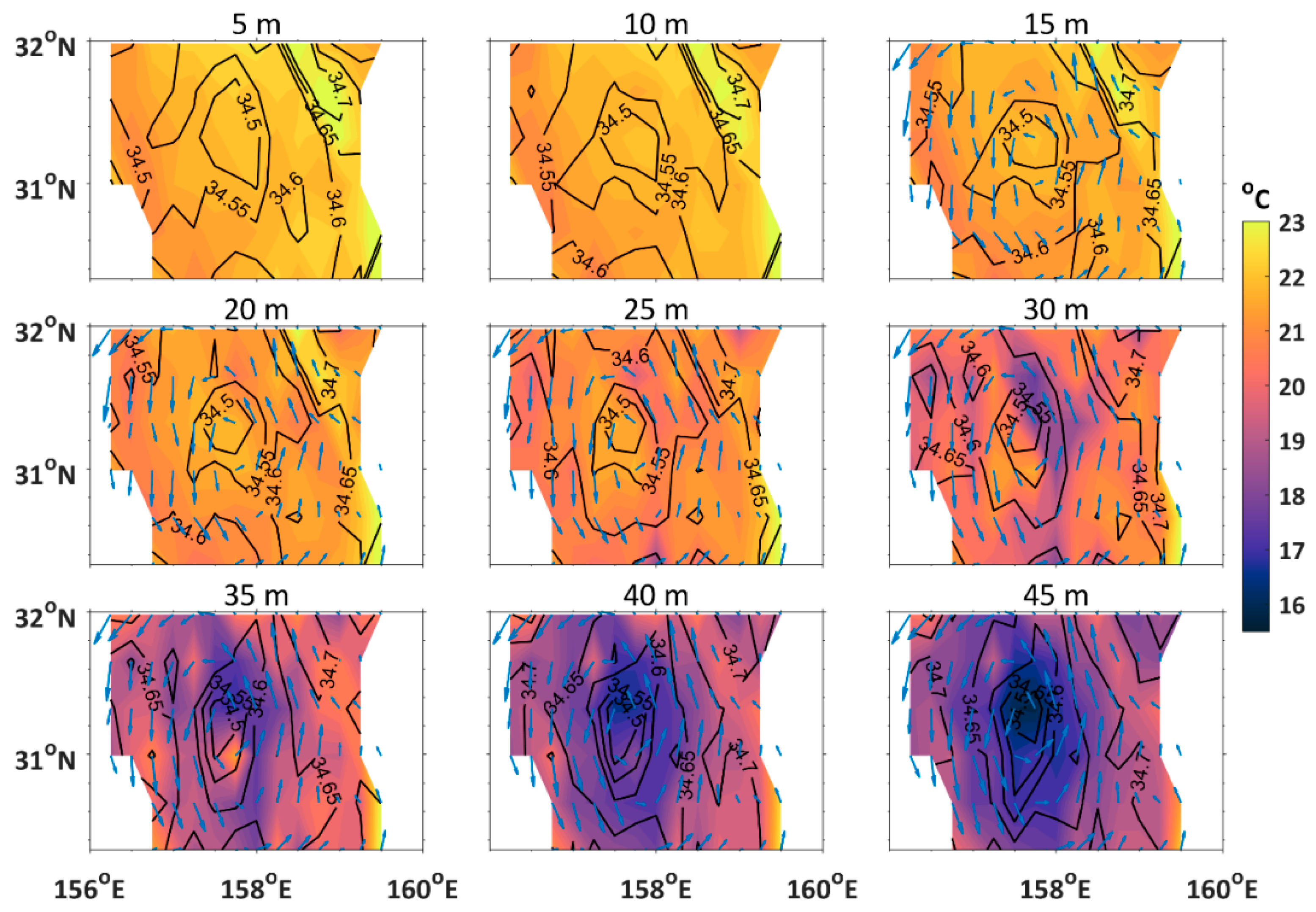
Wind-induced mixing and upwelling associated with the eddy exert profound influences on upper ocean circulations and biological processes. Observations of the sea water temperature and salinity in the upper layer show different features (Figure 15). The spatial distribution pattern of temperature resembles the eddy’s shape, which is oriented along the southwest-northeast direction. Warm temperature is found in the top right corner, while cold temperature is located on the bottom left. This dipole structure is also observed on the surface by the satellite (Figure 1c). With increasing depth, this dipole pattern gradually changes into a monopole structure until 40m depth, which is the base of the mixed layer. Comparatively, the salinity shows a monopole in the whole mixed layer with low-salinity water located in the center of the mixed layer. The 3D structures of temperature and salinity show that the dipole pattern of temperature and the monopole pattern of salinity are not only manifest on the surface (SST and SSS) but also maintain in the mixed layer.
The mechanisms by which mesoscale eddies influence tracers like temperature, salinity and chlorophyll are grouped into horizontal (e.g., stirring and trapping) and vertical (e.g., eddy pumping and eddy-induced Ekman pumping) processes [24,57]. In order to clarify the effects of different processes, the mixed layer temperature diagnostic equation [58] is implemented for further analysis in the present study. The equation is expressed by:
where is the MLD, which is 40 m, is the temperature in the mixed layer, is the velocity vector, is the Heaviside function, is the entrainment velocity, is the surface heat flux into the ocean, is the heat flux at the mixed-layer base, is horizontal mixing coefficient. Because there is no observational heat flux on eddy resolving scale in this study, the heat flux term is not considered. In addition, the dissipation term is also not considered here. The vertical pumping driven by the Ekman wind stress is considered, whereas the eddy pumping induced by the displacement of isopycnals is ignored because the isopycnals in the mixed layer were relatively flat (Figure 7). Note that the coefficient is set to 0 (1) when downwelling (upwelling) process occurs. However, the eddy-induced Ekman pumping associated with spatial variations in wind stress is taken as a bulk impact on the water, thus is set to 1. Hence, the slab mixed-layer model is reduced to the balance between the time variation and advective and vertical terms.
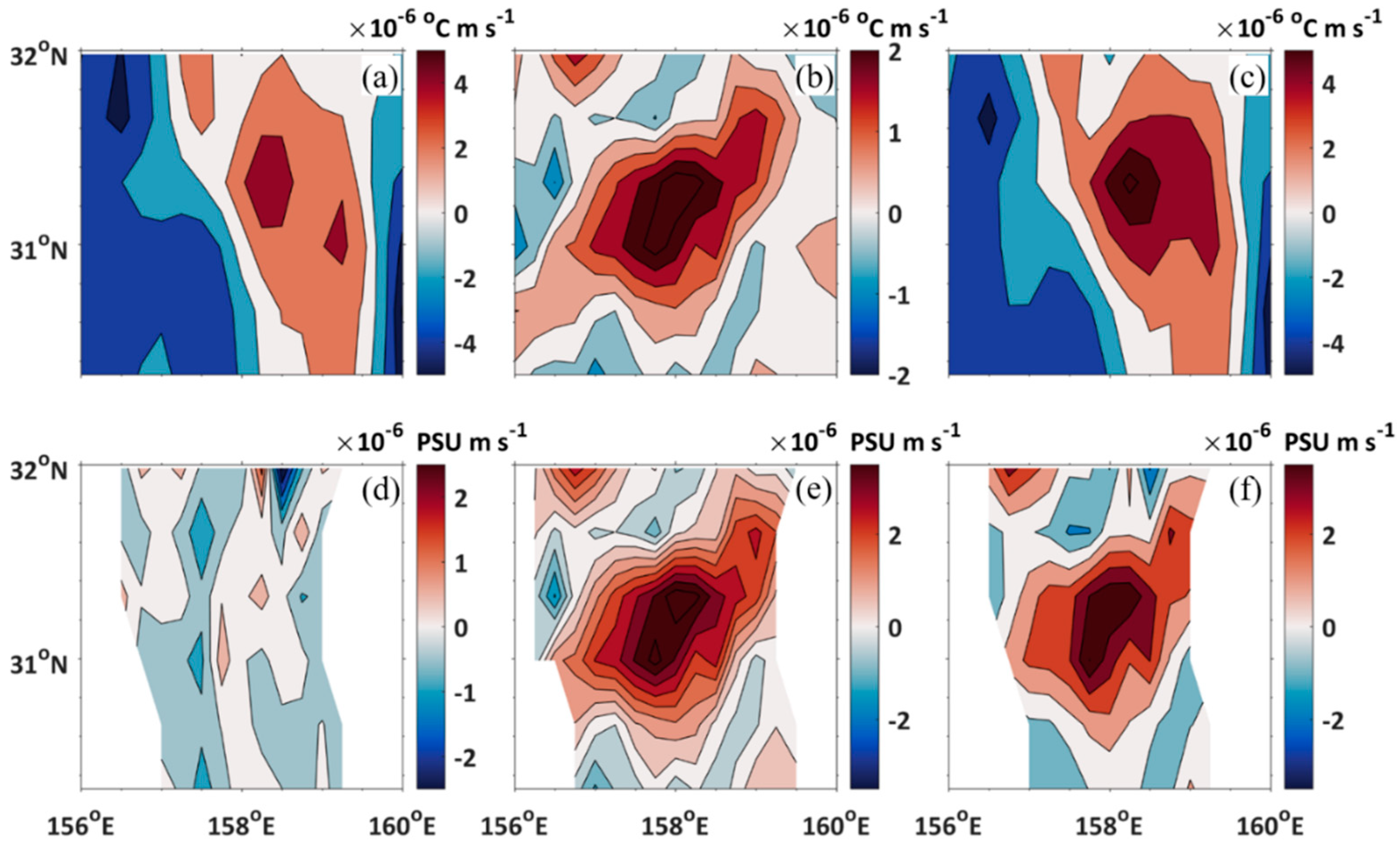
The diagnostic results show that there is warm advection in the right half part and cold advection in the left half part of the cyclonic flow (Figure 16a). Meanwhile, the downwelling induced by the wind stress increases MLD in the core of the eddy (Figure 6a). Besides, it also causes a monopole structure of temperature in the eddy core (Figure 16b). The sum of the horizontal and vertical processes are displayed in Figure 16c, which shows that, instead of the Ekman upwelling, the horizontal advection actually dominates the temperature variation and results in the dipole structure of the temperature in the mixed layer.
Similarly, the equation for SSS [59] is given by,
where is the salinity, is the evaporation, is the precipitation. The mixing process and freshwater flux are ignored. Similar to the equation for temperature, the equation for SSS is balanced by the local rate and advective and vertical components. Contrary to the situation for temperature variability, the eddy-induced Ekman pumping dominates the horizontal transport of salinity (Figure 16d–f). The difference between the temperature and salinity structures in the mixed layer is attributed to the ambient environment. Because the temperature is warm in the south and cool in the north, the advective process transports the cold water southward and warm water northward, which results in the dipole structure of temperature. However, there is no distinct salinity difference between the northern and southern regions. Instead of horizontal advection, the eddy-induced Ekman pumping is prominent for the spatial distribution of salinity, which leads to the monopole structure of salinity.
7. Conclusions
The Kuroshio Extension region has the largest sea level variability on mesoscale time scale in the extratropical North Pacific Ocean, which is one of the regions with the most intense air-sea heat exchange across the globe. Due to severe sea conditions and long distance between the oceans and the continents, it is hard to conduct field campaigns to measure ocean conditions and high-resolution sampling by ships is even harder to achieve. In this study, a strong cyclonic eddy in the Kuroshio Extension was detected at the end of June 2014 based on observations of XCTD instruments and shipboard ADCP combined with satellite observations SLA, SST and wind stress were collected.
The cyclonic eddy was generated by the meander of the Kuroshio path, which had a long lifetime and large size. The field experiment was conducted when the eddy was crossing the Shatsky Rise. Vertically, the temperature anomaly showed a cone structure with the bottom located at 500–700 m depth and the apex was at 30–40 m depth. The salinity anomaly demonstrated a dipole pattern with negative anomalies in the upper layer and positive anomalies in the lower layer with the boundary located at 700-800 m depth. Horizontally, the temperature and salinity in the mixed layer are dipole and monopole structures, respectively. The flow field was observed by the shipboard ADCP instruments and the maximum was close to 0.90 m s−1 at 48 m depth. Comparing with the composite results of Argo profiles in the Kuroshio Extension region [12,60], the observed 3D anatomy shows more details and new results, such as vertical monopole and dipole structures of temperature and salinity anomaly, horizontal dipole and monopole structures of temperature and salinity in the mixed layer and the equivalent barotropic flow structure.
The thermohaline and dynamic impact of the cyclonic eddy is studied. The deepest MLD of 40 m was found near the center of the eddy. The deep MLD location in the cyclonic eddy is inconsistent with the general conclusion from other studies. The reason is that the downwelling process driven by the anticyclonic wind stress that was generated by the eddy deepened the MLD. Both the seasonal and permanent thermoclines became shallower because of the upward doming of the isopycnals. The impact of eddy could uplift the permanent thermocline by about 300 m and increased its thickness by 100 m. For the relatively less stratified water mass, the STMW weakened in the eddy and even dissipated near the center; for the NPIW, the salinity had no significant change except certain increases due to the doming of the isopycnals. Benefiting from the grid observations, the geostrophic currents are calculated and compared with the observed velocities measured by the ADCP measurements. The geostrophic balance relation is approximately set up by calculating the explained skill. The nonlinearity quantified by the ratio of rotational speed divided to the translational speed is 12.5 in the surface and maintains until 780 m depth. The nonlinearity can also be expressed by the normalized vorticity, which is defined by the relative vorticity divided by the Coriolis frequency. The maximum normalized vorticity is 0.4 near the center at 48 m depth. Both the nonlinearity and the geostrophic balance degraded with increasing depth. As an intense eddy, the influence of the eddy on the stratification is significant, that the seasonal thermocline is strengthened, the permanent thermocline is uplifted, the STMW weakens and dissipates in the eddy center and NPIW is upraised along the isopycnals. The results show that not only the dynamic state of the KE and the overlying atmospheric conditions [31], the intense eddy can also disrupt the SMTW among their formation and evolution.
The influence of mesoscale SST on wind stress is studied by using satellite observations. The wind stress increases above the warm SST, which implies that the ocean forces the atmosphere. Cold SST induces positive wind stress divergence and negative wind stress curl. The different horizontal temperature and salinity structures in the mixed layer is discussed. The two distinct mechanisms, that is, horizontal transport and upwelling induced by the eddy mediated wind stress, are demonstrated by using the simple model. The results show that the horizontal and vertical transports are responsible for the dipole temperature pattern and monopole salinity pattern, respectively.
The cyclonic eddy was sampled in the high-resolution field experiment. However, the eddy was mixed with the ambient environment and the 3D structure of the eddy changed during the entire life cycle. More observations need to be conducted in the future.
Author Contributions
Conceptualization, X.C. and Y.Z.; methodology, Y.Z. and C.D.; validation, Y.Z., X.C. and C.D.; formal analysis, Y.Z.; investigation, X.C. and Y.Z.; resources, Y.Z.; writing—original draft preparation, Y.Z.; writing—review and editing, Y.Z., X.C. and C.D.; visualization, Y.Z.; supervision, X.C. and C.D.; project administration, X.C. and C.D.; funding acquisition, C.D.
Funding
This research was funded by the National Key Research Program of China (2017YFA0604100, 2016YFA0601803), National Natural Science Foundation of China (41406003, 41490643), China Postdoctoral Science Foundation funded project (2013M541959), Jiangsu Provincial Natural Science Foundation (BK20130064), the National Programme on Global Change and Air-Sea Interaction (GASI-03-IPOVAI-05) and the foundation of China Ocean Mineral Resources R & D Association (DY135-E2-2-02, DY135-E2-3-01).
Acknowledgments
The authors appreciate the scientists and crews of R/V Xiangyanghong 10 for their contribution to the field experiment. We are grateful to AVISO (http://www.aviso.altimetry.fr/) for providing us with the SLA data, GHRSST, UKMO and MyOcean for providing us with the UKMO SST data.
Conflicts of Interest
The authors declare no conflict of interest.
References
- Chelton, D.B.; Schlax, M.G.; Samelson, R.M. Global observations of nonlinear mesoscale eddies. Prog. Oceanogr. 2011, 91, 167–216. [Google Scholar] [CrossRef]
- Group, M. The mid-ocean dynamics experiment. Deep Sea Res. 1978, 25, 859–910. [Google Scholar]
- McWilliams, J.; Brown, E.; Bryden, H.; Ebbesmeyer, C.; Elliott, B.; Heinmiller, R.; Hua, B.L.; Leaman, K.; Lindstrom, E.; Luyten, J. The local dynamics of eddies in the Western North Atlantic. Springer 1983, 92–113. [Google Scholar] [CrossRef]
- Benitez-Nelson, C.R.; Bidigare, R.R.; Dickey, T.D.; Landry, M.R.; Leonard, C.L.; Brown, S.L.; Nencioli, F.; Rii, Y.M.; Maiti, K.; Becker, J.W. Mesoscale eddies drive increased silica export in the subtropical Pacific Ocean. Science 2007, 316, 1017–1021. [Google Scholar] [CrossRef]
- McGillicuddy, D.J.; Anderson, L.A.; Bates, N.R.; Bibby, T.; Buesseler, K.O.; Carlson, C.A.; Davis, C.S.; Ewart, C.; Falkowski, P.G.; Goldthwait, S.A. Eddy/wind interactions stimulate extraordinary mid-ocean plankton blooms. Science 2007, 316, 1021–1026. [Google Scholar] [CrossRef]
- Pascual, A.; Ruiz, S.; Olita, A.; Troupin, C.; Claret, M.; Casas, B.; Mourre, B.; Poulain, P.-M.; Tovar-Sanchez, A.; Capet, A. A multiplatform experiment to unravel meso-and submesoscale processes in an intense front (AlborEx). Front. Mar. Sci. 2017, 4, 39. [Google Scholar] [CrossRef]
- Zhang, Z.; Qiu, B.; Tian, J.; Zhao, W.; Huang, X. Latitude-dependent finescale turbulent shear generations in the Pacific tropical-extratropical upper ocean. Nat. Commun. 2018, 9, 4086. [Google Scholar] [CrossRef]
- Roemmich, D.; Johnson, G.C.; Riser, S.; Davis, R.; Gilson, J.; Owens, W.B.; Garzoli, S.L.; Schmid, C.; Ignaszewski, M. The Argo Program: Observing the global ocean with profiling floats. Oceanography 2009, 22, 34–43. [Google Scholar] [CrossRef]
- Castelao, R.M. Mesoscale eddies in the South Atlantic Bight and the Gulf Stream recirculation region: vertical structure. J. Geophys. Res. Ocean. 2014, 119, 2048–2065. [Google Scholar] [CrossRef]
- Chaigneau, A.; Le Texier, M.; Eldin, G.; Grados, C.; Pizarro, O. Vertical structure of mesoscale eddies in the eastern South Pacific Ocean: A composite analysis from altimetry and Argo profiling floats. J. Geophys. Res. Ocean. 2011, 116. [Google Scholar] [CrossRef]
- He, Q.; Zhan, H.; Cai, S.; He, Y.; Huang, G.; Zhan, W. A New Assessment of Mesoscale Eddies in the South China Sea: Surface Features, Three-Dimensional Structures and Thermohaline Transports. J. Geophys. Res. Ocean. 2018, 123, 4906–4929. [Google Scholar] [CrossRef]
- Sun, W.; Dong, C.; Wang, R.; Liu, Y.; Yu, K. Vertical structure anomalies of oceanic eddies in the Kuroshio Extension region. J. Geophys. Res. Ocean. 2017, 122, 1476–1496. [Google Scholar] [CrossRef]
- Yang, G.; Wang, F.; Li, Y.; Lin, P. Mesoscale eddies in the northwestern subtropical Pacific Ocean: Statistical characteristics and three-dimensional structures. J. Geophys. Res. Ocean. 2013, 118, 1906–1925. [Google Scholar] [CrossRef]
- Xu, L.; Li, P.; Xie, S.-P.; Liu, Q.; Liu, C.; Gao, W. Observing mesoscale eddy effects on mode-water subduction and transport in the North Pacific. Nat. Commun. 2016, 7, 10505. [Google Scholar] [CrossRef] [PubMed]
- Zhang, Z.; Tian, J.; Qiu, B.; Zhao, W.; Chang, P.; Wu, D.; Wan, X. Observed 3D structure, generation and dissipation of oceanic mesoscale eddies in the South China Sea. Sci. Rep. 2016, 6. [Google Scholar] [CrossRef] [PubMed]
- Rudnick, D.L. Ocean research enabled by underwater gliders. Annu. Rev. Mar. Sci. 2016, 8, 519–541. [Google Scholar] [CrossRef] [PubMed]
- Kolodziejczyk, N.; Testor, P.; Lazar, A.; Echevin, V.; Krahmann, G.; Chaigneau, A.; Gourcuff, C.; Wade, M.; Faye, S.; Estrade, P. Subsurface Fine-Scale Patterns in an Anticyclonic Eddy Off Cap-Vert Peninsula Observed From Glider Measurements. J. Geophys. Res. Ocean. 2018, 123, 6312–6329. [Google Scholar] [CrossRef]
- Shu, Y.; Chen, J.; Li, S.; Wang, Q.; Yu, J.; Wang, D. Field-observation for an anticyclonic mesoscale eddy consisted of twelve gliders and sixty-two expendable probes in the northern South China Sea during summer 2017. Sci. China Earth Sci. 2018, 62, 451–458. [Google Scholar] [CrossRef]
- Barceló-Llull, B.; Sangrà, P.; Pallàs-Sanz, E.; Barton, E.D.; Estrada-Allis, S.N.; Martínez-Marrero, A.; Aguiar-González, B.; Grisolía, D.; Gordo, C.; Rodríguez-Santana, Á. Anatomy of a subtropical intrathermocline eddy. Deep Sea Research Part I: Oceanographic Research Papers. ScienceDirect 2017, 124, 126–139. [Google Scholar]
- Hu, J.; Gan, J.; Sun, Z.; Zhu, J.; Dai, M. Observed three-dimensional structure of a cold eddy in the southwestern South China Sea. J. Geophys. Res. Ocean. 2011, 116, C05016. [Google Scholar] [CrossRef]
- Kurczyn, J.; Beier, E.; Lavín, M.; Chaigneau, A.; Godínez, V. Anatomy and evolution of a cyclonic mesoscale eddy observed in the northeastern Pacific tropical-subtropical transition zone. J. Geophys. Res. Ocean. 2013, 118, 5931–5950. [Google Scholar] [CrossRef]
- Garreau, P.; Dumas, F.; Louazel, S.; Stegner, A.; Le Vu, B. High-Resolution Observations and Tracking of a Dual-Core Anticyclonic Eddy in the Algerian Basin. J. Geophys. Res. Ocean. 2018, 123, 9320–9339. [Google Scholar] [CrossRef]
- Flierl, G.; McGillicuddy, D.J. Mesoscale and submesoscale physical-biological interactions. The Sea 2002, 12, 113–185. [Google Scholar]
- McGillicuddy, D.J., Jr. Mechanisms of physical-biological-biogeochemical interaction at the oceanic mesoscale. Annu. Rev. Mar. Sci. 2016, 8, 125–159. [Google Scholar] [CrossRef] [PubMed]
- Pegliasco, C.; Chaigneau, A.; Morrow, R. Main eddy vertical structures observed in the four major Eastern Boundary Upwelling Systems. J. Geophys. Res. Ocean. 2015, 120, 6008–6033. [Google Scholar] [CrossRef]
- Zhang, Z.; Li, P.; Xu, L.; Li, C.; Zhao, W.; Tian, J.; Qu, T. Subthermocline eddies observed by rapid-sampling Argo floats in the subtropical northwestern Pacific Ocean in Spring 2014. Geophys. Res. Lett. 2015, 42, 6438–6445. [Google Scholar] [CrossRef] [Green Version]
- Li, C.; Zhang, Z.; Zhao, W.; Tian, J. A statistical study on the subthermocline submesoscale eddies in the northwestern P acific O cean based on A rgo data. J. Geophys. Res. Ocean. 2017, 122, 3586–3598. [Google Scholar] [CrossRef]
- Pelland, N.A.; Eriksen, C.C.; Lee, C.M. Subthermocline eddies over the Washington continental slope as observed by Seagliders, 2003–2009. J. Phys. Oceanogr. 2013, 43, 2025–2053. [Google Scholar] [CrossRef]
- Zhang, Z.; Liu, Z.; Richards, K.; Shang, G.; Zhao, W.; Tian, J.; Huang, X.; Zhou, C. Elevated diapycnal mixing by a sub-thermocline eddy in the western equatorial Pacific. Geophys. Res. Lett. 2019, 46, 2628–2636. [Google Scholar] [CrossRef]
- Dong, C.; Lin, X.; Liu, Y.; Nencioli, F.; Chao, Y.; Guan, Y.; Chen, D.; Dickey, T.; McWilliams, J.C. Three-dimensional oceanic eddy analysis in the Southern California Bight from a numerical product. J. Geophys. Res. Ocean. 2012, 117. [Google Scholar] [CrossRef] [Green Version]
- Qiu, B.; Chen, S.; Hacker, P. Effect of mesoscale eddies on subtropical mode water variability from the Kuroshio Extension System Study (KESS). J. Phys. Oceanogr. 2007, 37, 982–1000. [Google Scholar] [CrossRef]
- Xu, L.; Xie, S.P.; Liu, Q.; Liu, C.; Li, P.; Lin, X. Evolution of the North Pacific subtropical mode water in anticyclonic eddies. J. Geophys. Res. Ocean. 2017, 122, 10118–10130. [Google Scholar] [CrossRef]
- Von Schuckmann, K.; Gaillard, F.; Le Traon, P.Y. Global hydrographic variability patterns during 2003–2008. J. Geophys. Res. Ocean. 2009, 114, C09007. [Google Scholar] [CrossRef]
- Ji, J.; Dong, C.; Zhang, B.; Liu, Y.; Zou, B.; King, G.P.; Xu, G.; Chen, D. Oceanic Eddy Characteristics and Generation Mechanisms in the Kuroshio Extension Region. J. Geophys. Res. Ocean. 2018, 123, 8548–8567. [Google Scholar] [CrossRef]
- Frenger, I.; Münnich, M.; Gruber, N.; Knutti, R. Southern O cean eddy phenomenology. J. Geophys. Res. Ocean. 2015, 120, 7413–7449. [Google Scholar] [CrossRef] [Green Version]
- Gaube, P.; McGillicuddy, D.J.; Moulin, A.J. Mesoscale Eddies Modulate Mixed Layer Depth Globally. Geophys. Res. Lett. 2018, 46. [Google Scholar] [CrossRef]
- Hausmann, U.; McGillicuddy, D.J.; Marshall, J. Observed mesoscale eddy signatures in Southern Ocean surface mixed-layer depth. J. Geophys. Res. Ocean. 2017, 122, 617–635. [Google Scholar] [CrossRef] [Green Version]
- Wunsch, C. The vertical partition of oceanic horizontal kinetic energy. J. Phys. Oceanogr. 1997, 27, 1770–1794. [Google Scholar] [CrossRef]
- McGillicuddy, D.J., Jr.; Robinson, A.; Siegel, D.; Jannasch, H.; Johnson, R.; Dickey, T.; McNeil, J.; Michaels, A.; Knap, A. Influence of mesoscale eddies on new production in the Sargasso Sea. Nature 1998, 394, 263. [Google Scholar] [CrossRef]
- Sugimoto, S.; Hanawa, K.; Watanabe, T.; Suga, T.; Xie, S.-P. Enhanced warming of the subtropical mode water in the North Pacific and North Atlantic. Nat. Clim. Chang. 2017, 7, 656–658. [Google Scholar] [CrossRef]
- Oka, E.; Suga, T.; Sukigara, C.; Toyama, K.; Shimada, K.; Yoshida, J. “Eddy resolving” observation of the North Pacific subtropical mode water. J. Phys. Oceanogr. 2011, 41, 666–681. [Google Scholar] [CrossRef]
- Shi, F.; Luo, Y.; Xu, L. Volume and Transport of Eddy-Trapped Mode Water South of the Kuroshio Extension. J. Geophys. Res. Ocean. 2018, 123. [Google Scholar] [CrossRef]
- Nishikawa, S.; Tsujino, H.; Sakamoto, K.; Nakano, H. Effects of mesoscale eddies on subduction and distribution of subtropical mode water in an eddy-resolving OGCM of the western North Pacific. J. Phys. Oceanogr. 2010, 40, 1748–1765. [Google Scholar] [CrossRef]
- Kouketsu, S.; Tomita, H.; Oka, E.; Hosoda, S.; Kobayashi, T.; Sato, K. The role of meso-scale eddies in mixed layer deepening and mode water formation in the western North Pacific. In New Developments in Mode-Water Research; Springer: New York, NY, USA, 2011; pp. 59–73. [Google Scholar]
- Talley, L.D. Distribution and formation of North Pacific intermediate water. J. Phys. Oceanogr. 1993, 23, 517–537. [Google Scholar] [CrossRef]
- Qiu, B.; Chen, S. Effect of decadal Kuroshio Extension jet and eddy variability on the modification of North Pacific Intermediate Water. J. Phys. Oceanogr. 2011, 41, 503–515. [Google Scholar] [CrossRef]
- Zhang, Z.; Qiu, B. Evolution of Submesoscale Ageostrophic Motions Through the Life Cycle of Oceanic Mesoscale Eddies. Geophys. Res. Lett. 2018, 45, 11847–11855. [Google Scholar] [CrossRef]
- Tomczak, M.; Godfrey, J.S. Regional Oceanography: An Introduction; Pergamon: Oxford, UK, 1994. [Google Scholar]
- Peña-Molino, B.; Rintoul, S.; Mazloff, M. Barotropic and baroclinic contributions to along-stream and across-stream transport in the A ntarctic C ircumpolar C urrent. J. Geophys. Res. Ocean. 2014, 119, 8011–8028. [Google Scholar] [CrossRef]
- Chelton, D.B.; DeSzoeke, R.A.; Schlax, M.G.; El Naggar, K.; Siwertz, N. Geographical variability of the first baroclinic Rossby radius of deformation. J. Phys. Oceanogr. 1998, 28, 433–460. [Google Scholar] [CrossRef]
- Qiu, B.; Chen, S. Decadal variability in the large-scale sea surface height field of the South Pacific Ocean: Observations and causes. J. Phys. Oceanogr. 2006, 36, 1751–1762. [Google Scholar] [CrossRef]
- Small, R.; Xie, S.; O’Neill, L.; Seo, H.; Song, Q.; Cornillon, P.; Spall, M.; Minobe, S. Air–sea interaction over ocean fronts and eddies. Dyn. Atmos. Ocean. 2008, 45, 274–319. [Google Scholar] [CrossRef]
- Chelton, D.B.; Schlax, M.G.; Freilich, M.H.; Milliff, R.F. Satellite measurements reveal persistent small-scale features in ocean winds. science 2004, 303, 978–983. [Google Scholar] [CrossRef]
- Frenger, I.; Gruber, N.; Knutti, R.; Münnich, M. Imprint of Southern Ocean eddies on winds, clouds and rainfall. Nat. Geosci. 2013, 6, 608. [Google Scholar] [CrossRef]
- Chelton, D.B.; Schlax, M.G.; Samelson, R.M. Summertime coupling between sea surface temperature and wind stress in the California Current System. J. Phys. Oceanogr. 2007, 37, 495–517. [Google Scholar] [CrossRef]
- Seo, H.; Miller, A.J.; Norris, J.R. Eddy–wind interaction in the California Current System: Dynamics and impacts. J. Phys. Oceanogr. 2016, 46, 439–459. [Google Scholar] [CrossRef]
- Gaube, P.; McGillicuddy, D.J., Jr.; Chelton, D.B.; Behrenfeld, M.J.; Strutton, P.G. Regional variations in the influence of mesoscale eddies on near-surface chlorophyll. J. Geophys. Res. Ocean. 2014, 119, 8195–8220. [Google Scholar] [CrossRef] [Green Version]
- Frankignoul, C.; Czaja, A.; L’Heveder, B. Air–sea feedback in the North Atlantic and surface boundary conditions for ocean models. J. Clim. 1998, 11, 2310–2324. [Google Scholar] [CrossRef]
- Delcroix, T.; Cravatte, S.; McPhaden, M.J. Decadal variations and trends in tropical Pacific sea surface salinity since 1970. J. Geophys. Res. Ocean. 2007, 112. [Google Scholar] [CrossRef]
- Dong, D.; Brandt, P.; Chang, P.; Schütte, F.; Yang, X.; Yan, J.; Zeng, J. Mesoscale Eddies in the Northwestern Pacific Ocean: Three-Dimensional Eddy Structures and Heat/Salt Transports. J. Geophys. Res. Ocean. 2017, 122, 9795–9813. [Google Scholar] [CrossRef]
Figure 1.
Surface characteristics. (a) Mean dynamic topography (MDT) in the northwestern North Pacific Ocean. The mean Kuroshio Extension axis is represented as bold black line, which is 120 cm of MDT. The blue line shows the eddy movement trajectory. The overlaid magenta rectangle is the study area (156.25–157.75° E, 30.33–32° N). (b) Sea level anomaly (SLA) and survey stations. Shaded areas indicate the SLA and the magenta line is the −0.1 m contour of SLA, which indicates the boundary of the cyclonic eddy. The black lines are the cruising tracks, from south to north named S1, S2, S3, S4, S5 and S6. The squares overlaid on the tracks are the stations with Expendable conductivity–temperature–depth (XCTD) probes deployed. The red and blue squares indicate the stations inside and outside the eddy based on the eddy boundary. (c) Sea surface temperature observed by the satellite. The magenta line is the boundary as the same in (b).

Figure 2.
Temperature anomalies at the six sections. (a), (b), (c), (d), (e) and (f) are for the sections of S1, S2, S3, S4, S5 and S6, respectively.
Figure 2.
Temperature anomalies at the six sections. (a), (b), (c), (d), (e) and (f) are for the sections of S1, S2, S3, S4, S5 and S6, respectively.

Figure 3.
Same as in Figure 2 but for salinity anomaly.
Figure 3.
Same as in Figure 2 but for salinity anomaly.

Figure 4.
Velocity observed by the 38 kHz shipboard acoustic Doppler current profilers (ADCP) at various depths. Shaded areas show the magnitude of the velocity. Vectors show the flows direction and magnitude. The red and blue full (dotted) lines indicate the zero lines of observed (geostrophic) meridional and zonal velocities, respectively.

Figure 5.
Observed velocity and geostrophic velocity. Shaded areas indicate the observed velocity, which were measured by the 300 kHz and 38 kHz ADCP at depths shallower and deeper than 90 m, respectively. The contours show the geostrophic currents, the solid and dotted lines indicate positive and negative velocities and the black (magenta) thick line is the observed (geostrophic) zero-velocity contour in the upper and middle panels and the 0.4 m s−1 contour in the bottom panel. Zonal velocity in the S1, S2, S3, S4, S5, S6 sections are shown in upper panels from left to right. Meridional velocity in the S1, S2, S3, S4, S5, S6 sections are shown in middle panels from left to right. Velocity magnitude in the S1, S2, S3, S4, S5, S6 sections are shown in bottom panels from left to right.

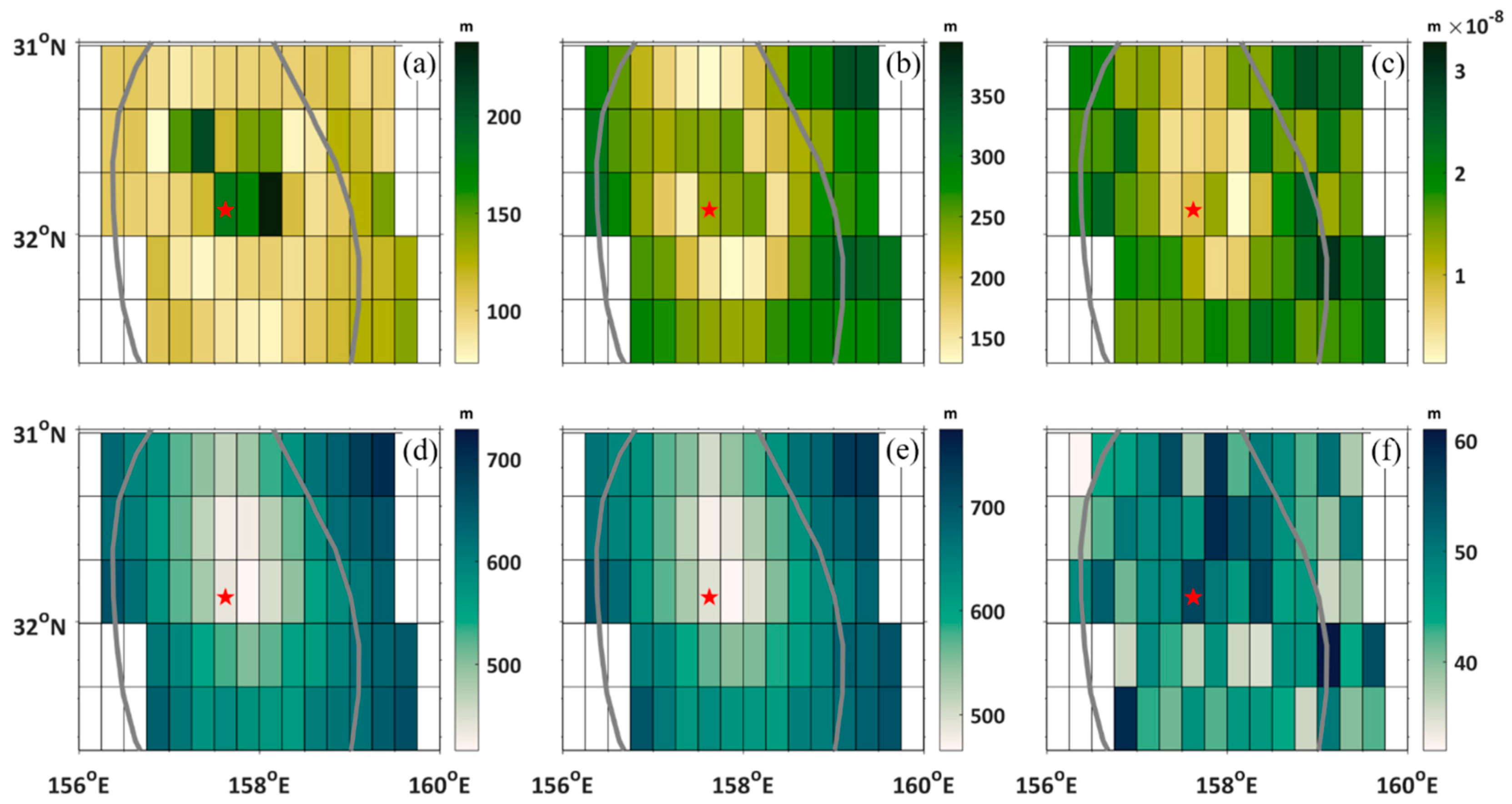
Figure 6.
Mixed layer, seasonal and permanent thermoclines. (a) Mixed layer depth (MLD), which is also the upper boundary of the seasonal thermocline. (b) The bottom of the seasonal thermocline. (c) The thickness of the seasonal thermocline. (d) The depth corresponding to the upper boundary of the permanent thermocline, which is along the contour of 25.5 . (e) The depth corresponding to the lower boundary of the permanent thermocline, which is along the contour of 26.7 . (f) The thickness of the permanent thermocline. The MLD is determined as the depth with temperature change of 0.5 °C from the ocean surface to this depth. The seasonal and permanent thermoclines are determined here by vertical temperature gradients larger than 0.05 and 0.02 , respectively.

Figure 7.
Thermocline. (a), (b), (c), (d), (e) and (f) are for the sections of S1, S2, S3, S4, S5 and S6, respectively. The vertical gradient of temperature () is used to identify the thermocline. larger than 0.05 and 0.02 are deemed to be the seasonal thermocline and permanent thermocline. The magenta and red lines denote the upper and lower boundaries of the seasonal thermocline. The magenta line also shows the MLD. The black lines are the isopycnals of 25.5 and 26.7 , which correspond to the upper and lower boundaries of the permanent thermocline.

Figure 8.
Subtropical Mode Water (STMW). (a), (b), (c), (d), (e) and (f) are for the sections of S1, S2, S3, S4, S5 and S6, respectively. The potential vorticity smaller than is used to identify STMW between 25.3 and 25.5 , which is nattier blue shaded. The gray line denotes the climatological potential vorticity of .

Figure 9.
STMW and North Pacific Intermediate Water (NPIW). (a) Upper and (b) lower boundaries of the STMW. (c) Intensity of the STMW. (d) Upper and (e) lower boundaries of the NPIW. (f) The thickness of the NPIW.
Figure 9.
STMW and North Pacific Intermediate Water (NPIW). (a) Upper and (b) lower boundaries of the STMW. (c) Intensity of the STMW. (d) Upper and (e) lower boundaries of the NPIW. (f) The thickness of the NPIW.

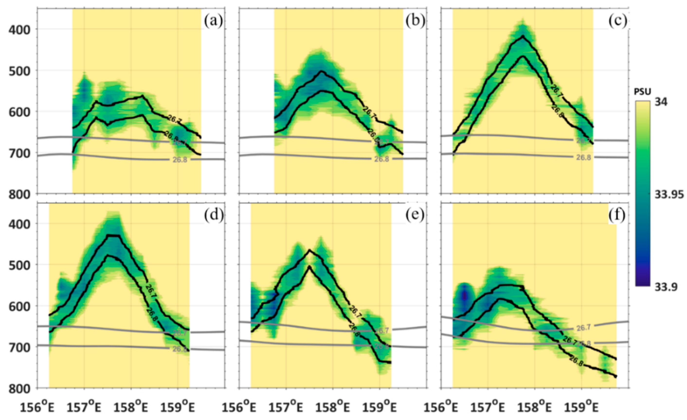
Figure 10.
NPIW. (a), (b), (c), (d), (e) and (f) are for the sections of S1, S2, S3, S4, S5 and S6, respectively. Shaded areas indicate the observed salinity with 33.9PSU-34.0PSU. The black lines indicate 26.7–26.8 , which are used to characterize the range of the NPIW. The gray lines are the climatological isopycnals of 26.7–26.8 .

Figure 11.
Temperature-Salinity diagram. The blue and red lines are the averages of temperature and salinity inside and outside the eddy. The shaded regions are their standard deviations, respectively. The STMW and NPIW are cyan and blue color shaded, which correspond to 25.3 −25.5 and 26.7 −26.8 , respectively.

Figure 12.
(a) The skill of the geostrophic currents. The black, red and blue lines are the magnitude, zonal and meridional velocities, respectively. The grey shaded in the bottom is the barotropical velocity which is added to the geostrophic velocity. (b) Nonlinearity defined by translational speed divided by the rotational speed.

Figure 13.
Vertical relative vorticity scaled by the planetary vorticity. (a), (b), (c), (d), (e) and (f) are for the sections of S1, S2, S3, S4, S5 and S6, respectively. The black line is the zero contour.
Figure 13.
Vertical relative vorticity scaled by the planetary vorticity. (a), (b), (c), (d), (e) and (f) are for the sections of S1, S2, S3, S4, S5 and S6, respectively. The black line is the zero contour.

Figure 14.
(a) The wind stress (vectors) and water temperature (color shaded) at 5 m depth. (b) Wind stress magnitude (shaded) and water temperature (contours). (c) Wind stress divergence. (d) Wind stress curl.
Figure 14.
(a) The wind stress (vectors) and water temperature (color shaded) at 5 m depth. (b) Wind stress magnitude (shaded) and water temperature (contours). (c) Wind stress divergence. (d) Wind stress curl.

Figure 15.
Temperature, salinity and velocity at different depths. Shaded areas indicate temperature. The vectors are velocities measured by the 300 kHz ADCP.
Figure 15.
Temperature, salinity and velocity at different depths. Shaded areas indicate temperature. The vectors are velocities measured by the 300 kHz ADCP.

Figure 16.
Sea Surface Temperature (SST) and Sea Surface Salinity (SSS) diagnoses. (a) SST induced by the advection. (b) SST induced by the Ekman downwelling. (c) SST induced by the sum of the horizontal and vertical processes. (d) SSS induced by the advection. (e) SSS induced by the Ekman upwelling. (f) SSS induced by the sum of the horizontal and vertical processes.

© 2019 by the authors. Licensee MDPI, Basel, Switzerland. This article is an open access article distributed under the terms and conditions of the Creative Commons Attribution (CC BY) license (http://creativecommons.org/licenses/by/4.0/).
Share and Cite
MDPI and ACS Style
Zhang, Y.; Chen, X.; Dong, C. Anatomy of a Cyclonic Eddy in the Kuroshio Extension Based on High-Resolution Observations. Atmosphere 2019, 10, 553. https://doi.org/10.3390/atmos10090553
AMA Style
Zhang Y, Chen X, Dong C. Anatomy of a Cyclonic Eddy in the Kuroshio Extension Based on High-Resolution Observations. Atmosphere. 2019; 10(9):553. https://doi.org/10.3390/atmos10090553
Chicago/Turabian StyleZhang, Yongchui, Xi Chen, and Changming Dong. 2019. "Anatomy of a Cyclonic Eddy in the Kuroshio Extension Based on High-Resolution Observations" Atmosphere 10, no. 9: 553. https://doi.org/10.3390/atmos10090553
Note that from the first issue of 2016, this journal uses article numbers instead of page numbers. See further details here.