Modeling Streamflow Enhanced by Precipitation from Atmospheric River Using the NOAA National Water Model: A Case Study of the Russian River Basin for February 2004


Abstract
:1. Introduction
2. Materials and Methods
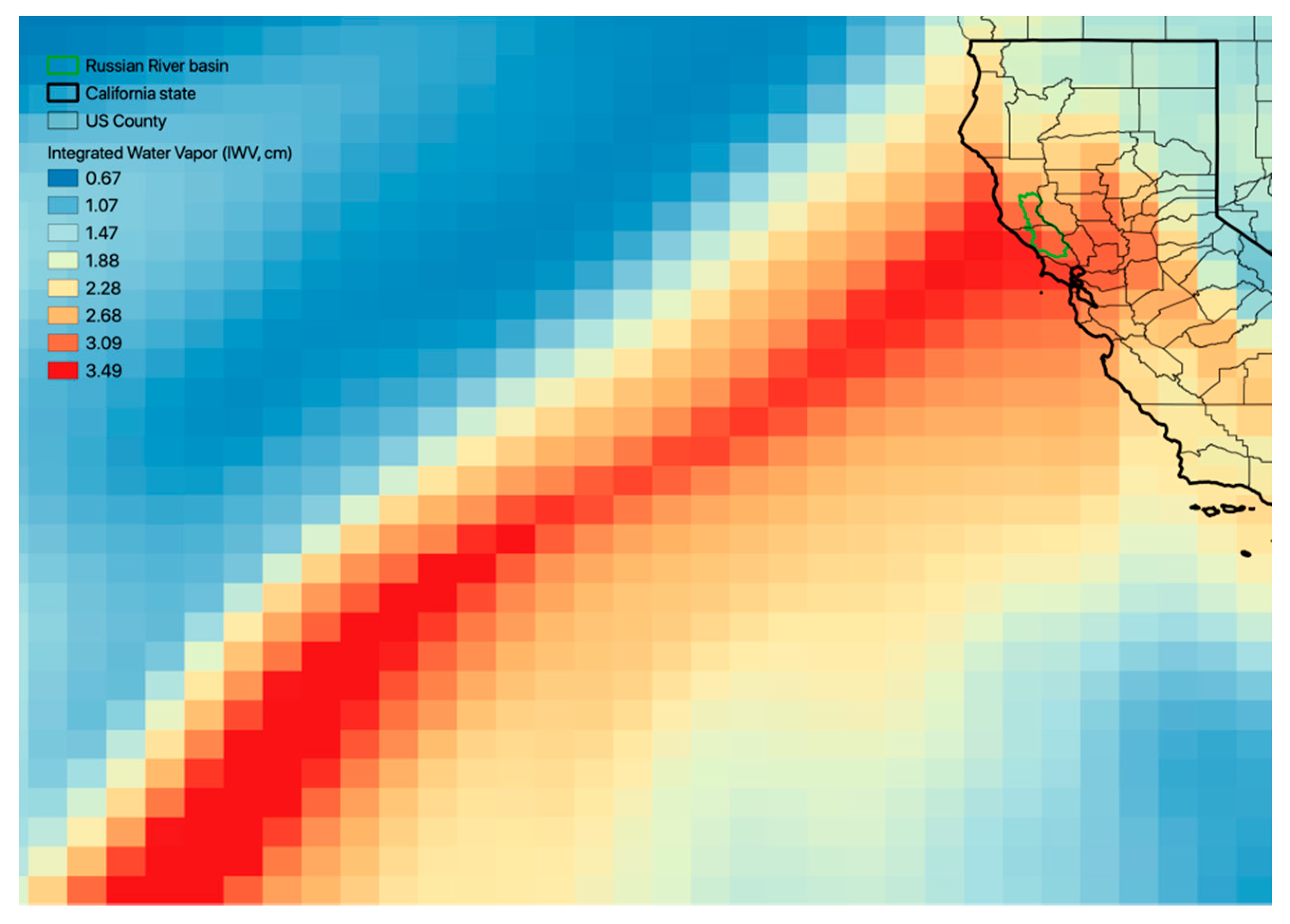
2.1. Atmospheric River
2.2. National Water Model
2.3. Hydrological Products Provided by NWM
2.4. Data
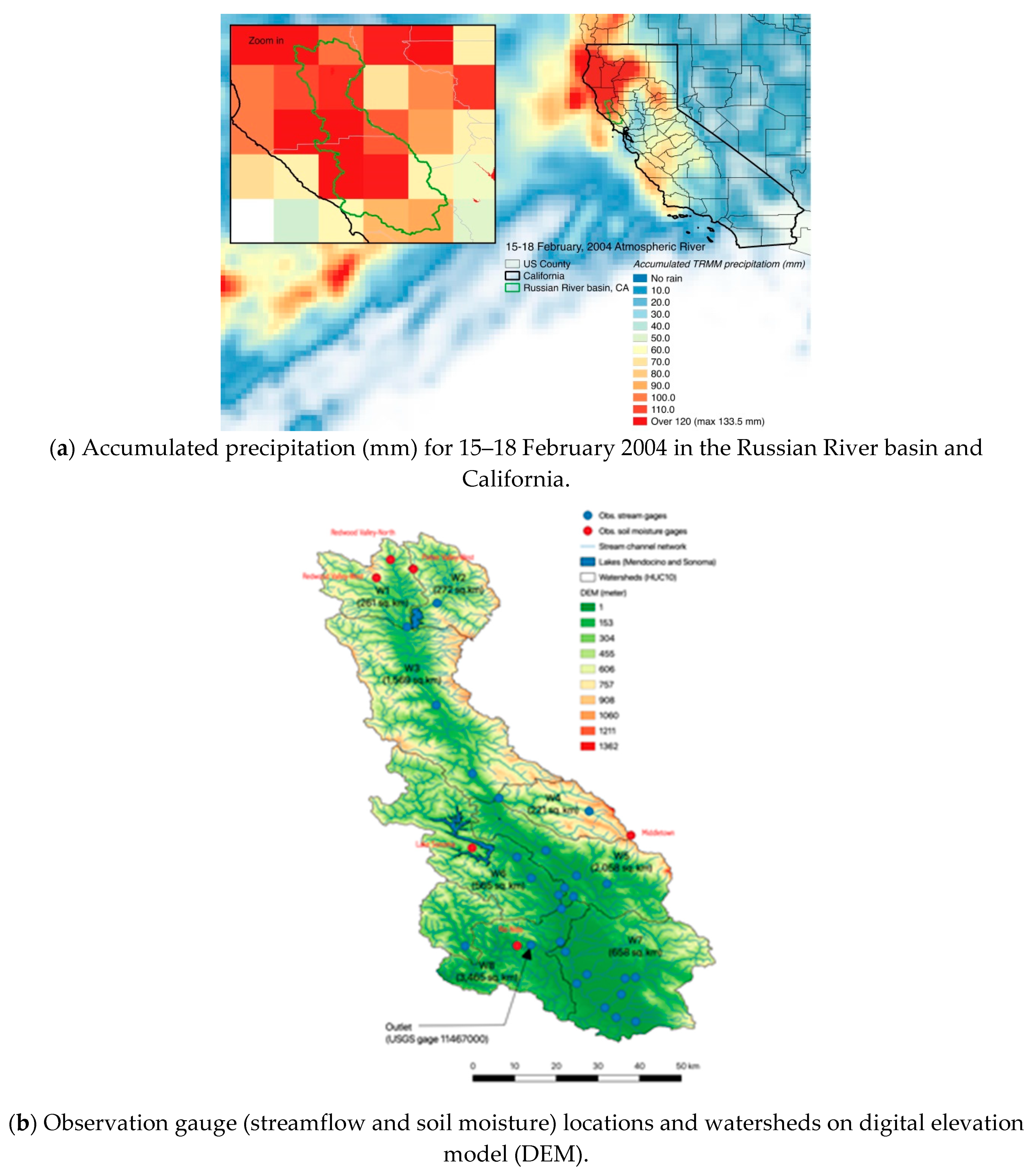
2.4.1. Study Area
2.4.2. Observation Data
3. Results
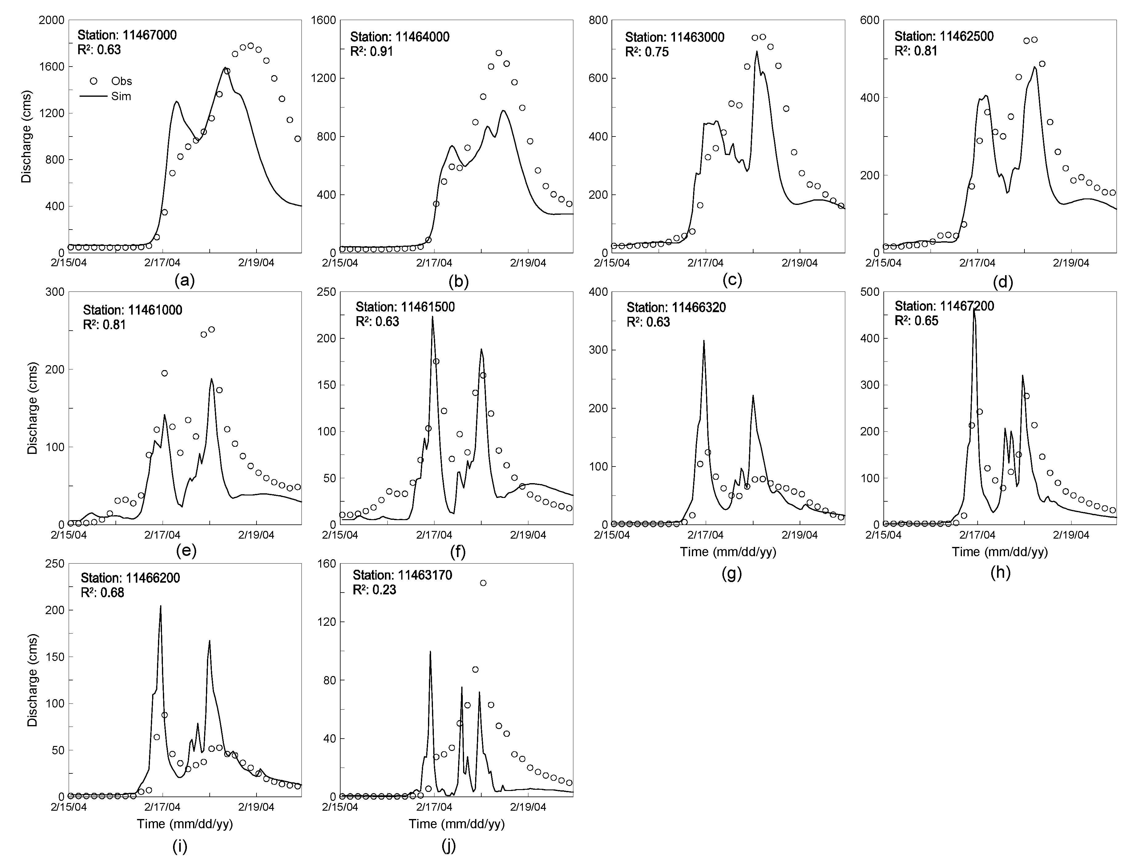
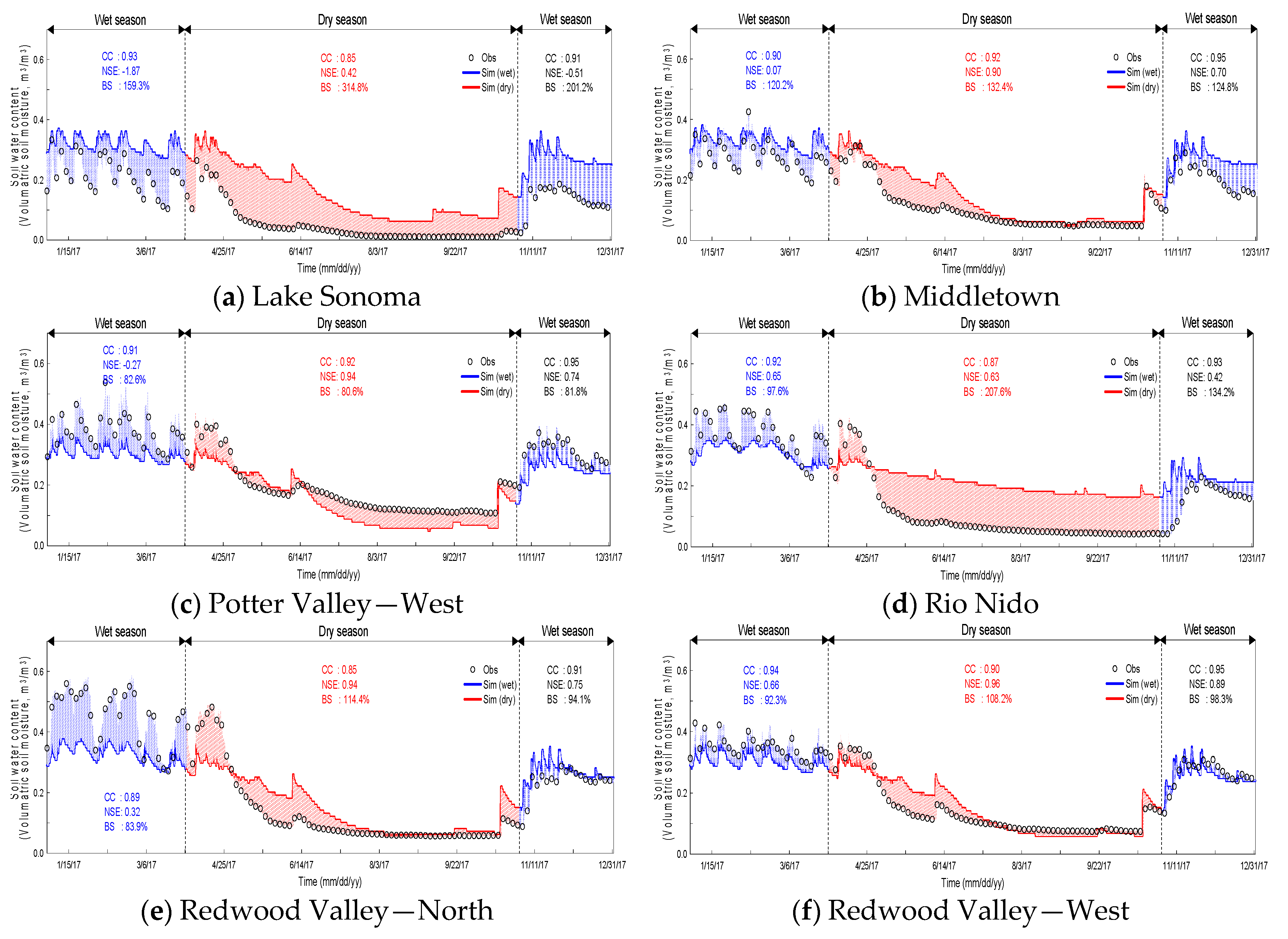
3.1. Model Verification
3.2. Hydrological Impacts of the Atmospheric River
3.2.1. Overview
3.2.2. Soil Flux
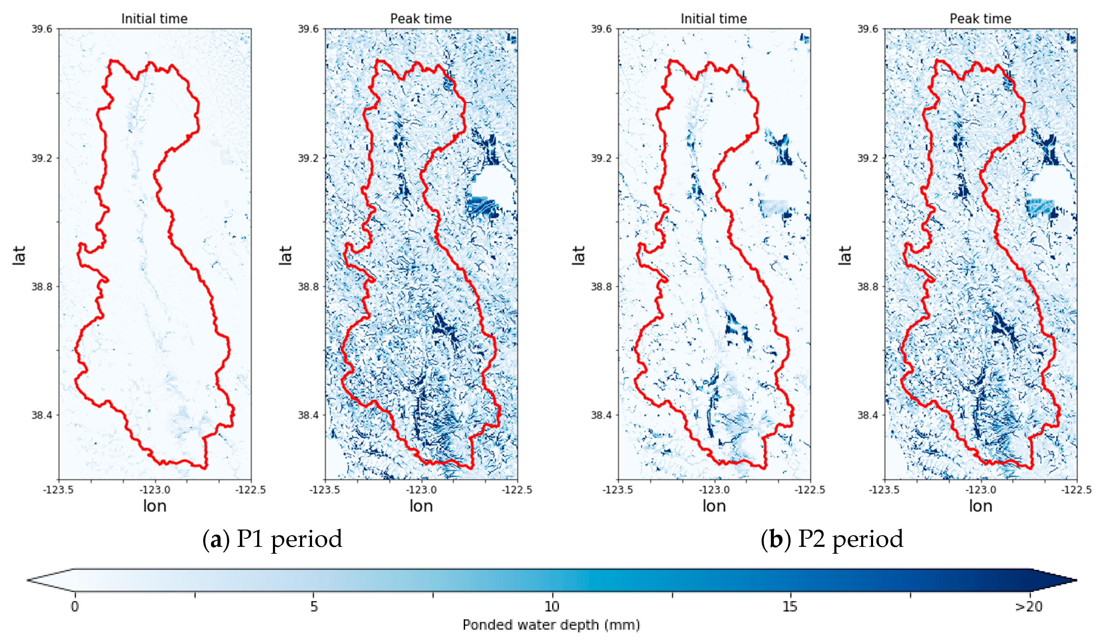
3.2.3. Surface Flow
4. Summary and Conclusions
Author Contributions
Funding
Acknowledgments
Conflicts of Interest
References
- Zhu, Y.; Newell, R.E. Atmospheric rivers and bombs. Geophys. Res. Lett. 1994, 21, 1999–2002. [Google Scholar] [CrossRef]
- Zhu, Y.; Newell, R.E. A proposed algorithm for moisture fluxes from atmospheric rivers. Mon. Weather Rev. 1998, 126, 725–735. [Google Scholar] [CrossRef]
- Ralph, F.M.; Neiman, P.J.; Wick, G.A. Satellite and CALJET aircraft observations of atmospheric rivers over the eastern North Pacific Ocean during the winter of 1997/98. Mon. Weather Rev. 2004, 132, 1721–1745. [Google Scholar] [CrossRef]
- Gimeno, L.; Nieto, R.; Vázquez, M.; Lavers, D.A. Atmospheric rivers: A mini-review. Front. Earth Sci. 2014, 2, 2. [Google Scholar] [CrossRef]
- Ralph, F.M.; Neiman, P.J.; Wick, G.A.; Gutman, S.I.; Dettinger, M.D.; Cayan, D.R.; White, A.B. Flooding on California’s Russian River: Role of atmospheric rivers. Geophys. Res. Lett. 2006, 33. [Google Scholar] [CrossRef]
- Neiman, P.J.; Schick, L.J.; Ralph, F.M.; Hughes, M.; Wick, G.A. Flooding in western Washington: The connection to atmospheric rivers. J. Hydrometeorol. 2011, 12, 1337–1358. [Google Scholar] [CrossRef]
- Hu, H.; Dominguez, F.; Wang, Z.; Lavers, D.A.; Zhang, G.; Ralph, F.M. Linking atmospheric river hydrological impacts on the US West Coast to Rossby wave breaking. J. Clim. 2017, 30, 3381–3399. [Google Scholar] [CrossRef]
- Stohl, A.; Forster, C.; Sodemann, H. Remote sources of water vapor forming precipitation on the Norwegian west coast at 60 N–a tale of hurricanes and an atmospheric river. J. Geophys. Res. Atmos. 2008, 113. [Google Scholar] [CrossRef]
- Lavers, D.A.; Villarini, G. The nexus between atmospheric rivers and extreme precipitation across Europe. Geophys. Res. Lett. 2013, 40, 3259–3264. [Google Scholar] [CrossRef]
- Mundhenk, B.D.; Barnes, E.A.; Maloney, E.D. All-season climatology and variability of atmospheric river frequencies over the North Pacific. J. Clim. 2016, 29, 4885–4903. [Google Scholar] [CrossRef]
- Hirota, N.; Takayabu, Y.N.; Kato, M.; Arakane, S. Roles of an atmospheric river and a cutoff low in the extreme precipitation event in Hiroshima on 19 August 2014. Mon. Weather Rev. 2016, 144, 1145–1160. [Google Scholar] [CrossRef]
- Kamae, Y.; Mei, W.; Xie, S.P. Climatological relationship between warm season atmospheric rivers and heavy rainfall over East Asia. J. Met. Soc. Jpn. Ser. II 2017, 95, 411–431. [Google Scholar] [CrossRef]
- Available online: https://www.noaa.gov (accessed on 15 April 2019).
- Demaria, E.; Dominguez, F.; Hu, H.; von Glinski, G.; Robles, M.; Skindlov, J.; Walter, J. Observed hydrologic impacts of landfalling atmospheric rivers in the Salt and Verde river basins of Arizona, United States. Water Resour. Res. 2017, 53, 10025–10042. [Google Scholar] [CrossRef]
- Espinoza, V.; Waliser, D.E.; Guan, B.; Lavers, D.A.; Ralph, F.M. Global Analysis of Climate Change Projection Effects on Atmospheric Rivers. Geophys. Res. Lett. 2018, 45, 4299–4308. [Google Scholar] [CrossRef]
- Zhang, W.; Villarini, G. Uncovering the role of the East Asian jet stream and heterogeneities in atmospheric rivers affecting the western United States. Proc. Natl. Acad. Sci. USA 2018, 115, 891–896. [Google Scholar] [CrossRef] [Green Version]
- Rutz, J.J.; Steenburgh, W.J.; Ralph, F.M. Climatological characteristics of atmospheric rivers and their inland infiltration over the western United States. Mon. Weather Rev. 2017, 142, 905–921. [Google Scholar] [CrossRef]
- Lamjiri, M.A.; Dettinger, M.D.; Ralph, F.M.; Guan, B. Hourly storm characteristics along the US West Coast: Role of atmospheric rivers in extreme precipitation. Geophys. Res. Lett. 2017, 44, 7020–7028. [Google Scholar] [CrossRef]
- Lavers, D.A.; Villarini, G. Atmospheric Rivers and Flooding over the Central United States. J. Clim. 2013, 26, 7829–7836. [Google Scholar] [CrossRef]
- Nayak, M.A.; Villarini, G.; Lavers, D.A. On the skill of numerical weather prediction models to forecast atmospheric rivers over the central United States. Geophys. Res. Lett. 2014, 41, 4354–4362. [Google Scholar] [CrossRef]
- Guan, B.; Waliser, D.E. Detection of atmospheric rivers: Evaluation and application of an algorithm for global studies. J. Geophys. Res. Atmos. 2015, 120, 12514–12535. [Google Scholar] [CrossRef]
- Ralph, F.M.; Coleman, T.; Neiman, P.J.; Zamora, R.J.; Dettinger, M.D. Observed impacts of duration and seasonality of atmospheric-river landfalls on soil moisture and runoff in coastal northern California. J. Hydrometeorol. 2013, 14, 443–459. [Google Scholar] [CrossRef]
- Young, A.M.; Skelly, K.T.; Cordeira, J.M. High-impact hydrologic events and atmospheric rivers in California: An investigation using the NCEI Storm Events Database. Geophys. Res. Lett. 2017, 44, 3393–3401. [Google Scholar] [CrossRef]
- Cifelli, R.; Chandrasekar, V.; Chen, H.; Johnson, L.E. High resolution radar quantitative precipitation estimation in the San Francisco Bay area: Rainfall monitoring for the urban environment. J. Met. Soc. Jpn. Ser. II 2018, 96, 141–155. [Google Scholar] [CrossRef]
- Kim, J.; Johnson, L.E.; Cifelli, R.; Coleman, T.; Herdman, L.; Martyr-Koller, R.; Finzi-Hart, J.; Erikson, L.; Barnard, P.L. San Francisco Bay Integrated Flood Forecasting Project Summary Report; NOAA Technical Memorandum PSD-317; NOAA Printing Office: Silver Spring, MD, USA, 2018. [Google Scholar]
- Available online: http://water.noaa.gov/about/nwm (accessed on 15 April 2019).
- Available online: https://ral.ucar.edu/projects/wrf_hydro/overview (accessed on 15 April 2019).
- Available online: https://ral.ucar.edu/projects/supporting-the-noaa-national-water-model (accessed on 15 April 2019).
- White, A.B.; Neiman, P.J.; Ralph, F.M.; Kingsmill, D.E.; Persson, P.O.G. Coastal orographic rainfall processesobserved by radar during the California Land-Falling Jets Experiment. J. Hydrometeorol. 2003, 4, 264–282. [Google Scholar] [CrossRef]
- Matrosov, S.Y.; Cifelli, R.; Neiman, P.J.; White, A.B. Radar rain-rate estimators and their variability due to rainfall type: An assessment based on hydrometeorology testbed data FROM the southeastern United States. J. Appl. Meteorol. Clim. 2016, 55, 1345–1358. [Google Scholar] [CrossRef]
- Willie, D.; Chen, H.; Chandrasekar, V.; Cifelli, R. Evaluation of multisensor quantitative precipitation estimation in Russian river basin. J. Hydrol. 2016, 22, 1–11. [Google Scholar] [CrossRef]
- Dettinger, M.D.; Ralph, F.M.; Das, T.; Neiman, P.J.; Cayan, D.R. Atmospheric rivers, floods and the water resources of California. Water 2011, 3, 445–478. [Google Scholar] [CrossRef]
- Kim, J.; Han, H.; Johnson, L.E.; Lim, S.; Cifelli, R. Hybrid machine learning framework for hydrological assessment. J. Hydrol. 2019, 577, 123913. [Google Scholar] [CrossRef]
- Available online: http://prism.oregonstate.edu/ (accessed on 30 April 2019).
- Kim, J.; Johnson, L.; Cifelli, R.; Choi, J.; Chandrasekar, V. Derivation of Soil Moisture Recovery Relation Using Soil Conservation Service (SCS) Curve Number Method. Water 2018, 10, 833. [Google Scholar] [CrossRef]
- Gotvald, A.J.; Barth, N.A.; Veilleux, A.G.; Parrett, C. Methods for Determining Magnitude and Frequency of Floods in California, Based on Data through Water Year 2006; Scientific Investigations Rep. 2012-5113; U.S. Dept. of the Interior, U.S. Geological Survey: Reston, VA, USA, 2012.


| Type | Size | Variable | Unit | Others |
|---|---|---|---|---|
| Grid | 1 km | Soil moisture saturation for four layers | fraction | Volumetric soil water content (m3/m3) |
| Accumulated evapotranspiration | mm | - | ||
| Snow temperature | K | - | ||
| Column-averaged snow cover fraction | fraction | - | ||
| Snow water equivalent | km/m2 | - | ||
| Snow depth | m | - | ||
| 250 m | Ponded water depth | mm | Direct runoff depth | |
| Depth to soil saturation | m | - | ||
| Point | - | Streamflow | m3/s | Discharge |
| Velocity | m/s | - | ||
| Channel inflow | m3/s | Discharge | ||
| Reservoir elevation/inflow/outflow | m and m3/s | Water level and discharge |
| Station ID (USGS) | Drainage Size (km2) | Elevation (m) | Location | Flow Type | Lake | Available Period | |
| Latitude (°) | Longitude (°) | ||||||
| 11467000 | 3465.4 | 6.2 | 38.5086 | −122.9266 | Regulated | Mendocino/Sonoma | October 1987 |
| 11464000 | 2053.9 | 23.9 | 38.6133 | −122.8352 | Regulated | Mendocino | October 1987 |
| 11463000 | 1302.8 | N/A | 38.8790 | −123.0530 | Regulated | Mendocino | October 1989 |
| 11462500 | 937.6 | 154.3 | 39.0270 | −123.1310 | Regulated | Mendocino | October 1987 |
| 11461000 | 259.0 | 185.8 | 39.1960 | −123.1940 | Natural | N/A | November 1987 |
| 11461500 | 238.8 | 244.2 | 39.2466 | −123.1291 | Natural | N/A | October 1987 |
| 11466320 | 201.0 | N/A | 38.4452 | −122.8061 | Natural | N/A | December 1998 |
| 11467200 | 162.7 | 12.4 | 38.5066 | −123.0686 | Natural | N/A | October 2003 |
| 11466200 | 147.6 | 31.0 | 38.4366 | −122.7236 | Natural | N/A | December 2001 |
| 11463170 | 33.9 | 4.1 | 38.7977 | −122.8013 | Natural | N/A | October 1987 |
| Site Name (Soil Water Content Observation) | Latitude (°) | Longitude (°) | Elevation (m) | Observation Start Date | |||
| Lake Sonoma | 38.7187 | −123.0537 | 396 | 17 December 2010 | |||
| Middletown | 38.7456 | −122.7112 | 972 | 10 December 2014 | |||
| Potter Valley—West | 39.3204 | −123.1801 | 518 | 26 May 2016 | |||
| Rio Nido | 38.5073 | −122.9565 | 39 | 2 December 2006 | |||
| Redwood Valley—North | 39.3406 | −123.2297 | 294 | 25 May2016 | |||
| Redwood Valley—West | 39.3014 | −123.2601 | 631 | 26 May 2016 | |||
| Error Indices | Acronym | Equation |
|---|---|---|
| Correlation coefficient | CC | |
| Nash–Sutcliffe efficiency | NSE | |
| Percent bias | PBIAS | |
| Bias | BS | |
| Time to peak error | TP | |
| Peak flow error | PF |
| Layer | Saturation Rate (Change in Soil Water Content in an Hour) | |
|---|---|---|
| P1 | P2 | |
| 1 | 0.0527 | 0.0125 |
| 2 | 0.0597 | 0.0103 |
| 3 | 0.0340 | 0.0129 |
| 4 | 0.0052 | 0.0164 |
| Contents | P1 (6:00 a.m. 16 February–5:00 a.m. 17 February) | P2 (6:00 a.m. 17 February–4:00 a.m. 18 February) | Total (6:00 a.m. 16 February–4:00 a.m. 18 February) |
|---|---|---|---|
| Total precipitation (mm) (%) | 75.17 (51.45%) | 70.93 (48.55%) | 146.09 (100%) |
| Duration (h) | 24 | 23 | 47 |
| Mean precipitation (mm/h) | 3.13 | 3.08 | 3.11 |
| Max precipitation (mm/h) | 13.54 | 7.14 | 13.54 |
| Accumulated direct runoff depth (mm) (%) | 22.22 (44.14%) | 28.12 (55.86%) | 50.34 (100%) |
| Ratio of direct runoff depth to precipitation | 0.296 | 0.396 | 0.345 |
© 2019 by the authors. Licensee MDPI, Basel, Switzerland. This article is an open access article distributed under the terms and conditions of the Creative Commons Attribution (CC BY) license (http://creativecommons.org/licenses/by/4.0/).
Share and Cite
Han, H.; Kim, J.; Chandrasekar, V.; Choi, J.; Lim, S. Modeling Streamflow Enhanced by Precipitation from Atmospheric River Using the NOAA National Water Model: A Case Study of the Russian River Basin for February 2004. Atmosphere 2019, 10, 466. https://doi.org/10.3390/atmos10080466
Han H, Kim J, Chandrasekar V, Choi J, Lim S. Modeling Streamflow Enhanced by Precipitation from Atmospheric River Using the NOAA National Water Model: A Case Study of the Russian River Basin for February 2004. Atmosphere. 2019; 10(8):466. https://doi.org/10.3390/atmos10080466
Chicago/Turabian StyleHan, Heechan, Jungho Kim, V. Chandrasekar, Jeongho Choi, and Sanghun Lim. 2019. "Modeling Streamflow Enhanced by Precipitation from Atmospheric River Using the NOAA National Water Model: A Case Study of the Russian River Basin for February 2004" Atmosphere 10, no. 8: 466. https://doi.org/10.3390/atmos10080466
APA StyleHan, H., Kim, J., Chandrasekar, V., Choi, J., & Lim, S. (2019). Modeling Streamflow Enhanced by Precipitation from Atmospheric River Using the NOAA National Water Model: A Case Study of the Russian River Basin for February 2004. Atmosphere, 10(8), 466. https://doi.org/10.3390/atmos10080466