The Hydrometeorology Testbed–West Legacy Observing Network: Supporting Research to Applications for Atmospheric Rivers and Beyond


National Oceanographic and Atmospheric Administration, Earth System Research Laboratory, Physical Sciences Division, Boulder, CO 80305, USA
*
Author to whom correspondence should be addressed.
Atmosphere 2019, 10(9), 533; https://doi.org/10.3390/atmos10090533
Submission received: 8 August 2019
/
Revised: 23 August 2019
/
Accepted: 24 August 2019
/
Published: 10 September 2019
(This article belongs to the Special Issue Atmospheric Rivers)
Abstract
:An observing network has been established along the United States west coast that provides up to 20 years of observations to support early warning, preparedness and studies of atmospheric rivers (ARs). The Hydrometeorology Testbed–West Legacy Observing Network, a suite of upper air and surface observing instruments, is now an official National Oceanic and Atmospheric Administration (NOAA) observing system with real-time data access provided via publicly available websites. This regional network of wind profiling radars and co-located instruments also provides observations of boundary layer processes such as complex-terrain flows that are not well depicted in the current operational rawindsonde and radar networks, satellites, or in high-resolution models. Furthermore, wind profiling radars have been deployed ephemerally for projects or campaigns in other areas, some with long records of observations. Current research uses of the observing system data are described as well as experimental products and services being transitioned from research to operations and applications. We then explore other ways in which this network and data library provide valuable resources for the community beyond ARs, including evaluation of high-resolution numerical weather prediction models and diagnosis of systematic model errors. Other applications include studies of gap flows and other terrain-influenced processes, snow level, air quality, winds for renewable energy and the predictability of cloudiness for solar energy industry.
1. Introduction
The Hydrometeorology Testbed–West Legacy Observing Network (HMT–West LON) has been successful in providing situational awareness for heavy rainfall events, and is used by the California Dept of Water Resources (CA-DWR) and west coast offices of NOAA including National Weather Service (NWS) Weather Forecast Offices (WFOs) and River Forecast Centers (RFCs). Now an official NOAA observing system, the HMT–West LON (hereafter the hydromet network or simply network) and its Atmospheric River Observatories (AROs) also provide up to 20 years of observations of key meteorological phenomena for process studies and the development of forecast evaluation, decision support, and forecaster tools, all resulting from advances in observing high impact extreme events. The system is a legacy project of the NOAA Hydrometeorology Testbed [1] which began in 2004 as the first of a series of demonstration projects in different geographical regions to enhance the understanding of region-specific processes related to precipitation, in order to extend prediction lead time [2].
Improved forecasting of ARs is crucial to safety of life and property on the west coast because they can result in flooding damage (e.g., [3,4]). For example, two successive ARs in February of 2017 resulted in the evacuation of 188,000 people, and the cost of emergency response and repairs to Oroville Dam was estimated at over $1 billion [5]. ARs are also beneficial for snowpack and water supply, providing 25–50% of all the precipitation that occurs in California, Oregon, and Washington [6], and for a large fraction of the snow water equivalent accumulated in the Sierra Nevada mountains [7]. Thus, monitoring and improved prediction can contribute to improved management of water resources, anticipating high or low river flows for water management, and freshwater inflows for marine and coastal resources.
This network is a product of a larger NOAA capability for developing and deploying advanced observing systems. Various vertical profiling radars have different optimal operations and capabilities) that can be used to complement each other and other observing networks like the NEXRAD system. These systems include the 915-MHz wind profiling (WP) radar [8], S-band precipitation profiling radar (S-PROF; [9]), snow-level radars developed from S-band frequency-modulated continuous wave (FM-CW) technology [10], and the W-band cloud profiling radars [11]. This observing capability also requires skilled engineers and technicians who develop, deploy, operate and maintain the radars, and scientists who have the knowledge to design instrumentation to address the needs of a particular science question or research project. In addition to the HMT–West Network deployed to study ARs, NOAA has deployed WP radars and co-located instruments to support research on wind energy on the Great Plains [12] and in the Pacific Northwest [13,14], hurricanes and extreme precipitation research in the Southeast U.S. [15,16], and process research in the equatorial Pacific (e.g., [17] and the Arctic (e.g., [18,19,20,21]. Deployments at over 200 stations provide a wealth of archived observations that might be exploited for other research, which is maintained and publicly available through the PSD profiler network data and image library (hereafter, the profiler library, https://www.esrl.noaa.gov/psd/data/obs/datadisplay/).
The research uses of the current network are briefly reviewed as well as examples of results transitioned from research to operations and applications. We then explore ways in which this network, its capabilities, and archived WP data library can be a valuable resource for research on other topics and areas, and find additional opportunities to apply this capability to a range of topics beyond ARs.
2. The HMT–West Legacy Observing Network
The hydromet network is an advanced observing system for high impact extreme events. The current network is a legacy of the NOAA Hydromet Testbed West Program that was funded to study ARs and related phenomena, such as the role of coastal orography in enhancing precipitation [1]. The original network also responded to the need for short term, operational weather prediction of atmospheric rivers to mitigate flood risks and to provide coastal observations [1,22,23]. An additional motivation was to understand how changes in climate could impact the frequency, intensity and other characteristics of extreme precipitation and flooding along the U.S. West Coast. The key scientific and technical advances that led to this network are described in [23,24]).
The current network (Figure 1) leverages observations made by the CaDWR, Scripps Institution of Oceanography, and UNAVCO. NOAA/PSD manages the data and operates some of the instruments under funding from the CA-DWR under a memorandum of understanding (MOU) with NOAA. The instruments include nine AROs; ten snow-level radars to measure the area of a basin that is exposed to rain versus snow; fifty-two global positioning system (GPS) receivers to observe column-integrated water vapor concentration to monitor the inland penetration of atmospheric rivers; and forty soil moisture instruments, because antecedent conditions in the basin can determine how much water from a storm can be absorbed by the ground. In addition to four coastal ARO stations, installed in California between Spring 2011 and Fall 2016, three stations in Oregon and Washington have been installed with funding from the U.S. Department of Energy. Two additional AROs with 915-MHz WP radars were installed after the Oroville Dam flooding in 2017, at the eastern end of the San Francisco Bay Delta (Twitchell Island) and near Oroville, CA. Table 1 provides measurements and instrumentation at network sites.
The network’s radars and associated instruments are suited for research on atmospheric rivers, but also for research on the boundary layer and other topics that require high temporal and spatial resolution wind data, such as terrain-influenced mesoscale flows that affect sensible weather [26,27], turbulence [28] and for intercomparison with other measurement techniques (e.g., [29]. WP radars work by emitting pulses of electromagnetic energy that are backscattered by atmospheric turbulence and the presence of precipitation (hydrometeors), e.g., [30,31]. The wavelength of the radar determines how sensitive each radar is to different types of precipitation or in clear air. By transmitting pulses of electromagnetic radiation vertically and in at least two slightly off-vertical directions, three-dimensional vector winds can be resolved. The 915-MHz radars are slightly more sensitive to precipitation than the 449s, and can make measurements of the three-dimensional wind field with precipitation present. The 449s can distinguish backscattering in both clear air and hydrometeors, and thus can make observations of winds and vertical motion in clear air and sometimes in precipitation. The 449-MHz radars have been used successfully in the low humidity conditions common in the Arctic and at the South Pole. In contrast, the NWS operational precipitation scanning radar systems (WSR88D Dual Polarization radars) that operate at S-band have some clear-air capability but generally require hydrometeors to distinguish a signal. The 449-MHz radars can take vertical observations as low as ~180 m and up to ~10 km, depending on atmospheric conditions. Furthermore, they can take higher temporal resolution vertical measurements than is often feasible and economical for other systems, such as rawindsondes, which generally are launched twice a day, and become expensive as the number increases.
3. Value for the Research Community
Observing networks and field campaigns provide the data to investigate the coupled behavior of the atmosphere interacting with the land, ocean and cryosphere. In addition to situational awareness, the hydromet network was designed to support research on West Coast winter storms and atmospheric rivers, and to improve scientific understanding of these phenomena. Rodgers [32] described some of the research uses of the then-new boundary layer profiler. The need for specific observations and the expansion of the network over time, was informed by the understanding that ARs play a significant role in creating heavy precipitation that can lead to flooding with significant impacts [3,4,33,34,35]. This network and ephemeral deployments are capabilities that support a wide range of research in NOAA and the external community, including process studies, model performance studies, and research beyond ARs in other regions or topics. This understanding is then used to develop or enhance forecasts, and to develop forecaster and decision support tools, including forecast verification tools.
3.1. Develop and Operate Observing Instrumentation
The hydromet network is the result of the PSD capability to develop instruments, and design and execute field studies, including a suite of radars and related observing equipment. PSD also maintains the field sites and data communications infrastructure. WP radars have also been deployed with co-located instruments at over 200 sites in and beyond the U.S. These ephemeral deployments, often associated with field campaigns, last from a few weeks up to 10 years at some sites (Table 2). In addition to HMT–West [1], in recent years this function has included support for field programs, including: HMT–South East [15,16], which studied heavy precipitation and flooding; the Wind Forecast Improvement Projects (WFIP, Northern Great Plains and Texas; [12], and the Second WFIP in Washington and Oregon (WFIP2, [12,13], both funded by the Department of Energy; air quality studies in Texas [36] and New England [27]. Wind profilers have been deployed in the Arctic for studies of cloud microphysics in particular [20,21,37,38], and will be deployed as part of the MOSAIC field campaign in 2019–2020. Deployments were made ephemerally on cruises in the equatorial Pacific [17], and for up to 10 years on islands in the Trans-Pacific Network [39,40]. PSD engineers have developed several other systems including a portable, relatively low-cost snow level radar [10] (see Section 3.6.2).
3.2. Serving the Data and Value-Added Products
Systems to serve the data and value-added products support research as well as monitoring. This function involves the collection, on-line processing, data quality control, and dissemination of network and profiler deployment data to enhance research and NWS operations. Recent research has also addressed the accuracy, intercomparison, calibration, and quality control of instruments and data [27,41,42,43]; ways to process wind profiler signals to access additional variables [26] (Bianco et al., 2013); and post-deployment radar calibration [44]. Evaluation of the raw data and post-processing has provided information on additional variables, e.g., snow-level [10,41], and turbulence.
Data is provided in several ways to serve different types of users. The PSD Atmospheric River Portal is aimed at California early warning and water management users (https://www.esrl.noaa.gov/psd/arportal). This site brings together hydromet network observations, satellite water vapor and Special Sensor Microwave Imager (SSM/I) data, with tools and model forecasts such as the integrated water vapor (IWV) tool, the probabilistic landfall tool, NWS Weather Prediction Center quantitative precipitation forecasts (QPF) and Global Forecast System (GFS) forecasts. Providing access to this information from a single site assists its use by the community interested in ARs, including forecasters and emergency managers. The hydromet network data is also provided to a broader operational community via the NOAA web services portal, the Meteorological Assimilation Data Ingest System (MADIS), which collects, integrates, quality controls, and distributes observations from NOAA and non-NOAA organizations. To better infuse experimental research products into NWS forecast operations, a capability has been developed to display the data and information products in the Advanced Weather Interactive Processing System (AWIPS2) meteorological display and analysis package environment. West Coast NWS offices that utilize this data in situational awareness and forecasting include the WFOs and the Northwest and California-Nevada River Forecast Centers, as well at the NWS Western Region (WR) Science Technology Infusion Division (STID). The data is also available through CaDWR’s California Data.
Exchange Center (http://cdec.water.ca.gov). The WVFT (see Section 3.6.1) provides operational access to data as well as being a forecast verification tool for the NWS Environmental Modeling Center’s High Resolution Rapid Refresh (HRRR) and Rapid Update Cycle (RAP) numerical weather prediction models. The WVFT also allows users to compare observations with experimental versions of these models as they evolve at the NOAA Global Systems Division.
Data from previous WP deployments is archived and provided via the PSD profiler network data and image library. This profiler library provides data and metadata on the hydromet network as well as the over 200 other profiler deployments (e.g., Table 2). These archived datasets provide an opportunity for the analysis of meteorological phenomena across seasons and multiple years, often providing multiple cases of a particular phenomenon.
3.3. Research on Process Understanding
The hydromet network data is used to advance process understanding of mesoscale flows in complex terrain, orographic precipitation, and other dynamical and thermodynamic mesoscale features and phenomena. Spatiotemporal analyses of mesoscale flows forced and/or modulated by complex terrain has documented the effects of ARs on sensible weather (e.g., sea-breeze effects on energy consumption and air quality, land-breeze effects on fire weather, effects of moisture flux in landfalling storms on orographic precipitation) [45], and the observed impacts of ARs on soil moisture and runoff [46]. Research on integrated water vapor (IWV) showed the threshold of IWV needed to produce extreme rainfall in the coastal mountains [47], now used in a water vapor flux tool, developed for the operational detection of ARs (see Section 3.6.1). White et al. [27] showed that a rise of 600 m in snow level (the level in the atmosphere at which precipitation freezes) could triple the peak runoff from a modest storm; this led to the development of a snow level tool (see Section 3.6.2). Hatchett and co-authors subsequently documented a trend in snow level in the decade ending in 2017 [48].
Observations of mesoscale flow direction have been used to study the inland transport of moisture through important coastal and inland terrain gaps [14,25,49], and to study processes that influence moisture fluxes and precipitation in and through Oregon’s Columbia River Gorge [14,50]. As part of CalWater-2015, these observations were used in research on baroclinically induced low-level jets (depth and strength) in landfalling storms and to improve understanding of the impact of ARs on orographic precipitation enhancement along the West Coast [25,45,51,52,53]. Completed and ongoing process studies have addressed a number of topics with implications beyond ARs and West Coast winter storms including the kinematic and thermodynamic structure of jets and ARs [54], studies of quantitative precipitation estimation [43,55,56,57] and in microphysical regime studies [54]. The observations have been used to study long range transport of aerosols and the impacts of aerosols on precipitation [58,59,60], and transport of pollutants [61] in the western U.S. Reanalysis data, including these observations, were used to show that duration and intensity of precipitation are related to the structure and evolution of warm fronts and polar cold fronts in landfalling storms [62].
3.4. Research on Model Performance and Improvement
These observations support studies of model verification and validation, the impact of observations on model performance, and parameterization, which can ultimately lead to improvements in models and services. Some examples of current research in these areas include studies of the impact of instrumentation or data assimilation on model skill, as in the impact of observations on the skill of numerical weather prediction models at forecasting wind events and wind speeds [63,64]; model verification/validation, including parameterization and algorithms [65,66,67,68]; how model improvements impact skill of wind forecasts [41,69]; and evaluation of microphysical algorithms in the Advanced Research Weather and Research Forecast Model [70]. Observations have also been used in assessing model skill in forecasting ARs during CalWater-2015 [51], and in wind speeds for wind turbines [64]. Wind and precipitation profiling radars deployed in Mexico have been used to study the North American summer monsoon [71] and GPS IWV measurements have been used by forecasters to study monsoon impacts in Southern California [72].
3.5. Research Beyond ARs
3.5.1. Wind Energy Studies
The WFIP2 field campaign used the AROs in Washington and Oregon, as well as 915-MHz radars and other instrumentation, to improve the accuracy of numerical weather prediction (NWP) model forecasts of wind speed in complex terrain for wind energy applications [13,41,65,69]. A large suite of instrumentation was deployed in the Pacific Northwest [14], including eight 915-MHz WP radars and radio acoustic sounding systems (RASS) deployed in complex terrain with many wind farms and large wind power production, and three existing coastal ARO 449-MHz radars. Observations from the Washington and Oregon AROs have been used to study the effects of marine-layer-depth behavior on sea-breeze strength and inland penetration for wind-farm operations [41]; to improve the understanding of processes that influence moisture fluxes and precipitation in and through Oregon’s Columbia River Gorge ([13,26,73,74]; to understand mountain waves [75], understanding cold pool events [68,76] and model development for wind forecasting [66,69]. The first WFIP used 915-MHz radars in its suite of instrumentation (Table 2), and found that the additional observations had a positive impact on numerical weather prediction skill [63].
3.5.2. Arctic Processes
A 449-MHz WP radar, like those at network AROs, has been deployed on a ship for PSD Arctic process studies to develop predictive understanding of Arctic processes including clouds [18,19,20,21] and sea ice [37,77]. This ongoing research supports NOAA’s mission to provide accurate and timely sea-ice forecasts, and develop a coupled ocean-atmosphere sea ice model for operational sea ice forecasting. As part of the cross-agency Earth System Prediction Capability [78], this research is testing the hypothesis that atmospheric processes drive changes in sea-ice retreat in summer and its advance in autumn in the marginal ice zone, and that these processes either directly impact the sea-ice or do so indirectly through local oceanographic processes. It is further hypothesized that uncertainties in how these atmospheric processes and associated structures or fluxes are represented in numerical models cause significant errors in forecasts of Arctic sea-ice, weather, and climate, including in model-based forcing “data” such as reanalyses. Both the research and future operational forecasting will require ongoing observations and monitoring of winds in the Arctic. The 449-MHz radars are necessary because of their capability to make observations in low moisture conditions in the Arctic and at higher temporal resolution (about 2x/hour) at which winds are thought to influence the development and expansion of sea ice leads and extent, and at lower cost than other observations, such as rawindsondes.
3.5.3. Air Quality and Dispersion Studies
WP radar observations have been used for studies to develop predictive understanding wind-related air quality [61,79,80,81], fire weather [82] (NOAA/ESRL Physical Sciences Division, 2007), methane [79,83] and NOx transportation and dispersion [80]. Boundary-layer wind profiling networks were installed to address the transport, vertical mixing, and dispersion of air pollution for major air quality related field campaigns in Alabama [84], California [85,86], Colorado [87,88], New England [89], Tennessee ([90], and Texas [36]. Many of these were ephemeral deployments of weeks to months, with data still available in the profiler library.
3.5.4. Southeastern U.S. (SEUS) Flooding and Hurricanes
A 16-month field deployment in North Carolina focused on extreme precipitation processes and forecast challenges in the SEUS, with a goal of better understanding the forcings for flooding [16]. Two 449-MHz radars were deployed as well as related observations (Table 2). These observations were used to compare ARs in the SE and along the West Coast [15], the characteristics of extreme precipitation events in the southeast [55] and how well they verify in the NCEP Global Ensemble Forecasting System [72].
3.6. Research to Operations and Applications
Research findings have been developed into tools, experimental products, and services that are being transitioned through stages into operations (e.g., development, demonstration, application, operations) or applications alongside the formal NWS transition process. Four examples below show how these observing capabilities, data provision, and process studies are yielding model improvements, or new applications, including several new forecaster tools developed in collaboration with NWS offices.
3.6.1. The Water Vapor Flux Tool (WVFT)
A web-based decision and forecaster support tool for water vapor flux and related variables has been developed to provide access to west coast data for situational awareness by the CaDWR, as well as research and NOAA operations [22,67,91]. This forecast tool (Figure 2) provides hourly-averaged freezing level, wind profiles, upslope flow, IWV, and IWV flux. The tool displays 36 h of observed and modeled values of these quantities as well as 12 h of forecasts, and the resulting precipitation. The tool was originally developed as part of the NOAA Hydromet Testbed, with partners from NOAA Global Systems Division and the NWS San Francisco/Bay Area Weather Forecast Office; the partners continue to provide the tool in the western U.S. as a legacy product of that Testbed. The tool now has been implemented since 2008 at the ongoing ARO stations, and was implemented for the HMT-Southeast stations in Florida, Mississippi, and North Carolina in 2014–2015.
The WVFT also serves as a verification tool for the NOAA High-Resolution Rapid Refresh (HRRR) and Rapid Refresh (RAP) numerical weather prediction (NWP) models, assisting in forecasting heavy precipitation events [67,91]. Forecasters can use the WVFT display to monitor the atmospheric forcings associated with ARs and to evaluate the performance of a weather forecast models’ prediction of those forcings. Horizontal winds from hourly updated HRRR analyses are retrieved to compare with profiler winds; comparison plots and difference statistics are generated every hour. Darby and co-authors [67] used HMT observations to verify forecasts of the two models for a winter study period. They found that both models did well in forecasting IWV at all AROs and winds in an elevated layer at most AROs, implying that forecasted advection of moisture to the stations was adequate, excluding the larger observed values at some AROs. However, at most stations and most hourly precipitation rates, the HRRR underpredicted precipitation, including the three stations that received the most precipitation over the study period (FKS, AST, and CZC) (Figure 2 in [67]). At several stations the RAP performed better at smaller (<1.27 mm h−1) precipitation rates, but underpredicted precipitation rates >2 mm h−1. These observation-based findings are useful as a diagnosis of models and may inform future model improvements.
Figure 2 shows the orographic enhancement in a February 2019 storm. Precipitation inland over the storm period was over 15” in the mountain catchments feeding the Russian River, which subsequently flooded [92]. The lower panel shows that the precipitation at Cazadero was about three times that at the coastal station at Bodega Bay, in a 36-h period (15.28 in vs. 4.68 in). The snow level was well forecasted 3 h in advance by the RAP (top panel). Snow level is an important indicator of whether precipitation falls as rain or snow at a particular elevation, a potential indicator of near term flood risk.
3.6.2. Snow Level Radar and Forecasting
The altitude at which snow transitions to rain, also known as the snow level, is important for determining how much of a river basin is exposed to rain versus snow, and ultimately the flood risk. For example, White and co-authors [27] demonstrated that a rise of 600 m in snow level could triple the peak runoff from a modest storm. Recognizing this importance, a specialized radar has been developed for detecting the snow level in precipitation [10] using an automated snow-level detection algorithm [27]. Ten of these radars have now been deployed in California (https://www.esrl.noaa.gov/psd/arportal/observatories). These observations have been used to evaluate NWS snow level forecasts to diagnose significant errors in forecasts from the California-Nevada River Forecast Center [93] and the Northwest River Forecast Center [94,95]. For the wettest storms caused by atmospheric rivers—the ones with high risk for flooding—the forecasts were low by several hundred meters, indicating a bias in the forecast model. Matrosov and co-authors [96] used this radar to evaluate WSR-88D estimates of snow level.
Subsequently, a new online, hourly-updated, snow-level forecast verification tool has been developed that compares observed snow levels with snow levels predicted by the HRRR numerical weather prediction model. This tool was developed in collaboration with the NWS California-Nevada River Forecast Center (CNRFC) and California WFOs and is now being used in their operations. Figure 3 shows the output of this tool and forecast for the period 6–10 February, 2017, during a period of heavy precipitation that eventually caused the Oroville Dam to overflow its emergency spillway on 12 February 2017 [5]. This shows how the HRRR struggled to predict the unusually high snow levels during the event. Even for the 1-year statistics (bottom scatterplots), the best fit lies on top of the 1:1 line for all forecast periods. The tool allows forecasters to use snow level radar data to evaluate how well the HRRR weather forecast model has performed over the last few days. It also allows forecasters to assess how the different initialization times compare for the current forecast, and how the forecasts have done over the past year [10]. Ongoing research is using this tool to study where and under which synoptic conditions does the HRRR struggle with accurately forecasting the snow level. A similar verification tool could be developed for other forecast models, such as the GFS, which would allow for longer lead time verification.
3.6.3. WFIP2 Observation-Model Evaluation Tool
WP observations are being used to study and document the synoptic/mesoscale setting for wind energy applications, and in validation studies of whether this setting is accurately depicted in the NWP models [65]. During WFIP2, the Washington and Oregon AROs, and 915-MHz WPs and other instrumentation deployed for the project was used to study NWP model forecasts of wind speed in complex terrain for wind energy applications. Improved parameterizations of the HRRR model were tested to measure the impact on the wind forecasts in the turbine rotor layer (50–200 m AGL), where wind turbines harvest wind energy. This data has been used to evaluate the impact of the observations on NWP forecasts (HRRR, RAP) [50,69]. Using the 915-MHz observations, Wilczak and others [50,65] showed large improvements in mean absolute error (MAE) for most of the hours in the diurnal cycle, especially in fall and winter, as well as improvements in temperature in the 3 km HRRR and a special 750 m HRRR-nest. They found less improvement for the coastal sites, but also found, importantly, that the parameterization modifications that help over-complex terrain do not show any meaningful detrimental impacts along the flatter-terrain coastal region.
The real-time observation visualization and model evaluation web site that was constructed for daily monitoring of model forecasts during the field campaign is shown in Figure 4. This tool continues to be used for research data analysis (e.g., [41,65,68]. Model verification for a cold pool event in late January 2017 is illustrated in Figure 4. The radars and other instruments detected a cold pool case as observed at Wasco, OR. However, observed wind speeds below 900 m are very slow (upper panel) with associated cold virtual temperatures, and the HRRR model completely underestimates the layer experiencing the cold pool (middle panel), eroding it too early. As a consequence, the errors in the model are very large (>5 °C, last panel). The tool allows the user to select the observed data of interest and the model for verification.
3.6.4. Wintertime Easterly Gap Flow Tool
Another applied outcome of WFIP2 has been the forecasting capability and forecaster tool for wintertime easterly gap flow events that are important for wind energy and for weather in the Columbia River Gorge area, including the Portland Metropolitan Area. This work is based on observations from a strategically deployed 915 MHz WP radar in the Columbia River Gorge and process studies [26]. The forecaster tool (Figure 5) includes automated detection of these events [26] that can identify and quantify wintertime easterly gap flow events using profiler and surface observations (see Figure 2 in [26]). The surface observations are key for identifying precipitation hazards (rain vs. snow vs. freezing rain) for the Portland Metropolitan Area. The WFO in Portland, OR, considers this product extremely useful for situational awareness at their forecast office [26].
4. Discussion
We have described the current hydromet network on the U.S. West Coast, which was originally designed to provide observations for situational awareness, advance warning, and study of ARs. The observations from the network’s WP radars and collocated instruments are particularly suited to studies of the spatiotemporal characteristics of the complex-terrain flows along the West Coast that are not well depicted in the current operational networks or in high-resolution models. These observations enable the objective identification of terrain-influenced mesoscale flows that affect sensible weather, and serve as a basis for observational and numerical modeling regarding the synoptic and mesoscale dynamical and physical processes governing and modulating these flows.
Because the WPs have the capability to make boundary layer measurements of winds and water vapor with high vertical and temporal resolution, these observations have also been used in a number of research topics beyond ARs, and in other regions. For example, WPs have been used in the Arctic, because of the capacity of the 449-MHz WP radar in particular to make observations in low humidity/water vapor environments, and in air quality and turbulence studies where high temporal resolution is needed. These observations are publicly available as a resource for other researchers: the regional hydromet network provides up to 20 years of observations of key meteorological phenomena with real-time data, and is available on the NOAA MADIS system and at the California Data Exchange Center. Data from over 200 other ephemeral deployments (Table 2) is archived in the PSD profiler library online. These data provide an opportunity for the analysis of meteorological phenomena across seasons and multiple years, often providing multiple cases of a particular phenomenon.
Furthermore, these observations are available as a resource to the community. This large regional network is available in real time and the substantial publicly available data archive provides opportunities for its use in research in places and for other boundary layer topics. In particular, there is an opportunity to use the network’s observations for studies to improve parameterizations of models, or understanding of particular features, such as boundary layer properties, or cloud microphysics. Ongoing or archived observations from these instruments may be used to improve models for some key places and phenomena. Having reviewed uses of this network in recent research, here we consider additional ways in which this network, the capabilities of its instruments, and archived data from other WP deployments might provide value to the community for boundary layer research. The following kinds of studies might take advantage of this existing capabilities beyond ARs.
4.1. Evaluate if Observations Improve Forecasts for Particular Events
Data denial experiments could evaluate if assimilating observations from the network or other sites would change the forecast by GFS or other forecast models. White and others [5] showed that hydromet network observations provided key information that might have improved the forecast of heavy prolonged rains at Oroville Dam in 2017, in which GFS missed the duration of the stalled front and prolonged atmospheric river conditions in the Feather River Basin. Studies could be done of other high-impact extreme weather events. Such studies might be done for other high impact events to determine the utility of new observations.
4.2. Validation of Reanalyses or Reforecast Datasets
Validation data is often lacking for reanalyses products, especially in areas where there are few observations, as on the U.S. west coast. The hydromet network, and profiler library data from other WP deployments could provide data for this purpose, similar to that described by Wang and coauthors [97], in particular, the AROs that are right on the coast, or other deployments in areas with sparse observations.
4.3. Diagnose Models for Some Key Phenomena and Places
The network and archive provide data for studying other regionally important phenomena, beyond ARs, for example cold pools and gap flows in the Columbia River area [73]. Archive data might be used to diagnose the latest weather models (e.g., the most recent operational GFS—Finite Volume Cubical Sphere, HRRR, or RAP models) for their performance on other regional or high impact phenomena previously observed with these instruments. These phenomena might include heavy precipitation in the southeast U.S., hurricanes and tornadoes, and inversions that lead to air quality issues.
4.4. Develop or Improve Parameterizations
Improved parameterizations of smaller scale features in models could have a significant effect on model forecast performance (e.g., [66]). These include convection, precipitation, snow level, and cloud microphysics. Bianco and Olson and their coauthors [66,98] demonstrated improvements in parameterizations to the HRRR, and now they are proposing testing these parameterizations for applicability in other meteorological contexts in the northern Great Plains at the DOE ARM site in Oklahoma (L. Bianco, personal communication). Parameterization development could be done in one meteorological regime then tested in the hydromet network region or using archived observations in the PSD data library. Tests could be done in other areas using the archived data.
4.5. Characterization of Boundary Layer Processes
Models might be improved with better characterization of the boundary layer using surface flux measurements to constrain models, and process studies of surface fluxes to improve parameterizations. Soil moisture sensors are co-located with WP radars at some network sites, but would need to be co-located in more stations. Co-located microwave radiometers might be used to provide vertical gradient of moisture.
4.6. Understanding Model Bias in Temperature at the Land Surface
Process studies based on near surface observations might help disentangle the sources of these known model biases (e.g., [99]), which are due to physical processes not being well represented, mis-specification of vertical mixing, or problems in forecast of solar radiation due to lack of skill in the forecast of cloudiness. This lack of skill then impacts the utility of cloudiness forecasts for solar energy.
4.7. Closing Budgets of Dynamical and Thermodynamical Properties
Understanding small scale variability improves stochastic parameterizations and thus the skill of GFS forecasts [97]. The WFIP2 radars or archived data from previous deployments of multiple WP radars may be in appropriate configuration or spacing for these budgets, or for resolving potential vorticity and vorticity gradient terms. The line of coastal ARO stations might provide opportunities to study gradients and budgets on a larger scale. Simultaneity of the observations, which could be coordinated among sites, is crucial for these studies.
4.8. Understanding Cloud Properties
As discussed by Solomon and coauthors [100], the dynamics of the cloud system are important for energy balance in the Arctic, but also other places. The 449-MHz WPs could provide observations for studies of cloud properties in the Arctic and phase partitioning of liquid and ice in clouds, including size and shape of droplets. To use the WPs in this way would require further research on how phase, size and shape of droplets in clouds can be observed by WP radars or scanning radars. Understanding cloud dynamics is important for forecasting cloudiness, which is in turn important for forecasting energy demand and solar energy production.
4.9. Vertical Air Motions in the Tropics
There are first order differences in the representation of up and down air motion in the tropics [101]. The ten-years of vertical profile observations from the Pacific profilers (Table 2) provide an opportunity to diagnose and better represent these motions, which are key to precipitation, convective heating, and the formation of Rossby waves.
4.10. Understanding Arctic Winds
Arctic sea ice forecasting requires an understanding of winds on shorter time scales that result in the opening of leads and other ice features [102]. WP observations may help understand and predict the confluence of cold fronts and other features resulting in atmospheric deformation that may stress the surface ice and result in the expansion of leads and other ice features.
Capitalizing on the opportunities provided by these resources might be realized by a combination of (1) utilizing existing and PSD profiler library data from the hydromet network, (2) developing observation-based process studies that capitalize on the existing network, for new studies or proof-of-concept efforts for future field campaigns, and (3) designing and deploying new network configurations for field programs that take advantage of the capabilities that these WPs and related instruments. provide. These efforts could ultimately lead to improvements in models and forecast skill.
5. Conclusions
The Hydrometeorology Testbed–West Legacy Observing Network was designed for studying regionally important ARs and has produced a substantial knowledge base. The network has been a valuable resource for developing and improving AR forecasts, forecaster tools, and decision support tools, including forecast verification tools, which are transitioning into operational use. In turn, improved models and forecasts have applications in a wide range of sectors affected by boundary layer processes, from warnings for ARs and flooding, water resources, and solar and wind energy industries. There is an opportunity for the existing network and the instrumentation to be a valuable resource to the community for other boundary-layer research, and may provide an example and lesson for the development of future observation-based process studies and model improvement studies. Thus the network and its capabilities have the potential to contribute to science beyond ARs and beyond the west coast region.
Author Contributions
A.J.R. designed the paper outline and wrote text for all sections. A.J.R. and A.B.W. prepared figures and tables. Both authors provided concepts and text for individual paper sections.
Funding
This work received no external funding and was funded internally by the NOAA/ESRL/Physical Sciences Division.
Acknowledgments
Conflicts of Interest
The authors declare no conflict of interest.
References
- White, A.B.; Anderson, M.L.; Dettinger, M.D.; Ralph, F.M.; Hinojosa, A.; Cayan, D.R.; Hartman, R.K.; Reynolds, D.W.; Johnson, L.E.; Schneider, T.L.; et al. A Twenty-First-Century California Observing Network for Monitoring Extreme Weather Events. J. Atmos. Ocean. Tech. 2013, 30, 1585–1603. [Google Scholar] [CrossRef] [Green Version]
- Ralph, F.M.; Intrieri, J.; Andra, D.; Atlas, R.; Boukabara, S.; Bright, D.; Davidson, P.; Entwistle, B.; Gaynor, J.; Goodman, S.; et al. The Emergence of Weather-Related Test Beds Linking Research and Forecasting Operations. B Am. Meteorol. Soc. 2013, 94, 1187–1211. [Google Scholar] [CrossRef]
- Neiman, P.J.; Schick, L.J.; Ralph, F.M.; Hughes, M.; Wick, G.A. Flooding in Western Washington: The Connection to Atmospheric Rivers. J. Hydrometeorol. 2011, 12, 1337–1358. [Google Scholar] [CrossRef]
- Ralph, F.M.; Neiman, P.J.; Wick, G.A.; Gutman, S.I.; Dettinger, M.D.; Cayan, D.R.; White, A.B. Flooding on California’s Russian River: Role of atmospheric rivers. Geophys. Res. Lett. 2006, 33. [Google Scholar] [CrossRef]
- White, A.B.; Moore, B.J.; Gottas, D.J.; Neiman, P.J. Winter Storm Conditions Leading to Excessive Runoff above California’s Oroville Dam during January and February 2017. B Am. Meteorol. Soc. 2019, 100, 55–69. [Google Scholar] [CrossRef]
- Dettinger, M. Climate Change, Atmospheric Rivers, and Floods in California - A Multimodel Analysis of Storm Frequency and Magnitude Changes. J. Am. Water Resour. As. 2011, 47, 514–523. [Google Scholar] [CrossRef]
- Guan, B.; Molotch, N.P.; Waliser, D.E.; Fetzer, E.J.; Neiman, P.J. Extreme snowfall events linked to atmospheric rivers and surface air temperature via satellite measurements. Geophys. Res. Lett. 2010, 37. [Google Scholar] [CrossRef] [Green Version]
- Carter, D.A.; Gage, K.S.; Ecklund, W.L.; Angevine, W.M.; Johnston, P.E.; Riddle, A.C.; Wilson, J.; Williams, C.R. Developments in Uhf Lower Tropospheric Wired Profiling at Noaas Aeronomy Laboratory. Radio. Sci. 1995, 30, 977–1001. [Google Scholar] [CrossRef]
- White, A.B.; Jordan, J.R.; Martner, B.E.; Ralph, F.M.; Bartram, B.W. Extending the dynamic range of an S-band radar for cloud and precipitation studies. J. Atmos. Ocean. Tech. 2000, 17, 1226–1234. [Google Scholar] [CrossRef]
- Johnston, P.E.; Jordan, J.R.; White, A.B.; Carter, D.A.; Costa, D.M.; Ayers, T.E. The NOAA FM-CW Snow-Level Radar. J. Atmos. Ocean. Tech. 2017, 34, 249–267. [Google Scholar] [CrossRef]
- Moran, K.; Pezoa, S.; Fairall, C.; Williams, C.; Ayers, T.; Brewer, A.; de Szoeke, S.P.; Ghate, V. A Motion-Stabilized W-Band Radar for Shipboard Observations of Marine Boundary-Layer Clouds. Bound.-Lay. Meteorol. 2012, 143, 3–24. [Google Scholar] [CrossRef]
- Wilczak, J.; Finley, C.; Freedman, J.; Cline, J.; Bianco, L.; Olson, J.; Djalalova, I.; Sheridan, L.; Ahlstrom, M.; Manobianco, J.; et al. The Wind Forecast Improvement Project (WFIP) A Public-Private Partnership Addressing Wind Energy Forecast Needs. B Am. Meteorol. Soc. 2015, 96, 1699–1718. [Google Scholar] [CrossRef]
- Shaw, W.J.; Berg, L.K.; Cline, J.; Draxl, C.; Djalalova, I.; Grimit, E.P.; Lundquist, J.K.; Marquis, M.; McCaa, J.; Olson, J.B.; et al. The Second Wind Forecast Improvement Project (WFIP2): General Overview. B Am. Meteorol. Soc. 2019. [Google Scholar] [CrossRef]
- Wilczak, J.M.; Stoelinga, M.; Berg, L.K.; Sharp, J.; Draxl, C.; McCaffrey, K.; Banta, R.M.; Bianco, L.; Djalalova, I.; Lundquist, J.K.; et al. The Second Wind Forecast Improvement Project (WFIP2): Observational Field Campaign. B Am. Meteorol. Soc. 2019. [Google Scholar] [CrossRef]
- Mahoney, K.; Jackson, D.L.; Neiman, P.; Hughes, M.; Darby, L.; Wick, G.; White, A.; Sukovich, E.; Cifelli, R. Understanding the Role of Atmospheric Rivers in Heavy Precipitation in the Southeast United States. Mon. Weather Rev. 2016, 144, 1617–1632. [Google Scholar] [CrossRef]
- White, A.B.; Mahoney, K.M.; Cifelli, R.; King, C.W. Wind Profilers to Aid with Monitoring and Forecasting of High-Impact Weather in the Southeastern and Western United States. B Am. Meteorol. Soc. 2015, 96, 2039–2043. [Google Scholar] [CrossRef]
- Fairall, C.W.; White, A.B.; Edson, J.B.; Hare, J.E. Integrated shipboard measurements of the marine boundary layer. J. Atmos. Ocean. Tech. 1997, 14, 338–359. [Google Scholar] [CrossRef]
- Sotiropoulou, G.; Tjernstrom, M.; Sedlar, J.; Achtert, P.; Brooks, B.J.; Brooks, I.M.; Persson, P.O.G.; Prytherch, J.; Salisbury, D.J.; Shupe, M.D.; et al. Atmospheric Conditions during the Arctic Clouds in Summer Experiment (ACSE): Contrasting Open Water and Sea Ice Surfaces during Melt and Freeze-Up Seasons. J. Clim. 2016, 29, 8721–8744. [Google Scholar] [CrossRef] [Green Version]
- Persson, P.O.G.; Fairall, C.W.; Andreas, E.L.; Guest, P.S.; Perovich, D.K. Measurements near the Atmospheric Surface Flux Group tower at SHEBA: Near-surface conditions and surface energy budget. J. Geophys. Res.-Oceans 2002, 107. [Google Scholar] [CrossRef]
- Tjernström, M.; Leck, C.; Birch, C.E.; Bottenheim, J.W.; Brooks, B.J.; Brooks, I.M.; Backlin, L.; Chang, Y.W.; de Leeuw, G.; Di Liberto, L.; et al. The Arctic Summer Cloud Ocean Study (ASCOS): overview and experimental design. Atmos. Chem. Phys. 2014, 14, 2823–2869. [Google Scholar] [CrossRef] [Green Version]
- Tjernström, M.; Leck, C.; Persson, P.O.G.; Jensen, M.L.; Oncley, S.P.; Targino, A. The summertime Arctic atmosphere - Meteorological measurements during the Arctic Ocean experiment 2001. B Am. Meteorol. Soc. 2004, 85, 1305–1321. [Google Scholar] [CrossRef]
- Neiman, P.J.; White, A.B.; Ralph, F.M.; Gottas, D.J.; Gutman, S.I. A water vapour flux tool for precipitation forecasting. P I Civil. Eng.-Wat. M 2009, 162, 83–94. [Google Scholar] [CrossRef]
- White, A.B.; Ralph, F.M.; Neiman, P.J.; Gottas, D.J.; Gutman, S.I. The NOAA coastal atmospheric river observatory. In Proceedings of the 34th Conference on Radar Meteorology, Williamsburg, VA, USA, 5–9 October 2009; p. 10B.14. [Google Scholar]
- Ralph, F.M.; Dettinger, M.; White, A.; Reynolds, D.; Cayan, D.; Schneider, T.; Cifelli, R.; Redmond, K.; Anderson, M.; Gherke, F.; et al. A Vision for Future Observations for Western U.S. Extreme Precipitation and Flooding. J. Contemp. Wat. Res. Ed. 2014, 153, 16–32. [Google Scholar] [CrossRef]
- White, A.B.; Neiman, P.J.; Creamean, J.M.; Coleman, T.; Ralph, F.M.; Prather, K.A. The Impacts of California’s San Francisco Bay Area Gap on Precipitation Observed in the Sierra Nevada during HMT and CalWater. J. Hydrometeorol. 2015, 16, 1048–1069. [Google Scholar] [CrossRef]
- Neiman, P.J.; Gottas, D.J.; White, A.B.; Schneider, W.R.; Bright, D.R. A Real-Time Online Data Product that Automatically Detects Easterly Gap-Flow Events and Precipitation Type in the Columbia River Gorge. J. Atmos. Ocean. Tech. 2018, 35, 2037–2052. [Google Scholar] [CrossRef]
- White, A.B.; Gottas, D.J.; Strem, E.T.; Ralph, F.M.; Neiman, P.J. An automated brightband height detection algorithm for use with Doppler radar spectral moments. J. Atmos. Ocean. Tech. 2002, 19, 687–697. [Google Scholar] [CrossRef]
- Bianco, L.; Gottas, D.; Wilczak, J.M. Implementation of a Gabor Transform Data Quality-Control Algorithm for UHF Wind Profiling Radars. J. Atmos. Ocean. Tech. 2013, 30, 2697–2703. [Google Scholar] [CrossRef]
- Lundquist, J.K.; Wilczak, J.M.; Ashton, R.; Bianco, L.; Brewer, W.A.; Choukulkar, A.; Clifton, A.; Debnath, M.; Delgado, R.; Friedrich, K.; et al. ASSESSING STATE-OF-THE-ART CAPABILITIES FOR PROBING THE ATMOSPHERIC BOUNDARY LAYER: The XPIA Field Campaign. B Am. Meteorol. Soc. 2017, 98, 289–314. [Google Scholar] [CrossRef]
- Ecklund, W.L.; Carter, D.A.; Balsley, B.B. A UHF Wind Profiler for the Boundary Layer: Brief Description and Initial Results. J. Atmos. Ocean. Tech. 1988, 5, 432–441. [Google Scholar] [CrossRef]
- Gage, K.S.; Williams, C.R.; Ecklund, W.L. Uhf Wind Profilers—A New Tool for Diagnosing Tropical Convective Cloud Systems. B Am. Meteorol. Soc. 1994, 75, 2289–2294. [Google Scholar] [CrossRef]
- Rogers, R.R.; Ecklund, W.L.; Carter, D.A.; Gage, K.S.; Ethier, S.A. Research Applications of a Boundary-Layer Wind Profiler. B Am. Meteorol. Soc. 1993, 74, 567–580. [Google Scholar] [CrossRef] [Green Version]
- Moore, B.J.; Neiman, P.J.; Ralph, F.M.; Barthold, F.E. Physical Processes Associated with Heavy Flooding Rainfall in Nashville, Tennessee, and Vicinity during 1-2 May 2010: The Role of an Atmospheric River and Mesoscale Convective Systems. Mon. Weather Rev. 2012, 140, 358–378. [Google Scholar] [CrossRef]
- Lavers, D.A.; Allan, R.P.; Wood, E.F.; Villarini, G.; Brayshaw, D.J.; Wade, A.J. Winter floods in Britain are connected to atmospheric rivers. Geophys. Res. Lett. 2011, 38. [Google Scholar] [CrossRef] [Green Version]
- Leung, L.R.; Qian, Y. Atmospheric rivers induced heavy precipitation and flooding in the western US simulated by the WRF regional climate model. Geophys. Res. Lett. 2009, 36. [Google Scholar] [CrossRef]
- Parrish, D.D.; Allen, D.T.; Bates, T.S.; Estes, M.; Fehsenfeld, F.C.; Feingold, G.; Ferrare, R.; Hardesty, R.M.; Meagher, J.F.; Nielsen-Gammon, J.W.; et al. Overview of the Second Texas Air Quality Study (TexAQS II) and the Gulf of Mexico Atmospheric Composition and Climate Study (GoMACCS). J. Geophys. Res.-Atmos. 2009, 114, D00F13. [Google Scholar] [CrossRef]
- Persson, O.; Vihma, T. The atmosphere over sea ice. In Sea Ice, 3rd ed.; Thomas, D.N., Ed.; John Wiley & Sons, Ltd.: Hoboken, NJ, USA, 2016. [Google Scholar]
- Shupe, M.D.; Uttal, T.; Matrosov, S.Y. Arctic cloud microphysics retrievals from surface-based remote sensors at SHEBA. J. Appl. Meteorol. 2005, 44, 1544–1562. [Google Scholar] [CrossRef]
- Miller, E.R.; Riddle, A.C. TOGA COARE Integrated Sounding System Data Report—Volume IA Revised Edition, 1994. National Center for Atmospheric Research: Boulder, CO, June 1994. Available online: https://aspace.archives.ucar.edu/repositories/2/archival_objects/4672 (accessed on 27 August 2019).
- Webster, P.J.; Lukas, R. Toga Coare - the Coupled Ocean Atmosphere Response Experiment. B Am. Meteorol. Soc. 1992, 73, 1377–1416. [Google Scholar] [CrossRef]
- Bianco, L.; Friedrich, K.; Wilczak, J.M.; Hazen, D.; Wolfe, D.; Delgado, R.; Oncley, S.P.; Lundquist, J.K. Assessing the accuracy of microwave radiometers and radio acoustic sounding systems for wind energy applications. Atmos. Meas. Tech. 2017, 10, 1707–1721. [Google Scholar] [CrossRef] [Green Version]
- Cannon, F.; Ralph, F.M.; Wilson, A.M.; Lettenmaier, D.P. GPM Satellite Radar Measurements of Precipitation and Freezing Level in Atmospheric Rivers: Comparison With Ground-Based Radars and Reanalyses. J. Geophys. Res.-Atmos. 2017, 122, 12747–12764. [Google Scholar] [CrossRef]
- Cifelli, R.; Chandrasekar, V.; Chen, H.N.; Johnson, L.E. High Resolution Radar Quantitative Precipitation Estimation in the San Francisco Bay Area: Rainfall Monitoring for the Urban Environment. J. Meteorol. Soc. Jpn. 2018, 96a, 141–155. [Google Scholar] [CrossRef]
- Hartten, L.M.; Johnston, P.E.; Rodríguez Castro, V.M.; Esteban Pérez, P.S. Post-Deployment Calibration of a Tropical UHF Profiling Radar via Surface- and Satellite-Based Methods. J. Atmos. Ocean. Tech. 2019. [Google Scholar] [CrossRef]
- Neiman, P.J.; Moore, B.J.; White, A.B.; Wick, G.A.; Aikins, J.; Jackson, D.L.; Spackman, J.R.; Ralph, F.M. An Airborne and Ground-Based Study of a Long-Lived and Intense Atmospheric River with Mesoscale Frontal Waves Impacting California during CalWater-2014. Mon. Weather Rev. 2016, 144, 1115–1144. [Google Scholar] [CrossRef]
- Ralph, F.M.; Coleman, T.; Neiman, P.J.; Zamora, R.J.; Dettinger, M.D. Observed Impacts of Duration and Seasonality of Atmospheric-River Landfalls on Soil Moisture and Runoff in Coastal Northern California. J. Hydrometeorol. 2013, 14, 443–459. [Google Scholar] [CrossRef] [Green Version]
- Ralph, F.M.; Neiman, P.J.; Wick, G.A. Satellite and CALJET aircraft observations of atmospheric rivers over the eastern north pacific ocean during the winter of 1997/98. Mon. Weather Rev. 2004, 132, 1721–1745. [Google Scholar] [CrossRef]
- Hatchett, B.J.; Daudert, B.; Garner, C.B.; Oakley, N.S.; Putnam, A.E.; White, A.B. Winter Snow Level Rise in the Northern Sierra Nevada from 2008 to 2017. Water 2017, 9, 899. [Google Scholar] [CrossRef]
- Mueller, M.; Mahoney, K.; Hughes, M. High-Resolution Model-Based Investigation of Moisture Transport into the Pacific Northwest during a Strong Atmospheric River Event. In Proceedings of the 98th American Meteorological Society (AMS) Annual Meeting, Austin, TX, USA, 7–11 January 2018. [Google Scholar]
- Wilczak, J.M.; Olson, J.B.; Djalalova, I.; Bianco, L.; Berg, L.K.; Shaw, W.J.; Coulter, R.L.; Eckman, R.M.; Freedman, J.; Finley, C.; et al. Data assimilation impact of in situ and remote sensing meteorological observations on wind power forecasts during the first Wind Forecast Improvement Project (WFIP). Wind Energy 2019, 22, 932–944. [Google Scholar] [CrossRef]
- Cordeira, J.M.; Ralph, F.M.; Martin, A.; Gaggggini, N.; Spackman, J.R.; Neiman, P.J.; Rutz, J.J.; Pierce, R. Forecasting Atmospheric Rivers during CalWater 2015. B Am. Meteorol. Soc. 2017, 98, 449–459. [Google Scholar] [CrossRef]
- Fairall, C.W.; Matrosov, S.Y.; Williams, C.R.; Walsh, E.J. Estimation of Rain Rate from Airborne Doppler W-Band Radar in CalWater-2. J. Atmos. Ocean. Tech. 2018, 35, 593–608. [Google Scholar] [CrossRef]
- Ralph, F.M.; Prather, K.A.; Cayan, D.; Spackman, J.R.; DeMott, P.; Dettinger, M.; Fairall, C.; Leung, R.; Rosenfeld, D.; Rutledge, S.; et al. Calwater Field Studies Designed to Quantify the Roles of Atmospheric Rivers and Aerosols in Modulating Us West Coast Precipitation in a Changing Climate. B Am. Meteorol. Soc. 2016, 97, 1209–1228. [Google Scholar] [CrossRef]
- Kingsmill, D.E.; Neiman, P.J.; White, A.B. Microphysics Regime Impacts on the Relationship between Orographic Rain and Orographic Forcing in the Coastal Mountains of Northern California. J. Hydrometeorol. 2016, 17, 2905–2922. [Google Scholar] [CrossRef]
- Matrosov, S.Y.; Cifelli, R.; Neiman, P.J.; White, A.B. Radar Rain-Rate Estimators and Their Variability due to Rainfall Type: An Assessment Based on Hydrometeorology Testbed Data from the Southeastern United States. J. Appl. Meteorol. Clim. 2016, 55, 1345–1358. [Google Scholar] [CrossRef]
- Matrosov, S.Y.; Ralph, F.M.; Neiman, P.J.; White, A.B. Quantitative Assessment of Operational Weather Radar Rainfall Estimates over California’s Northern Sonoma County Using HMT-West Data. J. Hydrometeorol. 2014, 15, 393–410. [Google Scholar] [CrossRef]
- Willie, D.; Chen, H.N.; Chandrasekar, V.; Cifelli, R.; Campbell, C.; Reynolds, D.; Matrosov, S.; Zhang, Y. Evaluation of Multisensor Quantitative Precipitation Estimation in Russian River Basin. J. Hydrol. Eng. 2017, 22. [Google Scholar] [CrossRef]
- Creamean, J.M.; Ault, A.P.; White, A.B.; Neiman, P.J.; Ralph, F.M.; Minnis, P.; Prather, K.A. Impact of interannual variations in sources of insoluble aerosol species on orographic precipitation over California’s central Sierra Nevada. Atmos. Chem. Phys. 2015, 15, 6535–6548. [Google Scholar] [CrossRef]
- Creamean, J.M.; Suski, K.J.; Rosenfeld, D.; Cazorla, A.; DeMott, P.J.; Sullivan, R.C.; White, A.B.; Ralph, F.M.; Minnis, P.; Comstock, J.M.; et al. Dust and Biological Aerosols from the Sahara and Asia Influence Precipitation in the Western U.S. Science 2013, 339, 1572–1578. [Google Scholar] [CrossRef] [PubMed]
- Creamean, J.M.; White, A.B.; Minnis, P.; Palikonda, R.; Spangenberg, D.A.; Prather, K.A. The relationships between insoluble precipitation residues, clouds, and precipitation over California’s southern Sierra Nevada during winter storms. Atmos. Environ. 2016, 140, 298–310. [Google Scholar] [CrossRef]
- Martin, A.C.; Cornwell, G.C.; Atwood, S.A.; Moore, K.A.; Rothfuss, N.E.; Taylor, H.; DeMott, P.J.; Kreidenweis, S.M.; Petters, M.D.; Prather, K.A. Transport of pollution to a remote coastal site during gap flow from California’s interior: Impacts on aerosol composition, clouds, and radiative balance. Atmos. Chem. Phys. 2017, 17, 1491–1509. [Google Scholar] [CrossRef]
- Moore, B.J.; Mahoney, K.M.; Sukovich, E.M.; Cifelli, R.; Hamill, T.M. Climatology and Environmental Characteristics of Extreme Precipitation Events in the Southeastern United States. Mon. Weather Rev. 2015, 143, 718–741. [Google Scholar] [CrossRef]
- Akish, E.; Bianco, L.; Djalalova, I.V.; Wilczak, J.M.; Olson, J.B.; Freedman, J.; Finley, C.; Cline, J. Measuring the impact of additional instrumentation on the skill of numerical weather prediction models at forecasting wind ramp events during the first Wind Forecast Improvement Project (WFIP). Wind Energy 2019, 22, 1165–1174. [Google Scholar] [CrossRef] [Green Version]
- Djalalova, I.V.; Olson, J.; Carley, J.R.; Bianco, L.; Wilczak, J.M.; Pichugina, Y.; Banta, R.; Marquis, M.; Cline, J. The POWER Experiment: Impact of Assimilation of a Network of Coastal Wind Profiling Radars on Simulating Offshore Winds in and above the Wind Turbine Layer. Weather Forecast 2016, 31, 1071–1091. [Google Scholar] [CrossRef] [Green Version]
- Wilczak, J.; McCaffrey, K.; Djalalova, I.V.; Bianco, L.; Olson, J.B.; Kenyon, J.; Stoelinga, M.T.; Sharp, J.; Pekour, M.; Cook, D.; et al. Identification and Analysis of Forecast Model Large Error Events During WFIP2. In Proceedings of the 98th American Meteorological Society (AMS) Annual Meeting, Austin, TX, USA, 7–11 January 2018; Available online: https://ams.confex.com/ams/98Annual/webprogram/Paper332680.html (accessed on 10 September 2019).
- Bianco, L.; Djalalova, I.V.; Wilczak, J.M.; Olson, J.B.; Kenyon, J.S.; Choukulkar, A.; Berg, L.K.; Fernando, H.J.S.; Grimit, E.P.; Krishnamurthy, R.; et al. Impact of model improvements on 80-m wind speeds during the second Wind Forecast Improvement Project (WFIP2). Geosci. Model. Dev. Discuss. 2019, 2019, 1–35. [Google Scholar] [CrossRef]
- Darby, L.; White, A.B.; Gottas, D.; Coleman, T. An evaluation of integrated water vapor, wind, and precipitation forecasts using water vapor flux observations in the Western United States. Weather Forecast. 2019. in review. [Google Scholar]
- Wilczak, J.M.; McCaffrey, K.; Draxl, C.; Olson, J.B.; Stoelinga, M.T.; Berg, L.K.; Bianco, L.; Choukulkar, A.; Djalalova, I.V.; Grimit, E.P.; et al. Improved Understanding and Modeling of Key Atmospheric Phenomena during WFIP2: Cold Pools, Gap Flows, and Mountain Waves. In Proceedings of the 98th American Meteorological Society (AMS) Annual Meeting, Phoenix, AZ, USA, 6–10 January 2019; Available online: https://ams.confex.com/ams/2019Annual/meetingapp.cgi/Paper/354155 (accessed on 10 September 2019).
- Olson, J.B.; Kenyon, J.S.; Djalalova, I.; Bianco, L.; Turner, D.D.; Pichugina, Y.; Choukulkar, A.; Toy, M.D.; Brown, J.M.; Angevine, W.M.; et al. Improving Wind Energy Forecasting through Numerical Weather Prediction Model Development. B Am. Meteorol. Soc. 2019. [Google Scholar] [CrossRef]
- Jankov, I.; Bao, J.W.; Neiman, P.J.; Schultz, P.J.; Yuan, H.L.; White, A.B. Evaluation and Comparison of Microphysical Algorithms in ARW-WRF Model Simulations of Atmospheric River Events Affecting the California Coast. J. Hydrometeorol. 2009, 10, 847–870. [Google Scholar] [CrossRef]
- Williams, C.R.; White, A.B.; Gage, K.S.; Ralph, F.M. Vertical structure of precipitation and related microphysics observed by NOAA profilers and TRMM during NAME 2004. J. Clim. 2007, 20, 1693–1712. [Google Scholar] [CrossRef]
- Moore, A.W.; Small, I.J.; Gutman, S.I.; Bock, Y.; Dumas, J.L.; Fang, P.; Haase, J.S.; Jackson, M.E.; Laber, J.L. National Weather Service Forecasters Use GPS Precipitable Water Vapor for Enhanced Situational Awareness during the Southern California Summer Monsoon. B Am. Meteorol. Soc. 2015, 96, 1867–1877. [Google Scholar] [CrossRef]
- McCaffrey, K.; Bianco, L.; Djalalova, I.V.; Wilczak, J.M.; Grimit, E.P.; Sharp, J.; Leo, L.; Friedrich, K.; Bonin, T.; Choukulkar, A. Identification and Characterization of Cold Pool Events in the Columbia River Basin during WFIP2. J. Appl. Meteorol. Clim. 2019, in press. [Google Scholar]
- Pichugina, Y.L.; Banta, R.M.; Bonin, T.; Brewer, W.A.; Choukulkar, A.; McCarty, B.J.; Baidar, S.; Draxl, C.; Fernando, H.J.S.; Kenyon, J.; et al. Spatial Variability of Winds and HRRR-NCEP Model Error Statistics at Three Doppler-Lidar Sites in the Wind-Energy Generation Region of the Columbia River Basin. J. Appl. Meteorol. Clim. 2019, 58, 1633–1656. [Google Scholar] [CrossRef]
- Draxl, C.; Quon, D.; Chand, D.; Berg, L.K.; Churchfield, M.J.; Kemper, T.; Kenyon, J.; Olson, J.B.; Sharp, J. Simulated and Observed Mountain Waves and Their Implications on Wind Energy. In Proceedings of the 98th American Meteorological Society (AMS) Annual Meeting, Austin, TX USA, 7–11 January 2018; Available online: https://ams.confex.com/ams/98Annual/webprogram/Paper336065.html (accessed on 10 September 2019).
- McCaffrey, K.E.; Wilczak, J.M.; Bianco, L.; IDjalalova, I.V.; Banta, R.; Bonin, T.A.; Brewer, W.A.; Choukulkar, A.; Cook, D.; Coulter, R.L.; et al. Identification and Characterization of Cold Pool Events during WFIP2. In Proceedings of the 98th American Meteorological Society (AMS) Annual Meeting, Austin, TX, USA, 7–11 January 2018; Available online: https://ams.confex.com/ams/98Annual/webprogram/Paper331305.html (accessed on 10 September 2019).
- Lund, B.; Graber, H.C.; Persson, P.O.G.; Smith, M.; Doble, M.; Thomson, J.; Wadhams, P. Arctic Sea Ice Drift Measured by Shipboard Marine Radar. J. Geophys. Res.-Oceans 2018, 123, 4298–4321. [Google Scholar] [CrossRef]
- Carman, J.C.; Eleuterio, D.P.; Gallaudet, T.C.; Geernaert, G.L.; Harr, P.A.; Kaye, J.A.; McCarren, D.H.; McLean, C.N.; Sandgathe, S.A.; Toepfer, F.; et al. The National Earth System Prediction Capability: Coordinating the Giant. B Am. Meteorol. Soc. 2017, 98, 239–252. [Google Scholar] [CrossRef] [Green Version]
- Jeong, S.; Hsu, Y.K.; Andrews, A.E.; Bianco, L.; Vaca, P.; Wilczak, J.M.; Fischer, M.L. A multitower measurement network estimate of California’s methane emissions. J. Geophys. Res.-Atmos. 2013, 118, 11339–11351. [Google Scholar] [CrossRef]
- Jeong, S.; Newman, S.; Zhang, J.S.; Andrews, A.E.; Bianco, L.; Dlugokencky, E.; Bagley, J.; Cui, X.G.; Priest, C.; Campos-Pineda, M.; et al. Inverse Estimation of an Annual Cycle of California’s Nitrous Oxide Emissions. J. Geophys. Res.-Atmos. 2018, 123, 4758–4771. [Google Scholar] [CrossRef]
- Bao, J.W.; Michelson, S.A.; Persson, P.O.G.; Djalalova, I.V.; Wilczak, J.M. Observed and WRF-simulated low-level winds in a high-ozone episode during the Central California Ozone Study. J. Appl. Meteorol. Clim. 2008, 47, 2372–2394. [Google Scholar] [CrossRef]
- NOAA/ESRL Physical Sciences Division. Coastal Wind Profiler Technology Evaluation: An. Integrated Ocean. Observing System Project Final Report; November 2007. Available online: https://www.esrl.noaa.gov/psd/news/2007/pdf/IOOS_Final%20Report_Nov_15_2007.pdf (accessed on 27 August 2019).
- Schwietzke, S.; Petron, G.; Conley, S.; Pickering, C.; Mielke-Maday, I.; Dlugokencky, E.J.; Tans, P.P.; Vaughn, T.; Bell, C.; Zimmerle, D.; et al. Improved Mechanistic Understanding of Natural Gas Methane Emissions from Spatially Resolved Aircraft Measurements. Environ. Sci. Technol. 2017, 51, 7286–7294. [Google Scholar] [CrossRef] [PubMed] [Green Version]
- Frost, G.J.; Trainer, M.; Allwine, G.; Buhr, M.P.; Calvert, J.G.; Cantrell, C.A.; Fehsenfeld, F.C.; Goldan, P.D.; Herwehe, J.; Hubler, G.; et al. Photochemical ozone production in the rural southeastern United States during the 1990 Rural Oxidants in the Southern Environment (ROSE) program. J. Geophys. Res.-Atmos. 1998, 103, 22491–22508. [Google Scholar] [CrossRef]
- Croes, B.E.; Fujita, E.M. Overview of the 1997 Southern California Ozone Study (SCOS97-NARSTO). Atmos. Environ. 2003, 37, S3–S26. [Google Scholar] [CrossRef]
- Ryerson, T.B.; Andrews, A.E.; Angevine, W.M.; Bates, T.S.; Brock, C.A.; Cairns, B.; Cohen, R.C.; Cooper, O.R.; de Gouw, J.A.; Fehsenfeld, F.C.; et al. The 2010 California Research at the Nexus of Air Quality and Climate Change (CalNex) field study. J. Geophys. Res.-Atmos. 2013, 118, 5830–5866. [Google Scholar] [CrossRef]
- Petron, G.; Karion, A.; Sweeney, C.; Miller, B.R.; Montzka, S.A.; Frost, G.J.; Trainer, M.; Tans, P.; Andrews, A.; Kofler, J.; et al. A new look at methane and nonmethane hydrocarbon emissions from oil and natural gas operations in the Colorado Denver-Julesburg Basin. J. Geophys. Res.-Atmos. 2014, 119, 6836–6852. [Google Scholar] [CrossRef]
- Neff, W.D. The Denver Brown Cloud studies from the perspective of model assessment needs and the role of meteorology. J. Air Waste Manage. 1997, 47, 269–285. [Google Scholar] [CrossRef]
- White, A.B.; Darby, L.S.; Senff, C.J.; King, C.W.; Banta, R.M.; Koermer, J.; Wilczak, J.M.; Neiman, P.J.; Angevine, W.M.; Talbot, R. Comparing the impact of meteorological variability on surface ozone during the NEAQS (2002) and ICARTT (2004) field campaigns. J. Geophys. Res.-Atmos. 2007, 112. [Google Scholar] [CrossRef] [Green Version]
- Meagher, J.F.; Cowling, E.B.; Fehsenfeld, F.C.; Parkhurst, W.J. Ozone formation and transport in southeastern United States: Overview of the SOS Nashville Middle Tennessee Ozone Study. J. Geophys. Res.-Atmos. 1998, 103, 22213–22223. [Google Scholar] [CrossRef]
- Darby, L.; White, A.B.; Coleman, T. A look at winter 2015/2016 precipitation forecasts at eight locations in the western U.S. In Proceedings of the 16th Conference on Mountain Meteorology, Burlington, VT, USA, 27 June–1 July 2016; Available online: https://ams.confex.com/ams/17Mountain/webprogram/Paper296580.html (accessed on 27 August 2019).
- Sulek, J.P.; Krieger, L.M.; Gomez, M. Russian River Flooding Swamps Two Dozen Towns. Available online: https://www.mercurynews.com/2019/02/27/this-sonoma-county-town-got-20-inches-of-rain-in-48-hours-san-jose-averages-about-15-a-year (accessed on 29 August 2019).
- Neiman, P.J.; Ralph, F.M.; Moore, B.J.; Zamora, R.J. The Regional Influence of an Intense Sierra Barrier Jet and Landfalling Atmospheric River on Orographic Precipitation in Northern California: A Case Study. J. Hydrometeorol. 2014, 15, 1419–1439. [Google Scholar] [CrossRef]
- White, A.B.; Gottas, D.J.; Henkel, A.F.; Neiman, P.J.; Ralph, F.M.; Gutman, S.I. Developing a Performance Measure for Snow-Level Forecasts. J. Hydrometeorol. 2010, 11, 739–753. [Google Scholar] [CrossRef]
- Neiman, P.J.; Gottas, D.J.; White, A.B.; Schick, L.J.; Ralph, F.M. The Use of Snow-Level Observations Derived from Vertically Profiling Radars to Assess Hydrometeorological Characteristics and Forecasts over Washington’s Green River Basin. J. Hydrometeorol. 2014, 15, 2522–2541. [Google Scholar] [CrossRef]
- Matrosov, S.Y.; Cifelli, R.; White, A.; Coleman, T. Snow-Level Estimates Using Operational Polarimetric Weather Radar Measurements. J. Hydrometeorol. 2017, 18, 1009–1019. [Google Scholar] [CrossRef] [Green Version]
- Wang, J.W.A.; Sardeshmukh, P.D.; Compo, G.P.; Whitaker, J.S.; Slivinski, L.C.; McColl, C.M.; Pegion, P.J. Sensitivities of the NCEP Global Forecast System. Mon. Weather Rev. 2019, 147, 1237–1256. [Google Scholar] [CrossRef]
- Olson, J.B.; Toy, M.D.; Brown, J.M.; Angevine, W.M.; Bao, J.-W.; Jimenez, P.; Kosovic, B.; Lundquist, K.A.; Lundquist, J.K.; McCaa, J.; et al. Model Development in Support of the Second Wind Forecast improvement Project (WFIP 2). B Am. Meteorol. Soc. 2019, in press. [Google Scholar]
- Fan, Y.; van den Dool, H. Bias Correction and Forecast Skill of NCEP GFS Ensemble Week-1 and Week-2 Precipitation, 2-m Surface Air Temperature, and Soil Moisture Forecasts. Weather Forecast. 2011, 26, 355–370. [Google Scholar] [CrossRef] [Green Version]
- Solomon, A.; de Boer, G.; Creamean, J.M.; McComiskey, A.; Shupe, M.D.; Maahn, M.; Cox, C. The relative impact of cloud condensation nuclei and ice nucleating particle concentrations on phase partitioning in Arctic mixed-phase stratocumulus clouds. Atmos. Chem. Phys. 2018, 18, 17047–17059. [Google Scholar] [CrossRef] [Green Version]
- Newman, M.; Sardeshmukh, P.D.; Bergman, J.W. An assessment of the NCEP, NASA, and ECMWF reanalyses over the tropical west Pacific warm pool. B Am. Meteorol. Soc. 2000, 81, 41–48. [Google Scholar] [CrossRef]
- Inoue, J.; Yamazaki, A.; Ono, J.; Dethloff, K.; Maturilli, M.; Neuber, R.; Edwards, P.; Yamaguchi, H. Additional Arctic observations improve weather and sea-ice forecasts for the Northern Sea Route. Sci. Rep.-UK 2015, 5. [Google Scholar] [CrossRef] [PubMed]
Figure 1.
HMT–West LON observing network map. GPS-Met refers to Global Positioning Station meterological stations. Inset shows the “picket fence,” of Atmospheric River Observatories (ATmos. River Obs. Or ARO) including Oregon and Washington coastal AROs. Two inland ARO stations were added after the 2017 flooding. Adapted from [1,25].

Figure 2.
Water vapor flux tool. Water vapor flux analysis and verification for Bodega Bay (BBY) and Cazadero (CZC), CA stations, 25–27 February 2019 (note that time increases from the right to the left along the x-axis). Top panel: observed and forecasted wind profiles (flags = 50 kts; barbs = 10 kts; half-barbs = 5 kts; wind speed is color coded). The vertical bar in the top plot separates observed from forecast variables; this also applies to the middle and bottom plots. The observed snow level (km or kft; black dots) and adjusted forecasted freezing level (km or kft; black dashed line). Center panel: observed and forecasted wind speed averaged over the controlling wind layer, as designated by the horizontal lines in the top panel at 750 m and 1250 m. MSL: observed upslope wind speed (m s−1; purple bars and forecasted upslope wind speed (m s−1 T-post symbols). Observed and forecasted IWV (in; solid and dashed blue lines, respectively). Bottom panel: observed and forecasted precipitation (in; green bars and T-post symbols, respectively) and observed and forecasted IWV flux (solid and dashed dark blue lines, respectively). The online tool is provided in mostly English units because of the preferences of the major users in weather forecast offices and water management agencies. Data/image provided by the NOAA/OAR/ESRL PSD, Boulder, Colorado, USA, from their Web site at http://www.esrl.noaa.gov/psd/ data/obs/datadisplay/. This tool is available to forecasters and the general public online by selecting the Integrated Water Vapor Flux Plot at https://www.esrl.noaa.gov/psd/data/obs/datadisplay/tools/ActiveSites.html, then selecting a location from the active station list.

Figure 3.
Snow level detection and verification tool comparing observed snow levels with forecasted snow levels by the HRRR. Upper panel: radar-based snow level observations (km; black dots) and HRRR snow level forecasts (km; colored lines for different lead times). Middle panel: snow level radar observations (black dots) compared to forecasts (colored lines for the current forecast). Lower panel: Five graphs show the historical forecast verification for snow level for at forecast lead times from 0- to 18-h. This tool is available to forecasters and the general public online by selecting the Snow Level Verification Plot at https://www.esrl.noaa.gov/psd/data/obs/datadisplay/tools/ActiveSites.html, then selecting a location from the active station list. Data/image provided by the NOAA/OAR/ESRL PSD, Boulder, Colorado, USA, from their Web site at http://www.esrl.noaa.gov/psd/data/obs/datadisplay.

Figure 4.
The WFIP2 real-time model-observation evaluation tool. The top panel shows the observed data, the virtual temperature by the RASS, with the winds measured by the 915-MHZ WP radar over-imposed). The middle panel shows the corresponding model data, the ESRL HRRR model forecast of virtual temperature. The bottom panel shows the difference between observed and model forecast. Inset map shows in red the location of the selected station (Wasco, OR). In-situ instrument data are displayed as time-series of the observations overlaid with the model forecasts (not shown). On the left of the web page, users can select other instrument types, the model initialization time (the start hour of the images), and the observing site and date of interest. On the top right, users can select the model to compare for validation. The cold pool event discussed in the text is illustrated. Data and image provided by the NOAA/OAR/ESRL PSD, Boulder, Colorado, USA: http://wfip.esrl.noaa.gov/psd/programs/wfip2/.

Figure 5.
Gap flow events through the Columbia River Gorge, shown in the Winter Gap Flow tool. Top panel shows the time–height section of hourly radar wind profiles (flag: 50 kt, barb: 10 kt, half-barb: 5 kt) color coded by wind speed (kt). Hourly measurements of the snow level and the top of the gap flow are marked with stars and solid black dots, respectively. Second panel: time–height section of 3-min-resolution color-coded radar reflectivity (dBZ) from the vertical beam. The snow level and gap-flow top are marked as in the top panel. Third panel: time–height section of hourly radar wind profiles (flags and barbs are as in the top panel and hourly color-coded RASS virtual potential temperature (K)). The snow level and gap-flow top are marked as in the top panel. Bottom panel: The Surface Meteorology panel consists of two graphs. The temperature graph shows 2-min-resolution temperature (red; °C) and wet-bulb temperature (blue; °C). The horizontal dashed green line marks 0 °C. In the same graph, surface time series of hourly wind velocities are shown, with flags and barbs as in the top panel; black dots portray observed wind speeds. The precipitation graph shows color-coded hourly precipitation type (across top of panel; color key at bottom), tipping-bucket hourly precipitation rate (in. hr−1; blue bars), and 2-min-resolution precipitation accumulation (in.; pink line). Data and image provided by the NOAA/OAR/ESRL PSD, Boulder, Colorado, USA: http://www.esrl.noaa.gov/psd/data/obs/datadisplay/. The real-time, web-based data product can be accessed on the WFVT webpage at by selecting a location from the station list, and then the “Precipitation Hazard Plot” link. As in the other graphics, English units are provided because of the preferences of the primary users of the products.


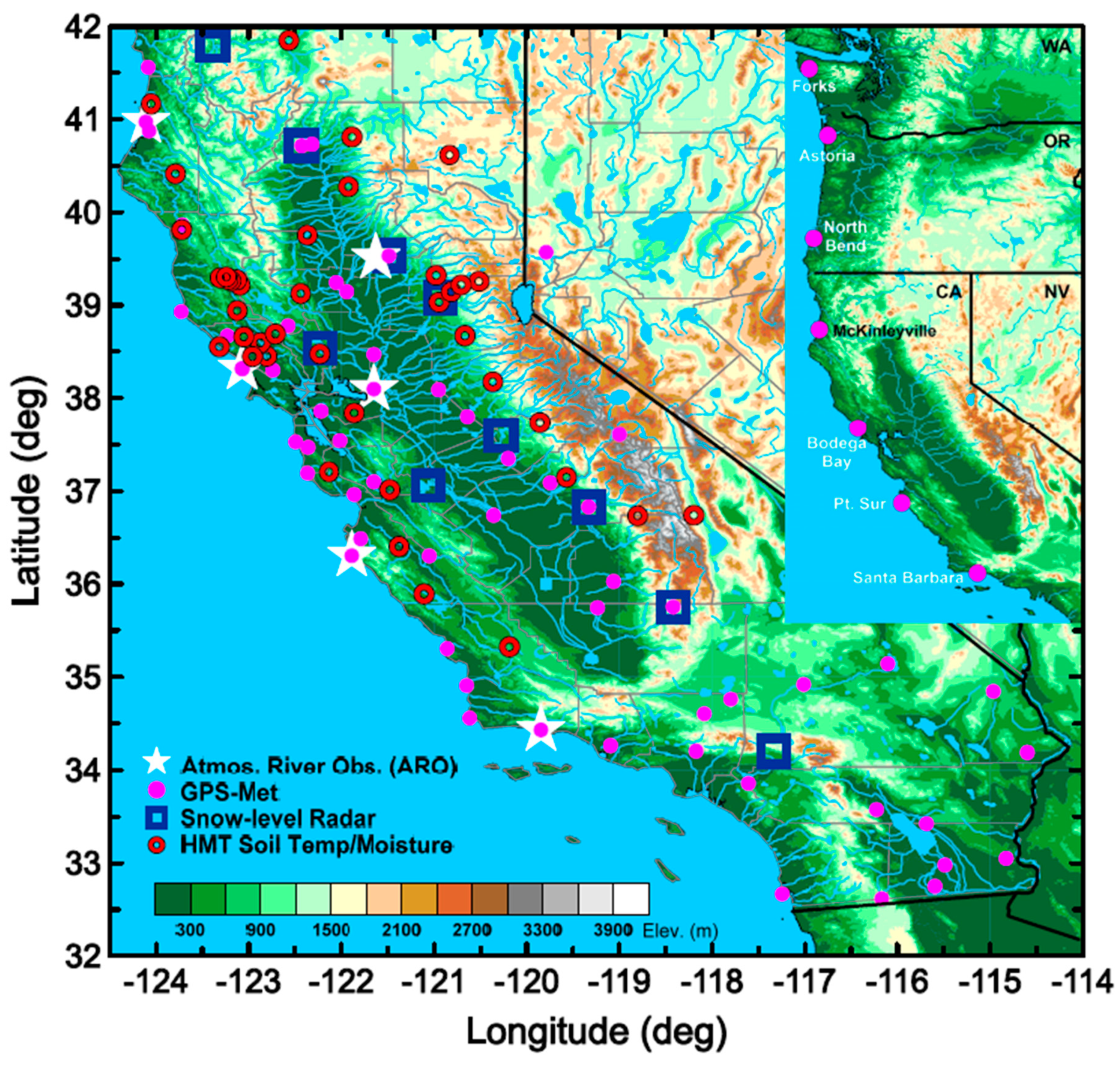
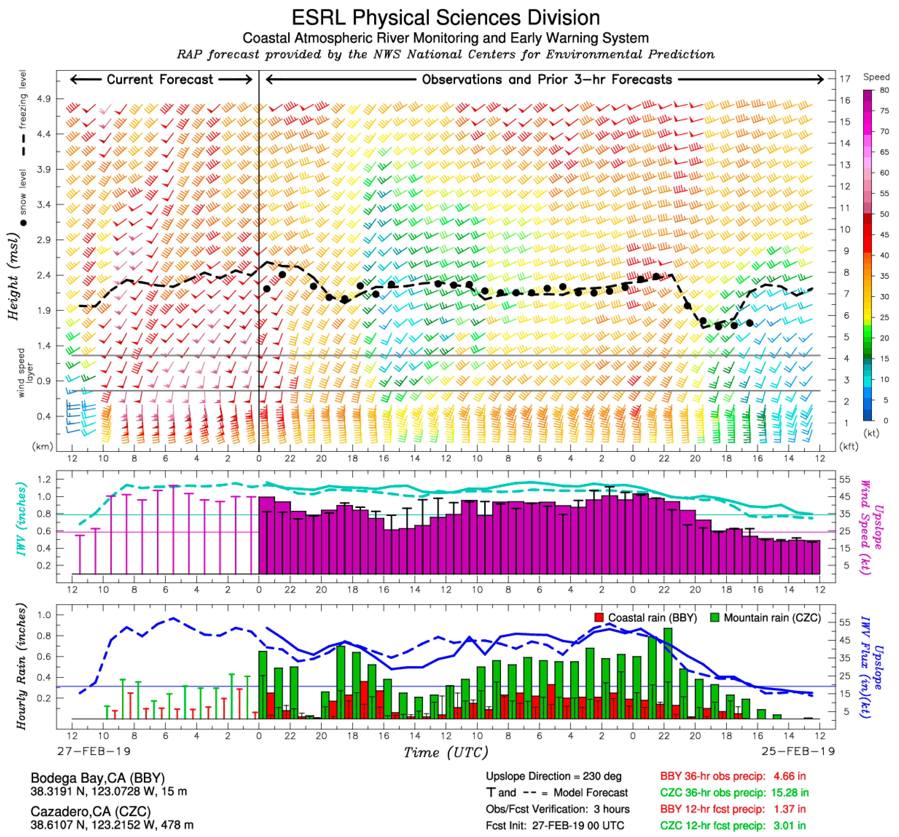
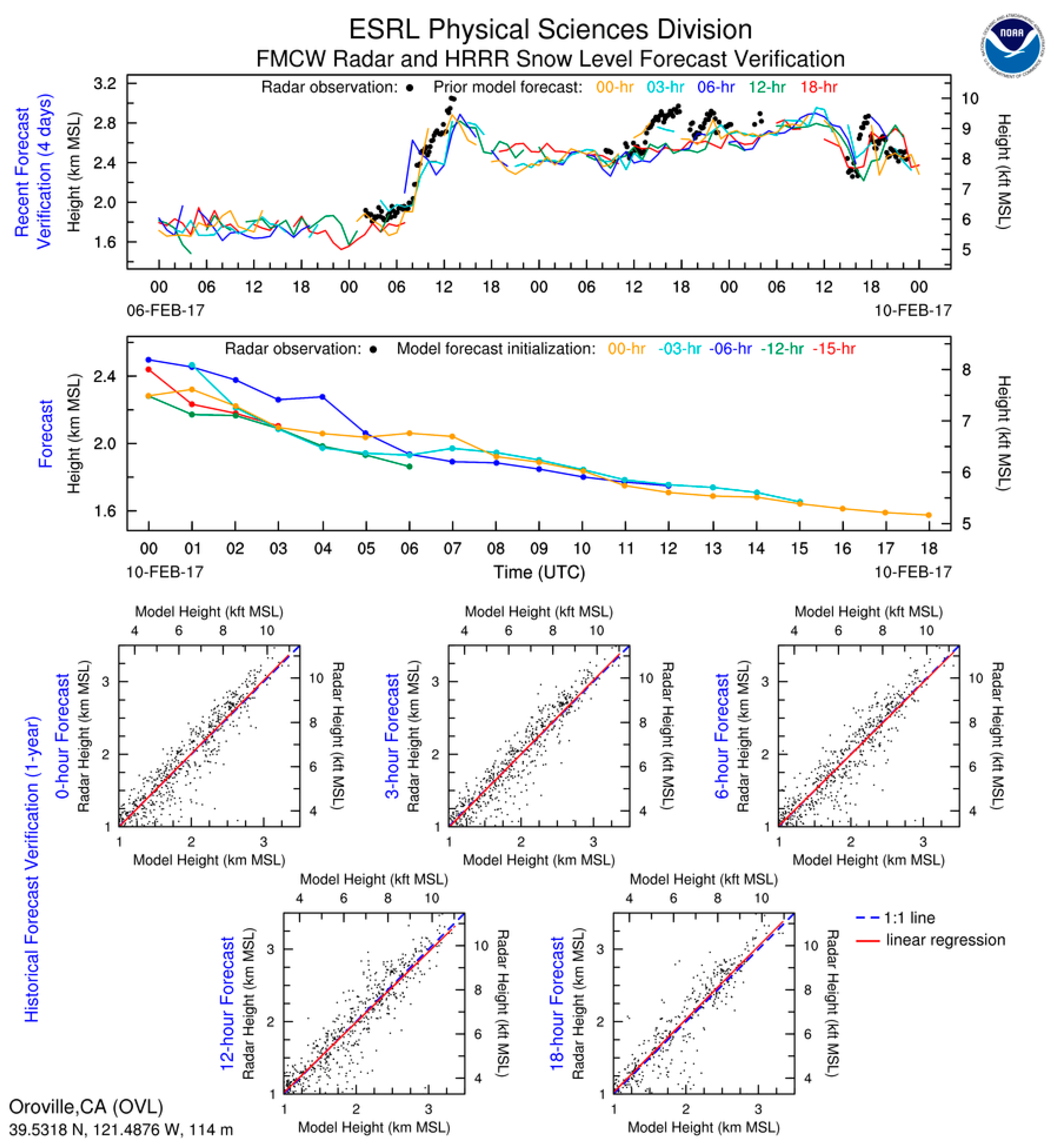
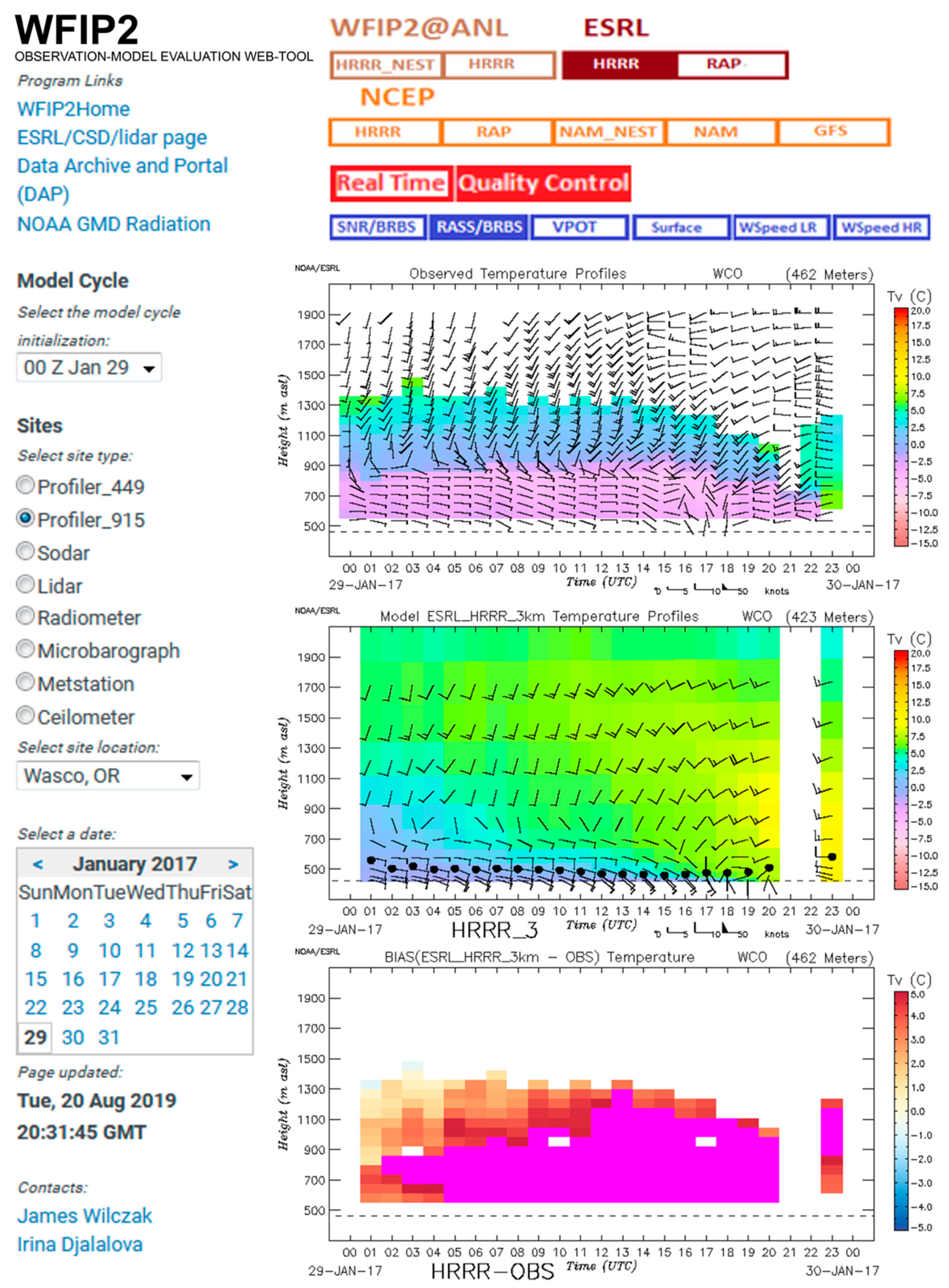
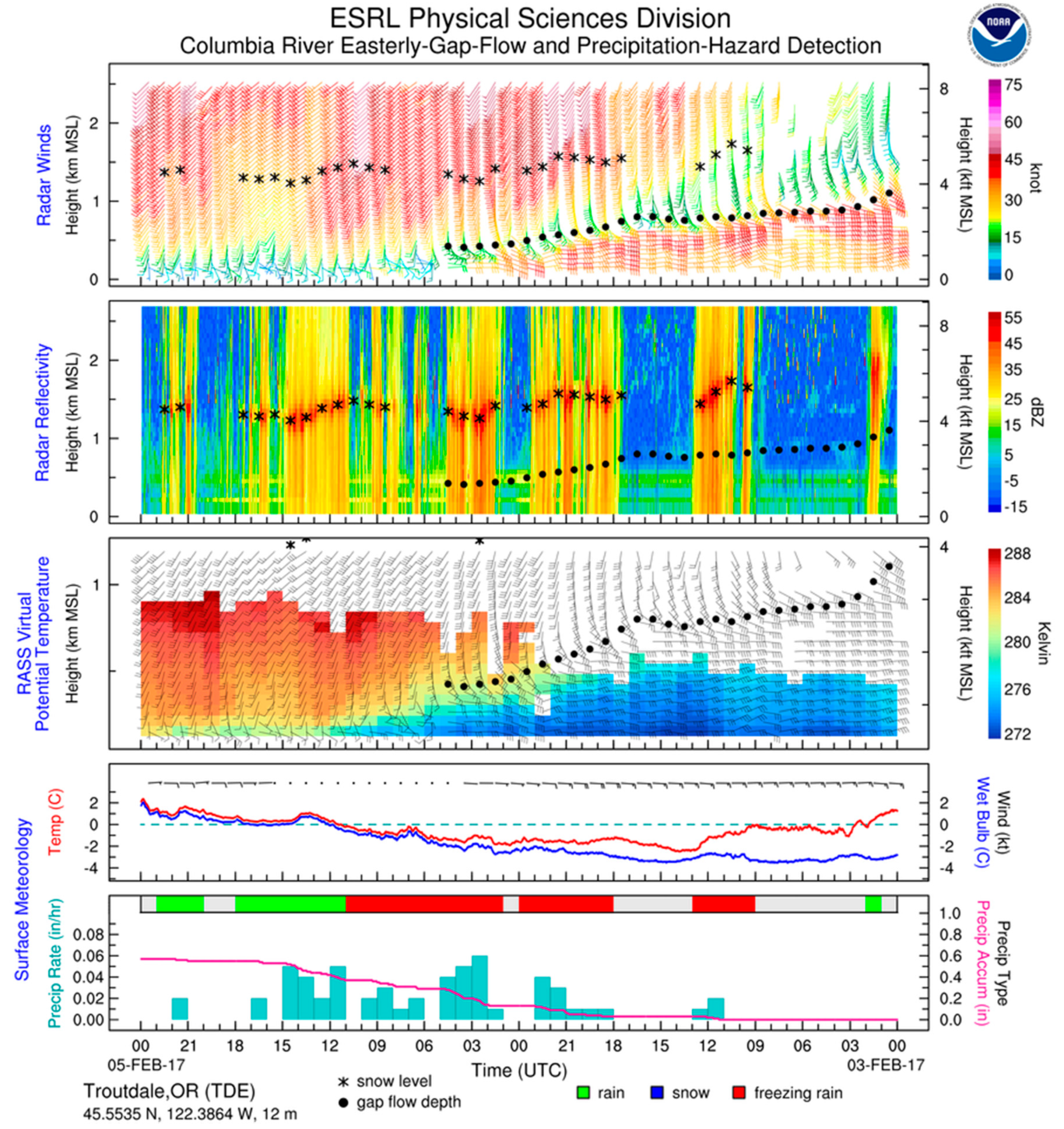
Table 1.
Instruments and parameters measured at HMT–West network sites. ARO stations include a 449-MHz or 915-MHz WP radar and all the instrumentation below. Other sites shown in Figure 1 have one or more of the instruments described below.
Table 1.
Instruments and parameters measured at HMT–West network sites. ARO stations include a 449-MHz or 915-MHz WP radar and all the instrumentation below. Other sites shown in Figure 1 have one or more of the instruments described below.
Wind profiler observations at fine temporal and vertical scale in the boundary layer
|
Radar reflectivity and Doppler vertical velocity (S-PROF and snow-level radars)
|
Surface met tower, GPS, surface measurements (2 min. avg.)
|
Soil Moisture
|
Derived products:
|
Table 2.
Select WP radar stations. Stations shown are examples from over 200 ephemeral WP deployments, chosen because of their long records or deployment in areas with few observations. WPs are typically co-located with a suite of other instruments (right column). Abbreviations: 449 (449-MHz WP radar); 915 (915-MHz WP radar) GPS-met (GPS meteorological station), soil moisture (SM); Smet (surface meteorological station); disdrometer (Disd); snow-level radar (SLR); S-PROF precipitation profiling radar (S-PROF); water vapor flux (WVF); rawindsonde (RAOB); microwave radiometer (MWR); * indicates an ongoing station. This information provided by the NOAA/OAR/ESRL PSD profiler library, which also provides information on other stations: https://www.esrl.noaa.gov/psd/data/obs/datadisplay.
| Project and Locations | Latitude, -Longitude (deg.), Elev (m) | Deployed (Month/Year) | Collocated Instruments |
|---|---|---|---|
| ARO/WFIP2 | |||
| Forks, WA | 47.98, −124.40, 95 | 6/2015 * | 449, GPS-met, SMet, SLR, SM, RASS |
| Astoria, OR 1 | 46.16, −123.88, 3 | 9/2015 * | 449, GPS-met, SLR, SM |
| South Bend, OR | 43.42, −124.24, 5 | 10/2015 * | 449, GPS-met, SLR, SM |
| Troutdale, OR | 45.55, −122.39, 12 | 9/2015 * | 915, GPS-met, RASS, Disd, SMet |
| ARO/HMT (CA) | |||
| McKinleyville | 40.97, −124.11, 56 | 11/2015 * | 449, GPS-met, SLR, SM |
| Bodega Bay | 38.32, −123.07, 15 | 3/2013 * | 449, GPS-met, SLR, SM |
| Pt. Sur | 36.30, −121.89, 10 | 10/2016 * | 449, 915, S-PROF, GPS-met, SLR, SM, |
| Santa Barbara | 34.43, −119.85, 2 | 8/2016 * | 449, GPS-met, SLR, SM |
| Oroville | 39.51, −121.63, 56 | 10/2017 * | 915, GPS-met, SLR, SM |
| Twitchell Island | 38.06, −121.65, 12 | 10/2017 * | 915, GPS-met SLR, SM |
| HMT- SE 2 | |||
| New Bern, NC | 35.08, −81.05, 3 | 6/2013–11/2015 | 449, S-PROF, GPS-met, Disd |
| Moss Point, MS | 30.47, −88.53, 6 | 6/2014–11/2015 | 915, GPS-met, WVF, |
| Old Fort, NC | 35.64, −82.16, 427 | 6/2013–10/2014 | 449, RASS, S-PROF, GPS-met, Parsival |
| Johns Is, SC | 32.70, −80.00, 15 | 6/2014–11/2015 | 915, GPS-met |
| Sydney, FL | 27.97, −82.23, 27 | 6/2014–11/2015 | 449, GPS-met |
| WFIP 3 | |||
| Valley City, ND | 47.03, −98.08, 378 | 6/2011–9/2012 | 449, Smet, GPS-met, WVF |
| Leeds, ND | 48.28, −99.40, 466 | 6/2011–9/2012 | 915, SODAR, Smet, WVF |
| Buffalo, SD | 44.43, −97.56, 877 | 6/2011–9/2012 | 449, SODAR, Smet |
| Ainsworth, SD | 42.58, −100.0, 793 | 6/2011–8/2012 | 915, SODAR, GPS-met, Smet, WVF |
| St James, MN | 43.98, −94.55, 324 | 6/2011–9/2012 | 915, SODAR, Smet |
| Brady, TX | 31.18, −99.33, 548 | 8/2011–9/2012 | 915, SODAR |
| Colorado City, TX | 32.47, −100.9, 665 | 7/2011–9/2012 | 915, SODAR |
| Lubbock, TX | 33.50, −102.0, 1018 | 3–12/2012 | 915, SODAR |
| Northeast & Texas Air Quality 4 | |||
| Pittsburg, PA | 40.48, −80.26, 335 | 6/2004–5/2005 | 915, SMet |
| Lunenberg, NS | 44.4, −64.3, 30 | 6/2003–5/2005 | 915, SMet |
| Plymouth, MA | 41.91, −70.73, 46 | 6/2002–5/2005 | 915, Smet |
| Beeville, TX | 28.37, −97.8, 75 | 6/2005–10.2006 | 915, Smet |
| El Paso, TX | 31.77, −106.5, 1160 | 6/2005–10/2006 | 915, SMet |
| Pacific 5 | |||
| Nauru | −0.54, 166.92, 11 | 11/1992–2/2003 | 915, SMet |
| Manus | −2.06, 147.42, 3 | 4/1992–2/2003 | 915, SMet |
| Kiritimati | 2.00, −157.40, 4 | 3/1990–8/2002 | 915 and 50-MHz WPs, SMet |
| Tarawa | 1.36, 172.92, 2 | 8/1994–2/2003 | 915, SMet |
| Arctic | |||
| R/V Oden, ACSE 2014 6 | 70–85, 19 to −156, 14 | 7–10/2014 | 449, RAOB, W-band, MWR, scanning lidar, flux tower, wave-height recorder, CTDs |
| R/V Oden, ASCOS 2008 7 | 77–90, 15 to −15, 14 | 8–9/2008 | 449, RAOB, scanning 5-mm radiometer, MMCR, MWR, flux tower, tethersondes |
| R/V Oden, AOE-2001 8 | 77–90, 10 to −150, 8 | 7–8/2001 | 915, S-PROF, RAOB, scanning 5-mm radiometer, ceilometer, on ice instruments 9 |
| Barrow, AK | 71.3, −156.6, 10 | 2–3/1997 | 449, RASS, RAOB |
| LEADEX 1992 10 | 73, −144, 0 | 3–4/1992 | 915, RAOB, RASS, surface met & energy budget, flux tower, ceilometer, SODAR |
1 Astoria was also occupied in 1993–96 and 2003–06 with a 915-Mhz radar. 2 Data for this experiment is archived at http://www.esrl.noaa.gov/psd/data/obs/datadisplay/, click on menu and select inactive sites. 3 The WFIP project included 12 WP radars and sodars (north and south), several lidars, & 71 surface met stations, see https://www.esrl.noaa.gov/psd/renewable_energy/wfip/. 4 Information on and additional instruments deployed in the New England Air Quality Studies: https://www.esrl.noaa.gov/csd/projects/neaqs and https://www.esrl.noaa.gov/csd/projects/2004; this study included measurements from the NOAA WP-3D aircraft and surface measurements using the R/V Ronald H. Brown. For the Texas Air Quality Study see [36]. 5 Selection of sites from the Trans-Pacific Profiler Network (https://www.esrl.noaa.gov/psd/psd3/boundary/MstToga/data_access.html), Nauru and Manus co-located with DOE- ARM sites; Tarawa also an WMO radiosonde site. 6 Arctic Clouds in Summer Experiment (ACSE), see [18]. 7 Arctic Summer Cloud Ocean Study (ASCOS); see [21]; included icebreaker cruise and drift. 8 Arctic Ocean Expedition 2001, see [20]. 9 On-ice instrumentation 2–21 Aug 2001: flux tower, tethersondes, microbarograph, ISFF station. 10 Arctic Leads Experiment (LEADEX, The LeadEx Group 1993.
© 2019 by the authors. Licensee MDPI, Basel, Switzerland. This article is an open access article distributed under the terms and conditions of the Creative Commons Attribution (CC BY) license (http://creativecommons.org/licenses/by/4.0/).
Share and Cite
MDPI and ACS Style
Ray, A.J.; White, A.B. The Hydrometeorology Testbed–West Legacy Observing Network: Supporting Research to Applications for Atmospheric Rivers and Beyond. Atmosphere 2019, 10, 533. https://doi.org/10.3390/atmos10090533
AMA Style
Ray AJ, White AB. The Hydrometeorology Testbed–West Legacy Observing Network: Supporting Research to Applications for Atmospheric Rivers and Beyond. Atmosphere. 2019; 10(9):533. https://doi.org/10.3390/atmos10090533
Chicago/Turabian StyleRay, Andrea J., and Allen B. White. 2019. "The Hydrometeorology Testbed–West Legacy Observing Network: Supporting Research to Applications for Atmospheric Rivers and Beyond" Atmosphere 10, no. 9: 533. https://doi.org/10.3390/atmos10090533
Note that from the first issue of 2016, this journal uses article numbers instead of page numbers. See further details here.