Abstract
Due to their rarity and intensity, Mediterranean Tropical-Like Cyclones (TLCs; also known as medicanes) have been a subject of study over the last decades and lately the interest has undoubtedly grown. The current study investigates a well-documented TLC event crossed south Sicily on November 7–8, 2014 and the added value of higher spatial horizontal resolution through a physics parameterization sensitivity analysis. For this purpose, Weather Research and Forecasting model (version 3.9) is used to dynamically downscale ECMWF Re-Analysis (version 5) (ERA5) reanalysis 31 km spatial resolution to 16 km and 4 km, as parent and inner domain, respectively. In order to increase the variability and disparity of the results, spectral nudging was implemented on both domains and the outputs were compared against satellite observations and ground-based stations. Although, the study produces mixed results, there is a clear indication that the increase of resolution benefits specific aspects of the cyclone, while it deteriorates others, based on both ground and upper air analyses. The sensitivity of the parent domain displays an overall weak variability while the simulations demonstrate a positive time-lag predicting a less symmetric cyclone with weak warm core. On the contrary, inner domain analysis shows stronger variability between the model simulations reproducing more distinct clear tropical characteristics with less delayed TLC development for most of the experiments.
1. Introduction
The Mediterranean basin is an area particularly prone to the generation of low-pressure systems [1]. The dominant type is extra-tropical cyclones, fueled by the baroclinic instability due to horizontal temperature gradients. However, cyclones with tropical features similar to those of tropical cyclones developed in the tropical Pacific, Atlantic and Indian ocean are observed occasionally. Given their similarity to tropical storms, they are referred to as “medicanes” (from the composition of the words MEDiterranean and hurrICANES). They are also often referred to as Tropical-Like Cyclones (TLCs) due to their distinct differences to tropical storms.
Medicanes are relatively rare phenomena, occurring about 1.6 times per year [2]. Given their rarity and the fact that they spend most of their lifetime over the sea, their tropical characteristics were not discovered until the 1980s [2]. However, their impacts can be severe as documented by [3], including floods caused by heavy rainfall and storm surge, crop disasters, drops of trees from strong winds as well as disasters in infrastructure, natural environment and human lives. Coastal and maritime areas are mostly vulnerable to these impacts rendering them potentially threatening for the tourism and shipping industries, which comprise a significant part of economic activity of the region.
Medicanes are warm-core low-pressure systems, driven by hydrostatic instability and evaporation from the sea surface over which they are formed. They are characterized by axial symmetry and the absence of fronts. Strong winds approach the center circularly and rise around it creating a spiral wall of clouds that surrounds the "eye", a small area with no clouds and no wind, like in tropical storms [4,5].
They have been found to develop above waters as cold as 15 °C, unlike tropical cyclones whose limit is considered to be 26 °C [6]. However, recent work Noyelle et al. 2019 [7], has shown that the sea surface temperature (SST) state has a strong influence on the intensity of TLCs, increases the probability of development and the lifetime. One more important difference to the tropical cyclones is that most medicanes, if not all, are initially formed as baroclinic cyclones, which is the dominant type of cyclones in the region. In an advanced stage of their life [5,8] they are converted into acquiring tropical characteristics due to favorable environmental conditions [9,10,11,12]. In this sense they can be classified near the subtropical cyclones [13]. In recent years the process of tropicalization has been the focus of several authors. A cut-off low in the mid-upper levels of the atmosphere has been detected near several medicanes [4,14]. This produces a pool of cold air with high potential vorticity which can enhance instability and deepen the surface pressure depression. This in turn intensifies circulation around the low pressure center thus enhancing the surface latent and sensible fluxes into being able to maintain the convection [9,10,15,16]. Chaboureau et al. 2012 [11], studying “probably the deepest medicane on record” pointed out the importance of the upper-level jet in the intensification of the system. However, in most medicane cases an upper-level jet is not present [5].
The geometric and physical characteristics of the Mediterranean basin limit the size and intensity that medicanes can reach. When they leave the sea, they lose their energy source, they gradually diminish and soon they disappear. Therefore, most medicanes travel less than 3000 km in less than 3 days. As a result, their radius and sustained winds usually do not exceed 200 km and 40 m/s respectively [14,17]. This wind speed would classify them in Category 1 of the Saffir-Simpson hurricane scale. Although significant progress has been made towards the understanding of medicanes, it is lagging behind in comparison to our understanding of tropical cyclones [18], particularly concerning the process of acquiring tropical characteristics [10,19]. This is not surprising given the much later beginning of their investigation and the much smaller number of historical phenomena that are available for studying.
Several authors have used limited area models to simulate historical medicanes aiming at a better understanding of the phenomenon or at investigating the capability of numerical weather prediction to capture its occurrence and development. This method is considered to have a potential to generate valuable results [20]. Being a mesoscale phenomenon, medicanes require high-resolution simulations in order to be accurately represented [5,11,17,21,22,23]. Increasing resolution improves the results, i.e., Akhtar et al. 2014 [20] performing nested LAM simulations found that at about 50 km resolution a medicane is not detected, at 25 km a pressure low with a warm core is detected but it is poorly represented, and at 9 km most medicane features can be reproduced and be well resolved. Also, there is a need for high-resolution SST fields spatially and temporally, either the ocean is coupled or prescribed [24].
The good quality of initial and boundary conditions is a key for accurate simulation of the occurrence and development of medicanes [24,25]. Davolio et al. 2009 [25] propose the use of a domain large enough and an initiation time early enough to capture the entire formation of the vortex. They found that even when the simulation runs on global forecast output, this configuration allows for better results than the usage of more recent output. This poses a challenge on real-time forecast of occurrence and development of medicanes because more computational resources and more time are required.
The development and the trajectory of medicanes depend mostly on the synoptic forcing, the internal structure and intensity depend mostly on the model configuration [25]. Coupled ocean-atmosphere models produce better than atmosphere-only models with prescribed SST when the atmospheric resolution is high [20]. Ricchi et al. 2017 [24] stressed the strong impact on the results by the choice of planetary boundary layer (PBL) scheme and of the dependence of the waves on surface roughness, especially when the medicanes approach the coast, which should be treated by sensitivity tests.
Miglietta et al. 2015 [26] performed a sensitivity analysis for a medicane event in Calabria, Italy in 2006 showing the variability of different subsets of physical parameterization schemes. That study illustrates that microphysical parameterizations exhibit the largest variability among the physics subsets, in agreement with several studies on tropical cyclone simulations [27,28,29]. Also, it is reported that the spatial resolution chosen for that study, 7.5 km, is sufficient to resolve explicitly the convection effects of cyclone evolution. In agreement with that [30], working with the same resolution explored an extensive sensitivity of physical parameterizations for the currently presented medicane event (TLC Qendresa). They illustrate that most of the tested simulations successfully represented the tropical nature of the medicane. Contrary to Miglietta et al. 2015 [26] they found that the intensity of the medicane is more sensitive to planetary boundary layer PBL parameterization. Although this spatial resolution has been proven adequate for resolving medicane events it is useful to investigate a higher resolution. TLC Qendresa was selected taking into account the sufficient literature and also the fact that it was one of the most intensive and characteristic medicane events in recent years [3].
Section 2 presents the model and the different configurations that were tested, as well as the observational datasets that were used for the evaluation of the simulations. Also, the methodology applied for the determination of the trajectory and structure of the medicane is described and finally a description of the event along with the synoptic environment is provided. In Section 3 the results of the simulations are presented and discussed. The conclusions of the study are reiterated in Section 4.
2. Data and Methodology
2.1. Model Configuration and Data
Weather Research and Forecasting (WRF) [31], version 3.9, is used for the simulations. The domain configuration applied comprises of one parent (D01) and one nested (D02) domain with one-way feedback (Figure 1). The domains have a bidirectional grid interval of 16-km and 4-km for the parent (D01) and inner domain (D02) respectively. Specifically, parent domain includes a large part of continental Europe while the nested domain is focusing on the Mediterranean region, with 284 × 231 and 849 × 569 grid points respectively. The 50 vertical levels are arranged according to terrain-following hydrostatic pressure vertical coordinates and they are denser in the lower troposphere. The model time-step is adaptive and it is determined between 30 s sand 162 s for the parent domain and between 15 s and 54 s for the inner domain, based on the horizontal resolution.
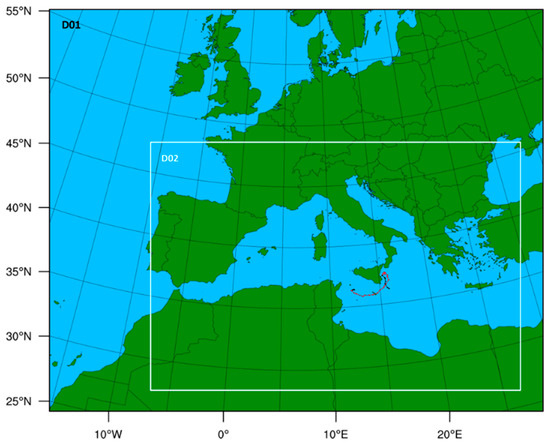
Figure 1.
Domains of case study.
A series of sensitivity tests are performed in order to assess the dependence of model performance on the choice of physics parameterization schemes. The control run (hereafter named “MAIN”) is using the Mellor-Yamada Nakanishi and Niino Level 2.5 (MYNN2.5) [32], the 5-layer thermal diffusion (5-L Thermal DIF) [33], Thompson 6-class with ice processes [34], Kain–Fritsch (KF) [35] and New Goddard [36] for the PBL, Land surface model (LSM), microphysics (MP), cumulus convection (CU) and radiation (LW and SW RAD) respectively. All other configurations differ from MAIN run in only one parameterization scheme (and their dependencies in some cases). In total, sixteen alternative configurations are tested, differing from MAIN in 5 subsets of physical parameterizations as shown in Table 1.

Table 1.
Weather Research and Forecasting (WRF) simulations’ configurations associated with physics parameterization schemes.
Concerning the PBL schemes, Yonsei University (YSU) [37], Mellor–Yamada–Janjic (MYJ) [38], Asymmetric Convective Model version 2 (ACM2) [39] and the Bougeault-Lacarrere (BouLac) schemes are involved, associated with the corresponding surface layers schemes, which provide the surface fluxes of momentum, moisture and heat to PBL scheme. For compatibility reasons with PBL schemes, surface layer (Sfclay) parameterizations have been adapted accordingly using the Mellor-Yamada Nakanishi and Niino scheme (MYNN) [40], the revised version of MM5 [41] and the ETA surface layer [42]. Regarding the cloud MP schemes, the options include Kessler simple warm-rain MP with no ice class [43], WRF single-moment three-class (WSM-3) and five-class (WSM-5) containing ice processes, [44,45,46], the Goddard 6-class scheme and the Purdue Li 5-class scheme [47] containing ice snow and graupel processes. For the land surface model, different setups involve Noah Land Surface Model [48,49] and RUC Land Surface Model and Noah-MP (multi-physics) [35]. The sub-grid-scale effects of convective clouds the options are set mainly to Betts–Miller–Janjic Scheme (BMJ) [50], Grell 3D (G3D) and Grell ensemble convection scheme [51]. Finally, for the long-wave and short-wave radiation schemes, five different options are used in this case study; RRTM scheme [52] and its newer version of RRTMG schemes [53], Dudhia [54], only for short-wave scheme, GFDL [55] and Community Atmosphere Model (CAM) scheme [56]. The parameterization schemes used in each one of the sensitivity test simulations is presented in Table 2.
Table 2.
WRF model configuration options for: control run, microphysical (MP), longwave Radiation (LW_RAD), shortwave Radiation (SW_RAD), land surface model (LSM), surface layer (Sfsclay), planetary boundary layer (PBL) and cumulus (CUM) experiments. Only the options different than the control run are shown.
The 17 sensitivity test simulations are initialized at 00:00 UTC on November 6, 2014, with 12 h of model spin up time until 00:00 UTC on November 10, 2014. The initial and boundary conditions are provided by ERA5 re-analysis data, derived from the European Center for medium range Forecast (ECMWF). ERA5 dataset has a spatial horizontal resolution of 0.28° × 0.28° (approximately 31 km spacing grid) and temporal incorporation in the model performed every 3 h with 37 isobaric atmospheric levels and 4 below land surface.
In addition to that, remote sensing data are used in order to validate the sensitivity simulations with regards to cyclone tracks and phase diagrams (hart). More specifically, Rapid Scan High Rate SEVIRI Level 1.5 Image Data derived from the Spinning Enhanced Visible and InfraRed Imager (SEVIRI) of European Organization for the Exploitation of Meteorological Satellites (EUMETSAT) is used to derive the cyclone center positions from the infrared 10.8 μm and from the visible 0.6 μm bands through the MSGView software [57]. The trajectory derived by the satellite imagery, complemented by the trajectory as derived by the ERA5 dataset for the other timesteps, is referred to as Combined Track (C-Track) throughout the paper. C-Track is presented as a black line in Figure 1.
2.2. Spectral Nudging
A simple form of data assimilation has been introduced in WRF including three modes of nudging; analysis (AN), spectral (SN) and observational (ON) nudging [58]. The current research focuses on investigating the optimal configuration with regards to physical parameterization schemes and spatial horizontal resolution and therefore, it is important to maintain the variability of physical parameterizations while improving the accuracy of the simulations. Spectral nudging has proven to be dampening physical parameterizations variability less than analysis nudging [59]. Also, studies for regional climate modelling have shown that analysis nudging is less efficient for sensitivity analyses in high resolution as it results in extinguishing fine-scale variability [60]. Additionally, spectral nudging can fade out extreme events as it drives the model toward a smoother, larger-scale state [61]. In agreement with the literature the key point is to nudge the coarse-scale components of the atmospheric fields toward the initial and boundary conditions, whilst the fine-scale components remain open to be implicitly or explicitly resolved by the model. After testing different nudging configurations in the control run the present study uses SN for nudging the simulations of both D01 and D02 domains with the input data. The model assimilates u and v velocity components along with air temperature only for vertical sigma levels above the 850 hPa layer in order to, first, maintain the large-scale circulation close to reanalysis data and leave the wind components undisturbed to interact with topography in the PBL [26]. Finally, in SN the wave number is set for zonal and meridional directions to define the wavelength above which the model will be nudged using the input reanalysis data, leaving the smaller scales undisturbed. For the current study the wave numbers are selected to correspond to spatial scales of 908 × 924 km2and 1132 × 1138 km2 for the parent and inner domain respectively.
2.3. Phase Space Diagrams
The main tool used for the characterization of low pressure systems is the phase space diagrams of Hart [13]. The evolution of a system’s structure is depicted in a 3-D phase space defined by the lower layer thermal wind (900–600 hPa, VTL), the upper layer thermal wind (600–300 hPa, VTU) and asymmetry parameter (B). The calculation of asymmetry parameter is performed in a circle around the center of low-pressure. The circle is divided in the right and left semicircles according to the motion of the center, i.e., to the trajectory of the storm. Asymmetry parameter, B, is the difference of the mean 900–600 hPa layer thickness in the right and left semicircles. As a number of researchers have proposed [9,10,22] the calculations were performed in a circle of 200 km radius. This radius is more appropriate for the Mediterranean region than the 500 km proposed by Hart who was focused on the storms of the tropical oceans which have a larger horizontal extent. The Hart phase space is usually projected by using two diagrams. Here, to avoid repetition, only one diagram is used with the two thermal wind parameters in the axes and the asymmetry is provided by the shade of the points.
In order to reduce noise in the calculation of the three phase space parameters, the grid points that lie near the edge of the calculation area were assigned a weight that was reduced linearly from half grid interval within the area to half grid interval outside the area. Also, the designation of the left and right semicircle for the calculation of asymmetry parameter, B, was not based on the trajectory direction which is quite noisy. Instead the calculation was performed for all directions at an interval of 1 degree and B was chosen as the highest positive difference of the left and right semicircle. This solution is in line with the rationale of Hart [13] but the values of B that it produces are always positive and slightly higher than the values usually produced by other researchers. Therefore, in our analysis we consider that axial symmetry is indicated by B values of 15 m or lower, instead of 10 m as proposed by Hart [13].
In order to improve the phase space diagrams, a prior step was added, using the sea-level pressure (SLP) gridded field to calculate the exact position of the low-pressure center with sub-grid accuracy. More specifically the grid point with the lowest pressure is located and subsequently, an inverted cone is fit to the SLP field by applying an iterative method with varying axis coordinates, apex height and aperture, which correspond to the low-pressure center coordinates, minimum pressure and horizontal pressure gradient away from the center respectively. A weight is applied in each iteration to maximize the influence of the grid points closest to the cone axis and to reduce exponentially the influence of grid points far from it. Essentially, this method makes use of the assumption of axial symmetry of the SLP field near a low-pressure center with tropical characteristics to expand the calculation into including several grid points, thus achieving higher precision. The resulting trajectories are smoother than the initial ones in every case thus evidencing the added value of the method. The method produces results for extra-tropical systems as well but they are considered less credible since the assumption of axial symmetry is no longer plausible and convergence is slower. All trajectories of this paper were calculated using this method, except for the part of the C-Track that was based on satellite observations. The creation of the phase space diagrams was based entirely on these trajectories.
2.4. Case Study (Synoptic Overview)
The low-pressure system under study developed in the Ionian Sea on 7–8 November 2014 causing significant damages in the Italian islands of Lampedusa and Sicily due mostly to strong winds and to rainfall (Figure 2). The Free University of Berlin assigned to it the name Qendresa. A brief description is provided here. Carrió et al. 2017 [9] and Pytharoulis et al. 2018 [30] provide further details and a thorough analysis can be found in Pytharoulis 2018 [22].
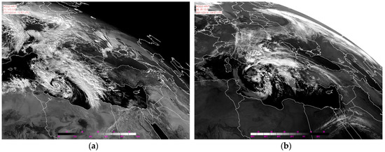
Figure 2.
EUMETSAT Meteosat Second Generation-3 satellite images of (a) the visible channel (0.6 μm) on November 7th 2014, 12:57 UTC and (b) the infrared channel (10.8 μm) on November 8th 2014, 04:57 UTC.
On the previous day, November 6th, an elongated trough extended in mid-troposphere from western Europe to western Sahara with a cold front developed along its eastern flank (Figure 3a). A closed circulation was formed near the tip of the trough and it propagated east towards the western gulf of Sirte and then north towards Sicily. This provided a pool of strong potential vorticity as well as cold air aloft (Figure 3b,c) that is known to favor the development of medicanes [10,15,16]. This was the synoptic environment that affected the parent low of Qendresa when it emerged between western Libya and the western gulf of Sirte.
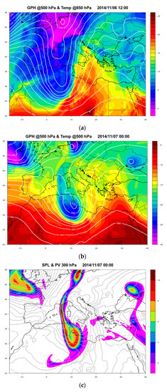
Figure 3.
(a) Geopotential height at 500 hPa (contour, gpm) and temperature at 850 hPa (shaded, °C) at 12:00 UTC, November 6th, 2014; (b) geopotential height (contour, gpm) and temperature (shaded, °C) at 500 hPa at 00:00 UTC, November 7th, 2014, and (c) sea-level pressure (contour, hPa) and potential vorticity at 300 hPa (shaded, PVU) at 00:00 UTC, November 7, 2014. Data are based on ERA5 reanalysis
The surface depression underwent a rapid deepening during the night between the 6th and the 7th of November (Figure 4, black dashed line). In the ERA5 dataset this depression amounts to 10.9 hPa in 6 h, from 1002.7 at 21:00 UTC to 991.8 at 03:00 UTC. The minimum pressure continues to drop until 05:00 UTC, reaching 991.3 hPa. Pytharoulis 2018 [22] using ECMWF analysis, which has higher spatial resolution, 0.125°, but lower temporal resolution, 6 h, found a similarly abrupt drop of the minimum pressure. However, he found that the minimum pressure drops further to 985.5 hPa at 12:00 UTC of November 7th. This explosive deepening was triggered by the PV anomaly in upper troposphere. The initial deepening enhanced the air circulation and evaporation at the surface. Within hours, latent heat release from rising air become a significant driver as well and the tropical-like air circulation cell became sustainable [9].
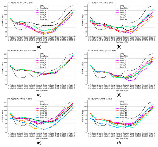
Figure 4.
Minimum mean sea-level pressure (MSLP) of PBL/LSM simulations: (a) D01 (parent domain) and (b) D02 (nested domain), MP simulations: (c) D01 and (d) D02 and CU/RAD simulations: (e) D01 and (f) D02. The ERA5 (black dashed line) and control run (setup-MAIN–black solid line) are also shown.
A cloud-free area corresponding to the “eye” is apparent in the satellite imagery before 12 UTC. In the following hours the medicane moved eastwards and between 16:00 and 17:00 UTC it crossed Malta allowing for the observation of some impressive time-series in Luca station, documented in Carrió et al 2017 and Pytharoulis 2018 [9,22]. After that, it veered towards the northeast and then north moving around Sicily until it reached the latitude of Catania (~37.5° N). At this point it turned southwest approaching the island. It briefly reached land between Syracuse and Augusta (~37.2) between 4:30 and 6:00 UTC without progressing beyond the coastline (Figure 2b). After landfall the tropical characteristics of the low-pressure system were lost and it left the island heading southeast.
The phase space diagram for medicane Qendresa is presented in Figure 5. The parent low pressure system is clearly extra-tropical in the beginning of November 7th. However, the thermal wind in the lower layer and subsequently in the upper layer underwent a strong positive change which coincides with the quick drop of pressure minimum. After a 2-h interval the thermal wind stabilized in the positive quadrant. At 12:00 UTC of November 7 asymmetry B also reached low values so all three Hart scores reached the region of systems with tropical characteristics. This continued until 05:00 UTC of the 8th, except for the lower layer thermal wind that reached near zero and slightly negative values near midnight. From 06:00 UTC only parameter B indicates tropical characteristics, probably due to residual axis-symmetrical structure.
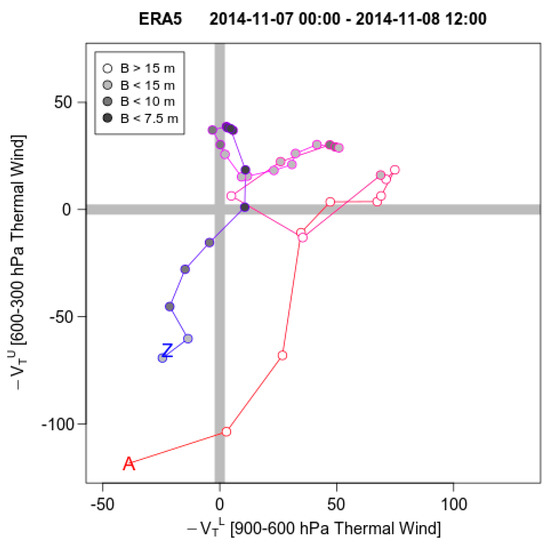
Figure 5.
Phase space diagram of lower layer thermal wind (900–600 hPa, −VTL) versus upper layer thermal wind (600–300 hPa, −VTU). The asymmetry parameter, B, is denoted by the shade in the interior of the circles according to the legend, so that white circles correspond to a non-symmetric core and darker grey circles correspond to a more symmetric core. The color of the lines and circles changes with time from red to blue. Data are based on the ERA5 hourly dataset from 00:00 UTC, November 7, 2014 to 12:00 UTC, November 8, 2014.
3. Results and Discussion
The sensitivity of the WRF model experiments is presented in this section. The analysis is presented separately for (a) MP, (b) PBL/LSM and (c) CU/RAD parameterization schemes and the discussion focuses on the influence of spatial horizontal resolution on the development and evolution of the medicane.
3.1. Planetary Boundary Layer and Land Surface Model Simulations
Figure 6 presents the trajectories of Qendresa in the PBL/LSM group of experiments along with setup-MAIN and the C-Track from 06:00 UTC on November 7 to 12:00 UTC on November 8. The spread of the D01 trajectory paths is moderate and rather uniform throughout the cyclone’s route. In all experiments the low-pressure center emerges 1–1.5° to the north from the observed center, near the western tip of Sicily. The northern shift is gradually reduced as the low-pressure system moved eastwards until the tracks meet the observed track (setup-MAIN) or come less than 0.5° away shortly after its passage through Malta. Such discrepancies between model results and observations are to be expected in modeling studies. For example, Pytharoulis et al. 2018 [30], working on the same TLC, demonstrated a northern discrepancy at the initial locations which is gradually reduced throughout the cyclone lifetime. Also, Carrio et al. 2017 [9] simulated the same event with large discrepancies. It is also worth noting that simulations with limited area models (LAMs) commonly produce results that may improve later because of the continued influence of the boundary conditions. The northern shift of our simulated trajectories is reduced during the tropical phase of the cyclone which is the focus of this paper.

Figure 6.
Trajectories of the Tropical-Like Cyclones (TLC) from 7 November at 06:00 UTC to 8 November at 12:00 UTC (depicted hourly) as predicted from the model PBL/LSM experiments in the low (a) and high (b) resolution domain. The “combined” track (black line) and control run (setup-MAIN-blue line) are also shown. The position of the low-pressure center is denoted with solid dots every six hours, i.e., at 06:00, 12:00, 18:00 UTC November 7, and at 00:00, 06:00, 12:00 UTC November 8th, and with open dots in all other hours.
All experiments follow the observed track in its northward stretch in the east of Sicily, short stay there and southeast departure. However, the northern reach of all tracks is about 0.5° short comparing to the observations. Also, although the simulated tracks converge with the observed after the passage over Malta, setup-MAIN, setup-1 and setup-14 lag behind by about 2 h and at the end of the track they are ahead by 4 h, except for setup-MAIN that is ahead by only 2 h, probably as a result of their shorter northern reach along the eastern coastline of Sicily.
The behavior of the PBL/LSM group trajectories is similar in the D02 domain, except that their spread is much larger after they reach the eastern edge of Sicily and until noon of November 8th. The northern shift in the beginning of the trajectories is slightly smaller than in the D01 domain. Setup-MAIN trajectory splits to the south of the group, it approaches the C-Track first and it even reproduces the passage over Malta, although with 1hour delay. Setup-3 track splits to the north of the group and approaches Sicily and at 23:00 UTC of November 7 a short landfall occurs in the gulf of Avola, after which it moves southeast re-joining the group. The mean distance of the trajectories to the C-Track (Figure 7) is clearly reduced in the higher resolution simulations of setups 1, 2 and 14 (LSM) by 12 to 24%. On the contrary, for setup-3, which was the most prominent outlier in the D02 simulations, and for setup-4, also an outlier, the mean distance increased by about 26% and 4% respectively. Timeseries of the distance between simulated and observed trajectories (not shown) confirm that this increase is attributed to the part of the trajectory following the landfall for setup-3 and to the period leading to and immediately after the short northern reach to the east of Sicily for setup-4.
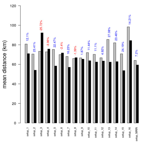
Figure 7.
Average track error (km) from 7 November at 06:00 UTC to 8 November at 12:00 UTC (hourly) between the “best” track of TLC, as derived from ERA5 and satellite imagery, and the model experiments for the low (grey bars) and high (black bars) resolution domain. The difference (%) between the two domains is depicted above the bars.
The phase space diagrams (Figure 8) of the PBL/LSM group of simulations also exhibit similarities among them. In agreement with the observations the system acquires tropical characteristics beginning with a positive thermal wind at the lower layer (900–600 hPa), VTL, which reaches its maximum value. In the next few hours the thermal wind of the upper layer (600–300 hPa), VTU, also acquires a positive value while asymmetry, B, is reduced under the symmetry threshold, taken here to be 15 m, signifying that the system acquires a deep warm-core.
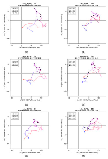
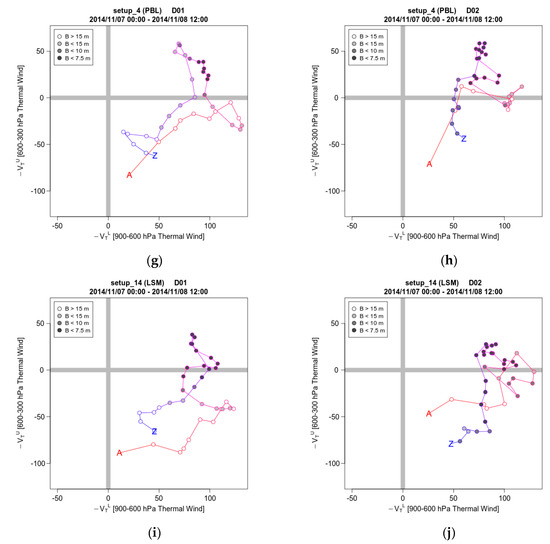
Figure 8.
Phase space diagrams of −VTL (900–600 hPa) against −VTU (600–300 hPa) as predicted from model PBL/LSM experiments in D01 for: (a) setup_1, (c) setup_2, (e) setup_3, (g) setup_4, (i) setup_14 and in D02 for: (b) setup_1, (d) setup_2, (f) setup_3, (h) setup_4, (j) setup_14. Symmetry B is denoted by the shade of circles.
Table 3 was created based on the values of the phase space parameters. According to Table 3, all D01 simulations of the PBL underestimate the duration of the tropical phase. The PBL simulations are close to the observed with a deep symmetric warm-core sustained for 13 to 14.5 h. In the LSM simulation (setup-14) the underestimation is stronger as the duration of the tropical phase is only 10.5 h. However, in simulation MAIN the tropical phase is very weak and lasts less than 4 h, which in some studies is not enough for the event to be characterised as a medicane [43]. As seen in Figure 9, this can be attributed to the thermal wind of the upper layer, VTU, signifying that a shallow core is formed but it does not deepen for long enough.
Table 3.
Time of first and last occurrence of a deep symmetric warm-core as well as duration in all simulation experiments and in the ERA5 dataset according to the phase space diagrams. Init: initial occurrence in UTC time on November 7th, Fin: last occurrence in UTC time on November 8th, Dur: duration in hours, Diff: difference in duration between the D01 and D02 simulations for each model setup. All numbers are given with half hour precision.

Figure 9.
Phase space diagrams of −VTL (900–600 hPa) against −VTU (600–300 hPa) as predicted from control (setup-MAIN) experiment in (a) D01 and (b) D02 domain. Symmetry B is denoted by the shade of circles.
A symmetric deep warm-core is also clearly reproduced in all D02 simulations. It emerges in all setups before 13:00 UTC of 7 November and its duration is in all cases longer than in the respective D01 simulations, thus achieving a better agreement with observations. In particular setup-MAIN produced a deep warm-core that lasted 13.5 h, a stark improvement in comparison to the 3.5 h in the D01 simulation. The improvement was also significant for setup-14, which uses MYNN2.5 and Unified Noah for PBL and LSM schemes respectively, in which duration increased from 10.5 to 14.5 h. The longest duration, 17.5 and 17 h, was achieved by setups 2 and 4 respectively. Setup-2 which used the YSU non-local closure PBL scheme seems to have the best overall performance between the experiments of not only the PBL/LSM subset but also the entire ensemble of the current study. It demonstrates a significant track error reduction in D02 (23.41%) as well as an elimination of the 1-hour time-lag of D01, resulting in the lowest tracking distance of 52.51 km. This partially follows the results of Pytharoulis et al. 2018 [30] that used YSU PBL scheme in the control run configuration resulting in a good overall performance compared to other model configurations.
3.2. Microphysics Sensitivity Simulations
The trajectories of the Microphysical experiments are presented in Figure 10. The spread among the trajectories of this group, including setup-MAIN, is much smaller than in the PBL/LSM group, especially in the D01 domain. As in the PBL/LSM experiments, the northward shift in the first part of the tracks is smaller in the D02 domain, so much so that all trajectories pass over Malta or very close. The only trajectory that stands out in D01 is setup-5 which deviates upon reaching off the eastern coast of Sicily and thereafter.
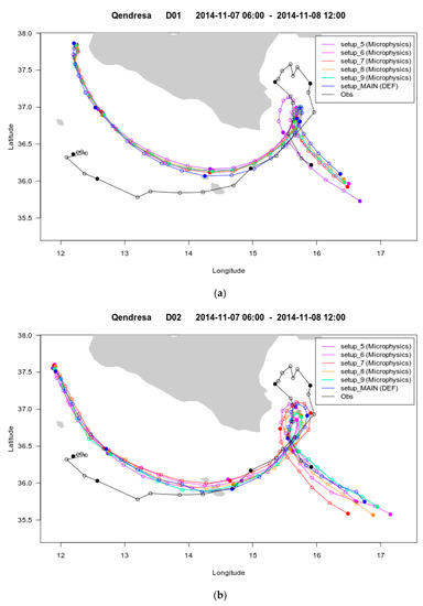
Figure 10.
Trajectories of the TLC from 7 November at 06:00 UTC to 8 November at 12:00 UTC (depicted hourly) as predicted from the model MP experiments in the low (a) and high (b) resolution domain. The “combined” track (black line) and control run (setup-MAIN - blue line) are also shown. The position of the low-pressure center is denoted with solid dots every six hours, i.e., at 06:00, 12:00, 18:00 UTC November 7, and at 00:00, 06:00, 12:00 UTC November 8, and with open dots in all other hours.
The spread is greater in the D02 experiments, especially from the northern stretch of the tracks off the east coast of Sicily, whose northernmost latitude varies, and thereafter. The smallest mean distance from the C-Track is found in the d02 simulations of setup-7 (55 km) and setup-5 (52 km), which are also the setups with the greatest percentage reduction of mean distance in comparison to the d01 trajectories. Setup-5, is able to minimize the distance error and also achieve a significant improvement in high resolution grid, both in cyclone intensity and track error. This is in line with Miglietta et al. 2015 [26] who found that, Kessler MP scheme was able to appropriately predict the intensity and track of an intense cyclone in southeastern Italy in 2006. The small differences of the MP simulations to the default simulation (MAIN) is evidence that the results are not very sensitive to the choice of MP scheme, especially in the lower resolution domain, with the exception of the Kessler scheme.
The phase space diagrams of the MP experiments (Figure 11) reveal that in the D01 domain a deep symmetric warm-core is formed in all experiments but it emerges late on the 7 of November and is short lived. As is the case in the PBL/LSM experiments, a shallow symmetric warm-core is formed early enough but the values of upper layer thermal wind, VTU, are too small. In the D02 simulations –VTU is more positive and the duration of the tropical phase is 12.5 to 14 h.
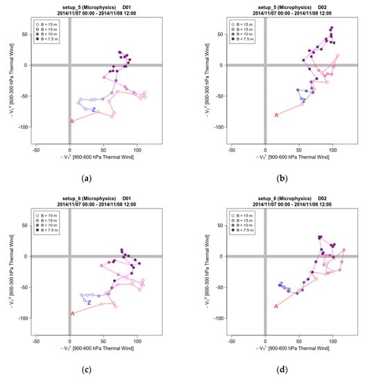
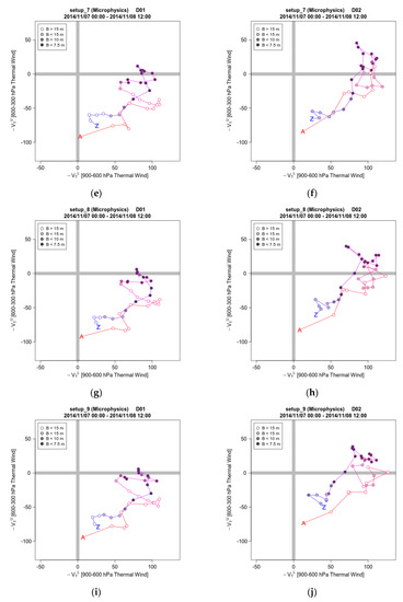
Figure 11.
Phase space diagrams of –VTL (900–600 hPa) against –VTU (600–300 hPa) as predicted from model MP experiments in D01 for: (a) setup_5, (c) setup_6, (e) setup_7, (g) setup_8, (i) setup_9 and in D02 for: (b) setup_5, (d) setup_6, (f) setup_7, (h) setup_8, (j) setup_9. Circles show the position at hourly intervals while filled circles denote the position when the symmetry is less than 10 m.3.3. Convection and Radiation sensitivity simulations.
The trajectories of the CU/RAD experiments are presented in Figure 12. Most trajectories are similar to those of the previous groups. Setup-16 is a prominent outlier. Its trajectory deviates from the group taking a more northern path leading to the southeastern tip of Sicily (capo Passero). After a short landfall at 22:00 UTC of November 7 it heads southeast and rejoins the group. The deviation of setup-13 is less pronounced and it rejoins the rest of the CU/RAD group before a landfall occurs. Consistently with the previous groups, the northern shift in the beginning of the trajectories is less pronounced in D02 domain. In the D02 domain setup-13 in not an outlier, while setup-16 remains an outlier following largely the track of the D01 simulation except without a landfall.
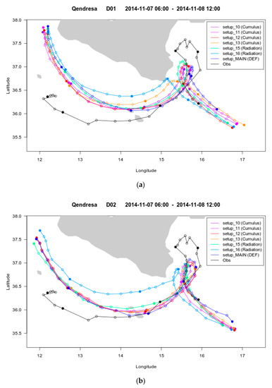
Figure 12.
Trajectories of the TLC from 7 November at 06:00 UTC to 8 November at 12:00 UTC (depicted hourly) as predicted from the model CU/RAD experiments in the low (a) and high (b) resolution domain. The “combined” track (black line) and control run (setup-MAIN - blue line) are also shown. The position of the low-pressure center is denoted with solid dots every six hours, i.e., at 06:00, 12:00, 18:00 UTC November 7, and at 00:00, 06:00, 12:00 UTC November 8th, and with open dots in all other hours.
The phase space diagrams for the CU/RAD group are presented in Figure 13. Setup-13 is again an outlier and is discussed in the following paragraph. The other CU simulations also produce a symmetric warm-core that is sustained for 11-12 h. In the case of setup-10 this core clearly represents a TLC. In setups 11 and 12 it is disputable whether the core becomes deep for long enough signifying the emergence of a TLC. In setup-12 the values of VTU are marginally positive for about 10 h while in setup-11 the value of VTU is at the same time slightly smaller and it fluctuates around zero. If the criteria of Hart [13] are to be considered accurate, then a TLC was formed in setup-12, although not particularly strong, and not in setup-11. However, we consider that in both cases it is debatable whether a TLC was formed or not. The times and duration in Table 3 refer to the case that a TLC was formed. In the D02 domain in all CU simulations, including setups 11 and 12, a deep symmetric warm-core is clearly formed and lasts for 12-14 h.
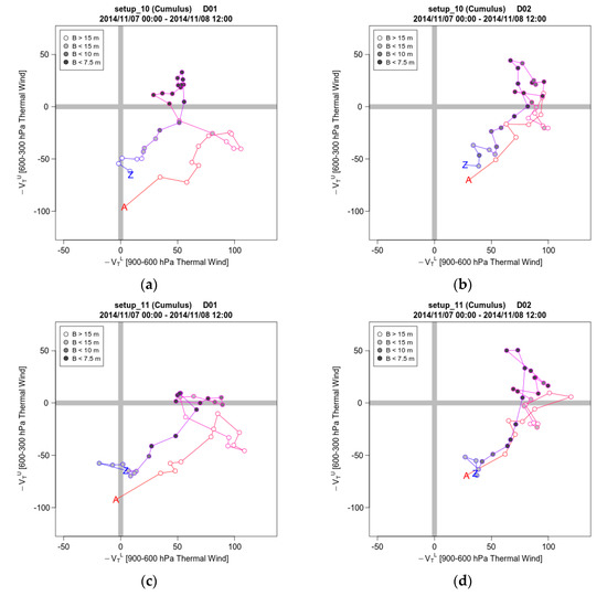
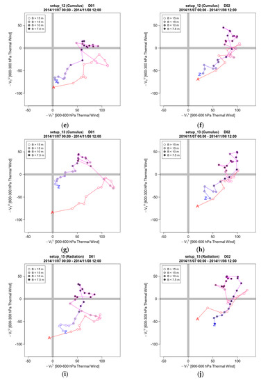
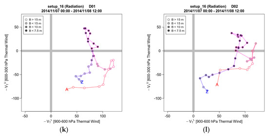
Figure 13.
Phase space diagrams of −VTL (900–600 hPa) against –VTU (600–300 hPa) as predicted from model CU/RAD experiments in D01 for: (a) setup_10, (c) setup_11, (e) setup_12, (g) setup_13, (i) setup_15, (k) setup_16 and in D02 for: (b) setup_10, (d) setup_11, (f) setup_12, (h) setup_13, (j) setup_15, (l) setup_16. Circles show the position at hourly intervals while filled circles denote the position when the symmetry is less than 10 m.
Setup-13 produces the longest sustained tropical phase of all the d01 experiments, 16 h. This lifetime is longer by at least 4 h than the other CU experiments and by 1.5 h longer than any experiment of this paper. It is also the only experiment in which the increase in resolution causes the tropical phase duration to decrease by 2 h while in all other experiments it increased by at least 1.5 h. The reason for this extraordinary behaviour is probably the outlier trajectory, including as short landfall, in the D01 experiment and not on the properties of the Grell 3D Ensemble scheme. It is well known that the effect of a landfall on a medicane is to cause its weakening and dissipation [11,17,20]. This simulation provides evidence that a short landfall may lead to the opposite result, i.e., to prolong its lifetime of a medicane, perhaps by reducing the rate at which it consumes its available energy. Further research could enlighten whether the short landfall was indeed the reason for the elongation of the TLC’s lifetime. The behavior of setup-13 simulation is partially in agreement with Pytharoulis et al. 2018 [30], who found that using Grell 3d CU scheme, the track error is maximized for the same TLC.
In the RAD simulations, tropical phase duration behaves similarly to the CU simulations in the D01 domain. The performance of setup-15 which uses the RRTM and Dundhia schemes for resolving LW and SW radiation respectively, lies in consistence with Moscatello et al. 2008 [62], who successfully simulated the cyclone in southeastern Italy in 2006, with a 16 km resolution grid. However, in the D02 domain, only setup-16 behaves like the respective CU simulations. Setup-15 produces a symmetric deep warm-core with 5.5 h longer life-time and particularly stronger, especially concerning the upper layer thermal wind VTU. Setup-15 also minimizes the distance error in both domains and shows a significant improvement in D02.
Figure 4 presents the timeseries of the depression’s minimum pressure in the simulations as well as in the ERA5 dataset. There is a pattern of the minimum pressure being overestimated for several hours into the 7th of November and underestimated afterwards, except by some outliers, with the minimum value being reached several hours later than in the ERA5. Comparison of the results of all other simulation to setup-MAIN allows to estimate the sensitivity of each parameterisation scheme of Table 2. The results are most sensitive to the choice of PBL/LSM scheme, particularly in the D01 domain simulations, in which the default choice, Kain–Fritsch parameterization, is an outlier. The choice of CU/RAD scheme appears to be introducing significant differences as well. However, this is mostly due to setups 16, in both domains, and 13, in D01, i.e., to the trajectory outliers (Figure 12). Therefore, this sensitivity may be caused by the different trajectories more than by the properties of CAM radiation scheme and Grell 3D Ensemble cumulus scheme. Our findings contradict with Miglietta et al. 2015 [26] who found that the choice of MP scheme has the greatest impact on the results, followed by the choice of CU scheme while the PBL and LSM are the least influential.
Furthermore, the simulation results were compared to observational timeseries of pressure, temperature and wind speed from five stations that were influenced by the weather system. These results are not described in detail as they do not fall within the scope of the paper. However, it was found that the simulated pressure consistently correlates best with the observations, followed by temperature. For example, correlation of the inner domain (D02) simulation results with observations of Luca station, Malta, during the passage of the system range 0.87–0.92 for pressure, 0.71–0.84 for temperature and 0.51–0.80 for wind speed.
4. Conclusions
A well-studied Mediterranean tropical-like cyclone was simulated using 17 different WRF model configurations in order to downscale the ERA5 data from 0.25° × 0.25° (approximately 25 km × 25 km) to 16 km and subsequently to 4 km. The effect on the model physics parameterization was studied focusing on the influence of the spatial horizontal resolution on cyclone trajectory, tropical nature and intensity.
Most simulations were successful in reproducing with at least moderate accuracy the trajectory of the low-pressure system and its structure, including the transformation from a typical extra-tropical cyclone to a symmetric deep warm-core system. Also, all trajectories commence with a quite large distance to the north of the observed center. This distance is reduced gradually as the medicane proceeds eastwards the simulated tracks approach or meets the observed track near Malta. However, in most simulations the low-pressure system lags up to 2 h behind the observed center, especially in the low-resolution simulations. Also, albeit several simulations reproduce a northern stretch in the east of Sicily, none of them reaches as far north as the observed track. Finally, all simulations reproduce a SE direction of the low-pressure system, close to the observed, after it loses its tropical characteristics, although they are ahead by 2 to 6 h.
We found that the higher resolution allows for improved simulations in most setups that were tested in terms of trajectory and TLC structure. The mean distance of the simulated and observed low-pressure center was reduced by about 10% on average in the high-resolution simulations. In 13 out of 17 setups the mean distance was reduced in the D02 simulation. In the other 4 simulations there was either very small increase (setups 4, 6 and 8) or a large increase that can be attributed to an outlier trajectory due mostly to random reasons (setup-3). The improved structure lies mostly in the higher and more realistic values of upper layer thermal wind. This in turn lead to deeper and longer lasting deep warm-core, which is closer to the observations. In terms of tropical phase duration, the higher resolution allowed for significant improvement in the reference and in the MP setups, in which the low resolution was insufficient. The improvement was also notable in LSM and RAD setups and less notable in the PBL and CU setups.
In accordance with Miglietta et al. 2015 [26] and Pytharoulis et al. 2018 [30] who both concluded that there is no optimal physics configuration that could successfully resolve all characteristics of TLC events, it is found in the present study that increasing resolution has different effect in different aspects of the studied TLC. The current study signifies that despite demonstrating diversified results with regards to cyclone intensity, increasing horizontal spacing can improve the predicted TLC trajectory and better resolve their tropical characteristics.
Future work could include the effect of spatial horizontal resolution for a numerous of TLC cases in the Mediterranean in order to reduce the probability of case sensitive results and improve the portrayal of these events.
Author Contributions
Conceptualization, K.C.D., M.P.M., I.D.P., N.P., P.T.N.; Methodology, K.C.D., M.P.M.; Data Curation, M.P.M., I.D.P.; Validation, I.D.P., N.P.; Writing-Original Draft Preparation, M.P.M., K.C.D., I.D.P., N.P., P.T.N.; Supervision, P.T.N.; Project Administration, P.T.N.
Funding
This research is co-financed by Greece and the European Union (European Social Fund- ESF) through the Operational Program «Human Resources Development, Education and Lifelong Learning 2014-2020» in the context of the project “Modelling the Vertical Structure of Tropical-like Mediterranean Cyclones using WRF Ensemble Forecasting and the impact of Climate Change (MEDICANE)” (MIS 5007046).
Acknowledgments
The authors would like to thank EUMETSAT for the data that were used in order to complete this study. Additionally, the contribution of the European Centre for Medium-Range Weather Forecasts (ECMWF) is acknowledged for the data set provided to initialize the WRF-ARW simulations. Finally, this work has been supported by computational time granted by the GreekResearch and Technology Network (GRNET) in the National HPC facility—ARIS—under projectPR005029-MEDICANE.
Conflicts of Interest
The authors declare no conflict of interest. The funders had no role in the design of the study; in the collection, analyses, or interpretation of data; in the writing of the manuscript, and in the decision to publish the results.
References
- Ulbrich, U.; Leckebusch, G.C.; Pinto, J.G. Extra-tropical cyclones in the present and future climate: a review. Theor. Appl. Climatol. 2009, 96, 117–131. [Google Scholar] [CrossRef]
- Flaounas, E.; Raveh-Rubin, S.; Wernli, H.; Drobinski, P.; Bastin, S. The dynamical structure of intense Mediterranean cyclones. Clim. Dyn. 2015, 44, 2411–2427. [Google Scholar] [CrossRef]
- Nastos, P.T.; Karavana Papadimou, K.; Matsangouras, I.T. Mediterranean tropical-like cyclones: Impacts and composite daily means and anomalies of synoptic patterns. Atmos. Res. 2017, 208, 156–166. [Google Scholar] [CrossRef]
- Fita, L.; Romero, R.; Luque, A.; Emanuel, K.; Ramis, C. Analysis of the environments of seven Mediterranean tropical-like storms using an axisymmetric, nonhydrostatic, cloud resolving model. Nat. Hazards Earth Syst. Sci. 2007, 7, 41–56. [Google Scholar] [CrossRef]
- Pytharoulis, I.; Craig, G.C.; Ballard, S.P. The hurricane-like Mediterranean cyclone of January 1995. Meteorol. Appl. 2000, 7, 261–279. [Google Scholar] [CrossRef]
- Tous, M.; Romero, R. Medicanes: cataloguing criteria and exploration of meteorological environments. Tethys 2011, 8, 53–61. [Google Scholar] [CrossRef]
- Noyelle, R.; Ulbrich, U.; Becker, N.; Meredith, E.P. Assessing the impact of sea surface temperatures on a simulated medicane using ensemble simulations. Nat. Hazards Earth Syst. Sci. 2019, 19, 941–955. [Google Scholar] [CrossRef]
- Emanuel, K. Genesis and maintenance of “Mediterranean hurricanes”. Adv. Geosci. 2005, 2, 217–220. [Google Scholar] [CrossRef]
- Carrió, D.S.; Homar, V.; Jansa, A.; Romero, R.; Picornell, M.A. Tropicalization process of the 7 November 2014 Mediterranean cyclone: Numerical sensitivity study. Atmos. Res. 2017, 197, 300–312. [Google Scholar] [CrossRef]
- Cioni, G.; Malguzzi, P.; Buzzi, A. Thermal structure and dynamical precursor of a Mediterranean tropical-like cyclone. Q. J. R. Meteorol. Soc. 2016, 142, 1757–1766. [Google Scholar] [CrossRef]
- Chaboureau, J.P.; Pantillon, F.; Lambert, D.; Richard, E.; Claud, C. Tropical transition of a Mediterranean storm by jet crossing. Q. J. R. Meteorol. Soc. 2012, 138, 596–611. [Google Scholar] [CrossRef]
- Mazza, E.; Ulbrich, U.; Klein, R. The Tropical Transition of the October 1996 Medicane in the Western Mediterranean Sea: A Warm Seclusion Event. Mon. Weather Rev. 2017, 145, 2575–2595. [Google Scholar] [CrossRef]
- Hart, R.E. A Cyclone Phase Space Derived from Thermal Wind and Thermal Asymmetry. Mon. Weather Rev. 2003, 131, 585–616. [Google Scholar] [CrossRef]
- Miglietta, M.M.; Laviola, S.; Malvaldi, A.; Conte, D.; Levizzani, V.; Price, C. Analysis of tropical-like cyclones over the Mediterranean Sea through a combined modeling and satellite approach. Geophys. Res. Lett. 2013, 40, 2400–2405. [Google Scholar] [CrossRef]
- Homar, V.; Romero, R.; Stensrud, D.J.; Ramis, C.; Alonso, S. Numerical diagnosis of a small, quasi-tropical cyclone over the western Mediterranean: Dynamical vs. boundary factors. Q. J. R. Meteorol. Soc. 2003, 129, 1469–1490. [Google Scholar] [CrossRef]
- Miglietta, M.M.; Cerrai, D.; Laviola, S.; Cattani, E.; Levizzani, V. Potential vorticity patterns in Mediterranean “hurricanes”. Geophys. Res. Lett. 2017, 44, 2537–2545. [Google Scholar] [CrossRef]
- Cavicchia, L.; von Storch, H. The simulation of medicanes in a high-resolution regional climate model. Clim. Dyn. 2012, 39, 2273–2290. [Google Scholar] [CrossRef]
- Willoughby, H.E.; Rappaport, E.N.; Marks, F.D. Hurricane forecasting: The state of the art. Nat. Hazards Rev. 2007, 8, 45–49. [Google Scholar] [CrossRef]
- Pantillon, F.P.; Chaboureau, J.-P.; Mascart, P.J.; Lac, C. Predictability of a Mediterranean Tropical-Like Storm Downstream of the Extratropical Transition of Hurricane Helene (2006). Mon. Weather Rev. 2013, 141, 1943–1962. [Google Scholar] [CrossRef]
- Akhtar, N.; Brauch, J.; Dobler, A.; Béranger, K.; Ahrens, B. Medicanes in an ocean-atmosphere coupled regional climate model. Nat. Hazards Earth Syst. Sci. 2014, 14, 2189–2201. [Google Scholar] [CrossRef]
- Romero, R.; Emanuel, K. Climate change and hurricane-like extratropical cyclones: Projections for North Atlantic polar lows and medicanes based on CMIP5 models. J. Clim. 2017, 30, 279–299. [Google Scholar] [CrossRef]
- Pytharoulis, I. Analysis of a Mediterranean tropical-like cyclone and its sensitivity to the sea surface temperatures. Atmos. Res. 2018, 208, 167–179. [Google Scholar] [CrossRef]
- Walsh, K.; Giorgi, F.; Coppola, E. Mediterranean warm-core cyclones in a warmer world. Clim. Dyn. 2014, 42, 1053–1066. [Google Scholar] [CrossRef]
- Ricchi, A.; Miglietta, M.M.; Barbariol, F.; Benetazzo, A.; Bergamasco, A.; Bonaldo, D.; Cassardo, C.; Falcieri, F.M.; Modugno, G.; Russo, A.; et al. Sensitivity of a Mediterranean tropical-like Cyclone to different model configurations and coupling strategies. Atmosphere 2017, 8, 92. [Google Scholar] [CrossRef]
- Davolio, S.; Miglietta, M.M.; Moscatello, A.; Pacifico, F.; Buzzi, A.; Rotunno, R. Numerical forecast and analysis of a tropical-like cyclone in the Ionian Sea. Nat. Hazards Earth Syst. Sci. 2009, 9, 551–562. [Google Scholar] [CrossRef]
- Miglietta, M.M.; Mastrangelo, D.; Conte, D. Influence of physics parameterization schemes on the simulation of a tropical-like cyclone in the Mediterranean Sea. Atmos. Res. 2015, 153, 360–375. [Google Scholar] [CrossRef]
- Zhu, T.; Zhang, D.L. Numerical simulation of Hurricane Bonnie (1998). Part II: Sensitivity to varying cloud microphysical processes. J. Atmos. Sci. 2006, 63, 109–126. [Google Scholar] [CrossRef]
- Li, X.; Pu, Z. Sensitivity of Numerical Simulation of Early Rapid Intensification of Hurricane Emily (2005) to Cloud Microphysical and Planetary Boundary Layer Parameterizations. Mon. Weather Rev. 2008, 136, 4819–4838. [Google Scholar] [CrossRef]
- Nasrollahi, N.; AghaKouchak, A.; Li, J.; Gao, X.; Hsu, K.; Sorooshian, S. Assessing the Impacts of Different WRF Precipitation Physics in Hurricane Simulations. Weather Forecast. 2012, 27, 1003–1016. [Google Scholar] [CrossRef]
- Pytharoulis, I.; Kartsios, S.; Tegoulias, I.; Feidas, H.; Miglietta, M.; Matsangouras, I.; Karacostas, T. Sensitivity of a Mediterranean Tropical-Like Cyclone to Physical Parameterizations. Atmosphere 2018, 9, 436. [Google Scholar] [CrossRef]
- Skamarock, W.; Klemp, J.; Dudhi, J.; Gill, D.; Barker, D.; Duda, M.; Huang, X.-Y.; Wang, W.; Powers, J. A Description of the Advanced Research WRF Version 3. NCAR Tech Note 2008, 113. [Google Scholar] [CrossRef]
- NAKANISHI, M.; NIINO, H. Development of an Improved Turbulence Closure Model for the Atmospheric Boundary Layer. J. Meteorol. Soc. Jpn. 2009, 87, 895–912. [Google Scholar] [CrossRef]
- Chen, F.; Mitchell, K.; Schaake, J.; Xue, Y.; Pan, H.-L.; Koren, V.; Qing Yun, D.; Ek, M.; Betts, A. Modeling of land surface evaporation by four schemes and comparison with FIFI -observations. Water Resour. Res. 1996, 101, 7251–7268. [Google Scholar]
- Thompson, G.; Field, P.R.; Rasmussen, R.M.; Hall, W.D. Explicit Forecasts of Winter Precipitation Using an Improved Bulk Microphysics Scheme. Part II: Implementation of a New Snow Parameterization. Mon. Weather Rev. 2008, 12, 5095–5115. [Google Scholar] [CrossRef]
- Grell, G.A. Prognostic Evaluation of Assumptions Used by Cumulus Parameterizations. Mon. Weather Rev. 1993, 121, 764–787. [Google Scholar] [CrossRef]
- Chou, M.-D.; Suarez, M.J. An efficient thermal infrared radiation parameterization for use in general circulation models. Nasa Tech. Memo 1994, 3, 1–85. [Google Scholar]
- Hong, S.-Y.; Noh, Y.; Dudhia, J. A New Vertical Diffusion Package with an Explicit Treatment of Entrainment Processes. Mon. Weather Rev. 2006, 134, 2318–2341. [Google Scholar] [CrossRef]
- Mellor, G.L.; Yamada, T. Development of a turbulence closure model for geophysical fluid problems. Rev. Geophys. 1982, 20, 851–875. [Google Scholar] [CrossRef]
- Pleim, J.E. A combined local and nonlocal closure model for the atmospheric boundary layer. Part I: Model description and testing. J. Appl. Meteorol. Climatol. 2007, 46, 1383–1395. [Google Scholar] [CrossRef]
- Nakanishi, M.; Niino, H. An improved Mellor-Yamada Level-3 model: Its numerical stability and application to a regional prediction of advection fog. Boundary-Layer Meteorol. 2006, 119, 397–407. [Google Scholar] [CrossRef]
- Jiménez, P.A.; Dudhia, J.; González-Rouco, J.F.; Navarro, J.; Montávez, J.P.; García-Bustamante, E. A Revised Scheme for the WRF Surface Layer Formulation. Mon. Weather Rev. 2012, 140, 898–918. [Google Scholar]
- Monin, A.S.; Obukhov, A.M. Basic laws of turbulent mixing in the surface layer of the atmosphere. Contrib. Geophys. Inst. Acad. Sci. USSR 1954, 151, e187. [Google Scholar]
- Kessler, E. On the Distribution and Continuity of Water Substance in Atmospheric Circulations. In On the Distribution and Continuity of Water Substance in Atmospheric Circulations; American Meteorological Society: Boston, MA, USA, 1969; pp. 1–84. [Google Scholar]
- Hong, S.; Lim, J. The WRF single-moment 6-class microphysics scheme (WSM6). J. Korean Meteorol. Soc. 2006, 42, 129–151. [Google Scholar]
- Tao, W.-K.; Simpson, J.; McCumber, M. An Ice-Water Saturation Adjustment. Mon. Weather Rev. 2002, 117, 231–235. [Google Scholar] [CrossRef]
- Hong, S.-Y.; Dudhia, J.; Chen, S.-H. A Revised Approach to Ice Microphysical Processes for the Bulk Parameterization of Clouds and Precipitation. Mon. Weather Rev. 2004, 132, 103–120. [Google Scholar] [CrossRef]
- CHEN, S.-H.; SUN, W.-Y. A One-dimensional Time Dependent Cloud Model. J. Meteorol. Soc. Japan. Ser. II 2002, 80, 99–118. [Google Scholar] [CrossRef]
- Chen, F.; Dudhia, J. Coupling an Advanced Land Surface–Hydrology Model with the Penn State–NCAR MM5 Modeling System. Part II: Preliminary Model Validation. Mon. Weather Rev. 2001, 129, 587–604. [Google Scholar] [CrossRef]
- Zhang, Y.; Dulière, V.; Mote, P.W.; Salathé, E.P. Evaluation of WRF and HadRM mesoscale climate simulations over the U.S. Pacific Northwest. J. Clim. 2009, 22, 5511–5526. [Google Scholar] [CrossRef]
- Tous, M.; Romero, R. Meteorological environments associated with medicane development. Int. J. Climatol. 2013, 33, 1–14. [Google Scholar] [CrossRef]
- Kain, J.S. The Kain–Fritsch Convective Parameterization: An Update. J. Appl. Meteorol. 2004, 43, 170–181. [Google Scholar] [CrossRef]
- Mlawer, E.J.; Taubman, S.J.; Brown, P.D.; Iacono, M.J.; Clough, S.A. Radiative transfer for inhomogeneous atmospheres: RRTM, a validated correlated-k model for the longwave. J. Geophys. Res. Atmos. 1997, 102, 16663–16682. [Google Scholar] [CrossRef]
- Iacono, M.J.; Delamere, J.S.; Mlawer, E.J.; Shephard, M.W.; Clough, S.A.; Collins, W.D. Radiative forcing by long-lived greenhouse gases: Calculations with the AER radiative transfer models. J. Geophys. Res. Atmos. 2008, 113, D13. [Google Scholar] [CrossRef]
- Dudhia, J. Numerical Study of Convection Observed during the Winter Monsoon Experiment Using a Mesoscale Two-Dimensional Model. J. Atmos. Sci. 1989, 46, 3077–3107. [Google Scholar] [CrossRef]
- Fels, S.B.; Schwarzkopf, M.D. The Simplified Exchange Approximation: A New Method for Radiative Transfer Calculations. J. Atmos. Sci. 1975, 32, 1475–1488. [Google Scholar] [CrossRef]
- Collins, W.D.; Rasch, P.J.; Boville, B.A.; Hack, J.J.; Mccaa, J.R.; Williamson, D.L.; Kiehl, J.T.; Briegleb, B.; Bitz, C.; Lin, S.-J.; et al. Description of the NCAR Community Atmosphere Model (CAM 3.0); National Center For Atmospheric Research: Boulder, CO, USA, 2004. [Google Scholar]
- Ertürk, A. Msgview: An Operational and Training Tool To Process, Analyze and Visualization of Msg Seviri. 2010. Available online: https://www.researchgate.net/publication/253124570_MSGView_A_Training_Tool_for_Processing_Analyzing_and_Visualization_of_MSG_SEVIRI_Data (accessed on 24 July 2019).
- von Storch, H.; Langenberg, H.; Feser, F.; von Storch, H.; Langenberg, H.; Feser, F. A Spectral Nudging Technique for Dynamical Downscaling Purposes. Mon. Weather Rev. 2000, 128, 3664–3673. [Google Scholar] [CrossRef]
- Bowden, J.H.; Otte, T.L.; Nolte, C.G.; Otte, M.J.; Bowden, J.H.; Otte, T.L.; Nolte, C.G.; Otte, M.J. Examining Interior Grid Nudging Techniques Using Two-Way Nesting in the WRF Model for Regional Climate Modeling. J. Clim. 2012, 25, 2805–2823. [Google Scholar] [CrossRef]
- Spero, T.L.; Otte, M.J.; Bowden, J.H.; Nolte, C.G. Improving the representation of clouds, radiation, and precipitation using spectral nudging in the weather research and forecasting model. J. Geophys. Res. 2014, 119, 11–682. [Google Scholar] [CrossRef]
- Glisan, J.M.; Gutowski, W.J.; Cassano, J.J.; Higgins, M.E. Effects of spectral nudging in WRF on arctic temperature and precipitation simulations. J. Clim. 2013, 26, 3985–3999. [Google Scholar] [CrossRef]
- Moscatello, A.; Miglietta, M.M.; Rotunno, R. Observational analysis of a Mediterranean “hurricane” over south-eastern Italy. Weather 2008, 63, 306–311. [Google Scholar] [CrossRef]
© 2019 by the authors. Licensee MDPI, Basel, Switzerland. This article is an open access article distributed under the terms and conditions of the Creative Commons Attribution (CC BY) license (http://creativecommons.org/licenses/by/4.0/).