Article

Correlations between PM2.5 and Ozone over China and Associated Underlying Reasons

1
Jiangsu Key Laboratory of Atmospheric Environment Monitoring and Pollution Control, Jiangsu Collaborative Innovation Center of Atmospheric Environment and Equipment Technology, School of Environmental Science and Engineering, Nanjing University of Information Science & Technology, Nanjing 210044, China
2
Research Institute of Climatic and Environmental Governance, Nanjing University of Information Science & Technology, Nanjing 210044, China
3
Key Laboratory of Meteorological Disaster, Ministry of Education (KLME), Joint International Research Laboratory of Climate and Environment Change (ILCEC), Collaborative Innovation Center on Forecast and Evaluation of Meteorological Disasters (CIC-FEMD), Nanjing University of Information Science & Technology, Nanjing 210044, China
4
University of Chinese Academy of Sciences, Beijing 100049, China
*
Author to whom correspondence should be addressed.
Atmosphere 2019, 10(7), 352; https://doi.org/10.3390/atmos10070352
Submission received: 4 June 2019 / Revised: 20 June 2019 / Accepted: 24 June 2019 / Published: 27 June 2019
(This article belongs to the Section Air Quality)

Abstract

:
We investigated the spatial-temporal characteristics of the correlations between observed PM2.5 and O3 over China at a national-scale level, and examined the underlying reasons for the varying PM2.5–O3 correlations by using a chemical transport model. The PM2.5 concentrations were positively correlated with O3 concentrations for most regions and seasons over China, while negative correlations were mainly observed in northern China during winter. The strongest positive PM2.5–O3 correlations with correlation coefficients (r) larger than +0.7 existed in southern China during July, and the strongest negative correlations (r < −0.5) were observed in northern China during January. It was a very interesting phenomenon that the positive PM2.5–O3 correlations prevailed for high air temperature samples, while the negative correlations were generally found in cold environments. Together, the effective inhibitory effect of PM2.5 on O3 generation by reducing photolysis rates and the strong titration effect of freshly emitted NO with O3 contributed to the strongest negative PM2.5–O3 correlations in northern China during January (i.e., in cold environments). The strongest positive correlations in southern China during July (i.e., at high temperature), however, were mainly attributed to the promoting effect of high O3 concentration and active photochemical activity on secondary particle formation.

1. Introduction

Fine particulate matter with a diameter of 2.5 μm or less (PM2.5) is an important pollutant in the atmosphere. Epidemiological studies have revealed a robust correlation between PM2.5 levels and the morbidity of cardiovascular and respiratory diseases [1,2]. In addition, PM2.5 has strong extinction abilities, and therefore, reduces atmospheric visibility and affects traffic safety [3,4]. Tropospheric ozone (O3), as another air pollutant, has adverse effects on human health, ecosystems, and crop growth [5,6,7,8].
At present, haze and ozone pollution are the most serious atmospheric environmental problems in China [9,10,11,12,13,14,15,16]. However, the formation reasons for the complex air pollution characterized by PM2.5 and O3 are very complex. Although the two important pollutants have different formation mechanisms, the interactions between them lead to close connections and relations. The complex physical and chemical properties of PM2.5 may affect the generation and loss of O3 [12,17], while O3 may influence atmospheric oxidizing capacity, and therefore, affect the formation of secondary PM2.5 [18,19]. The interactions between PM2.5 and O3 lead to certain correlations of observed concentrations; however, the observed correlations may vary in different seasons and different regions [20,21,22,23,24,25]. Revealing the rule for PM2.5–O3 correlations over China, as well as investigating the underlying reasons/mechanisms for the PM2.5–O3 correlations, is the scientific basis and an essential requirement for the coordinated control of complex air pollution.
The PM2.5 may reduce O3 concentrations by altering the photolysis rate. The main components of PM2.5, such as sulfate, nitrate, black carbon, and organic carbon, can scatter and absorb solar radiation directly, and can also alter the optical properties and life cycle of clouds by becoming cloud condensation nuclei, which in turn, decrease the intensity of incident ultraviolet radiation and finally reduce the photolysis rate and O3 generation [26,27,28,29,30,31]. Li et al. [29] investigated the impact of particulates on O3 via changing photolysis frequencies and reported that the boundary layer O3 below 1 km was reduced by 5.4% over central Eastern China in June 2006. A high O3 concentration indicates a strong atmospheric photochemical reactivity, which can promote the formation of secondary particles [19,32,33,34,35]. By analyzing concentrations of PM2.5, its compositions and gas pollutants measured at a rural site (Dian Shan Lake supersite) in the eastern Yangtze River Delta from 23 July to 11 August 2013, Wang et al. [19] found that strong correlations existed between solar radiation and the production rate of sulfate by gas-phase oxidation, between day-time nitrate and nitrogen dioxide (NO2) and O3, and between secondary organic aerosol (SOA) and Ox (O3+NO2), which indicated that the formation of secondary particles (sulfate, nitrate, and SOA) was promoted by photochemical oxidation.
Certain correlations between PM2.5 and O3 were reported in several cities of China, and the observed PM2.5–O3 correlations varied in different seasons and different regions [20,21,22,23,24,25,36,37,38,39]. Xu et al. [36] analyzed observed pollutant concentrations in Beijing and reported that PM2.5 concentrations were negatively correlated with O3 concentrations with a correlation coefficient (r) of −0.51 in February 2003, but no statistically significant correlations were found in August 2003. By analyzing the observed pollutant concentrations provided by Shanghai Environment Monitoring Center, Shi et al. [38] revealed that PM2.5 concentrations were positively correlated (r = +0.59) with O3 concentrations during ozone-rich days in July and August 2013.
Previous studies revealed correlations between surface-layer PM2.5 and O3 concentrations over China. However, these studies mostly focused on the individual city and season, which could not make clear representative sense for comprehensively understanding the PM2.5–O3 correlations over the whole of China. Furthermore, most of these studies only mentioned the relevant phenomenon, while the reasons for the PM2.5–O3 correlations have been poorly understood. Although some studies revealed interactions between PM2.5 and O3, the impacts of PM2.5–O3 interactions on their correlations, especially the importance of different interactions in different regions and seasons, are still unclear and need to be further investigated.
This paper aimed to (1) obtain the spatial-temporal characteristics of the correlations between PM2.5 and O3 at a national-scale level, based on the pollutant concentrations measured at all monitoring sites of China for the whole year 2016, and (2) examine the underlying mechanisms on the varying PM2.5–O3 correlations in different regions and seasons using a chemical transport model (GEOS-Chem). The obtained knowledge is expected to provide a scientific basis for the coordinated control of complex air pollution over China. The methods, including descriptions of in situ measurements, data analysis, and model configuration are presented in Section 2. Section 3 shows the results, including observed PM2.5–O3 correlations, model evaluation, and underlying reasons/mechanisms. The conclusion and discussion are presented in Section 4.

2. Methods

2.1. In Situ Measurements and Data Analysis

The Ministry of Ecological and Environment (MEE), formerly the Ministry of Environmental Protection of the People’s Republic of China (MEP), has begun to release to the public the real-time monitoring air quality data of six criteria pollutants including PM2.5 and O3 covering most cities in China since 2013. The observation sites in each city are designed as a mix of urban and background sites, with most of the sites located in urban areas. According to China’s Environmental Protection Standards, the β absorption method and the micro oscillating balance method are used to continuously measure PM2.5 concentrations (“HJ 653-2013”), while the ultraviolet spectrophotometry method is used to automatically monitor O3 concentrations (“HJ 654-2013”).
The hourly PM2.5 and O3 concentrations can be obtained from the MEE website, from which we downloaded the concentrations at 1497 sites of the whole China for year 2016. For each site, the negative or missing values were removed; those sites with less than 80% valid data were also abandoned. Although the MEE provides hourly PM2.5 and O3 concentrations, the National Ambient Air Quality Standards (NAAQS, GB3095-2012) sets limits on annual or daily mean concentrations for PM2.5 and maximum daily 8 h average (MDA8) or hourly mean concentrations for O3. For consistency, we calculated daily mean PM2.5 concentration and daily MDA8 O3 concentration to conduct correlation analysis. Following the NAAQS, we conducted the validity treatment for data statistics as follows: the daily average PM2.5 concentrations were calculated when there were valid data for more than 20 h during that day; the 8 h average O3 concentrations were calculated when there were valid data for at least 6 h for every 8 h. Pearson correlation coefficients (r) were calculated for correlation analysis.
The meteorological data of surface temperature over China for the year 2016, which will be used in Section 3.1 to examine the temperature dependence of PM2.5–O3 correlations, were extracted from the re-analysis dataset of the ERA-Interim in the European Centre for Medium-Range Weather Forecasts (ECMWF) [40]. These gridded observation records with a horizontal resolution of 0.25° × 0.25° were then bilinearly interpolated to the corresponding air quality monitoring stations, as was done in Wang et al. [41] and Zhong et al. [42].

2.2. Model Configuration

To investigate the reasons for the varying PM2.5–O3 correlations in different regions and seasons, we needed to obtain concentrations of PM2.5 components, photolysis rates, etc., at all sites over China for the year 2016, which were almost unavailable from in situ measurements. Therefore, a chemical transport model (GEOS–Chem) was used to reproduce the observed PM2.5–O3 correlations and examine the underlying mechanisms. It was easy to output concentrations of PM2.5 components, photolysis rates, and other variables for the chemical transport model.
The simulations of PM2.5 and O3 were carried out with the nested-grid version of the GEOS-Chem model, which included detailed ozone–NOx–VOC–aerosol chemistry [43], with a horizontal resolution of 0.5° latitude × 0.625° longitude (version 11-01). The nested domain was set over Asia (60°–150° E, 11° S–55° N), and the chemical boundary conditions that were updated every 3 h were provided by the global GEOS-Chem simulation with 2° latitude × 2.5° longitude resolution. The simulation was driven by the assimilated MERRA-2 meteorological data from the Goddard Earth Observing System (GEOS) of the NASA Global Modeling Assimilation Office (GMAO) [44]. Over the Asian domain, MIX 2010 was taken as the baseline anthropogenic inventory [45], and the scaling factors after year 2010 followed Zheng et al. [46]. The biomass burning emissions were taken from the Global Fire Emissions Database (GFED4) [47]. Natural emissions, including NOx from lighting and soil and VOCs from vegetation, were calculated on the basis of MERRA-2 meteorological parameters. The GEOS-Chem simulation was conducted from 1 January to 31 December of the year 2016 after a 6 month model spin-up.

3. Results

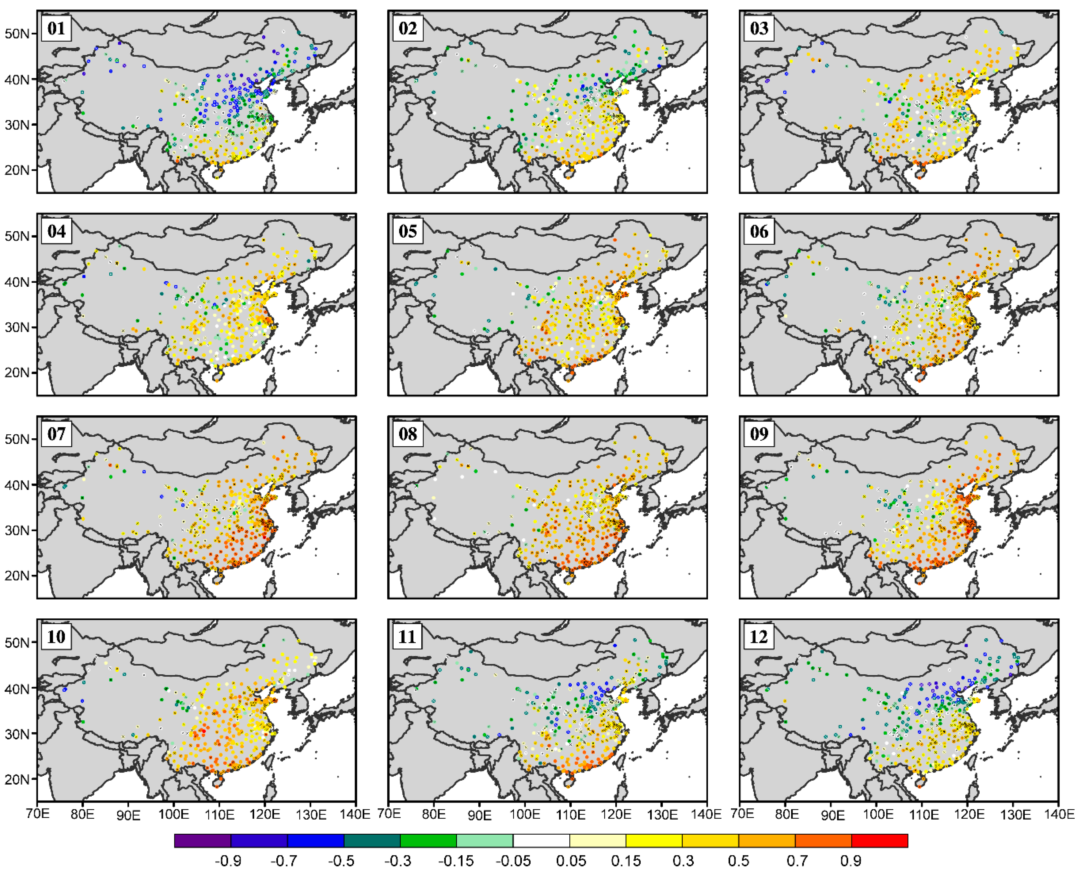
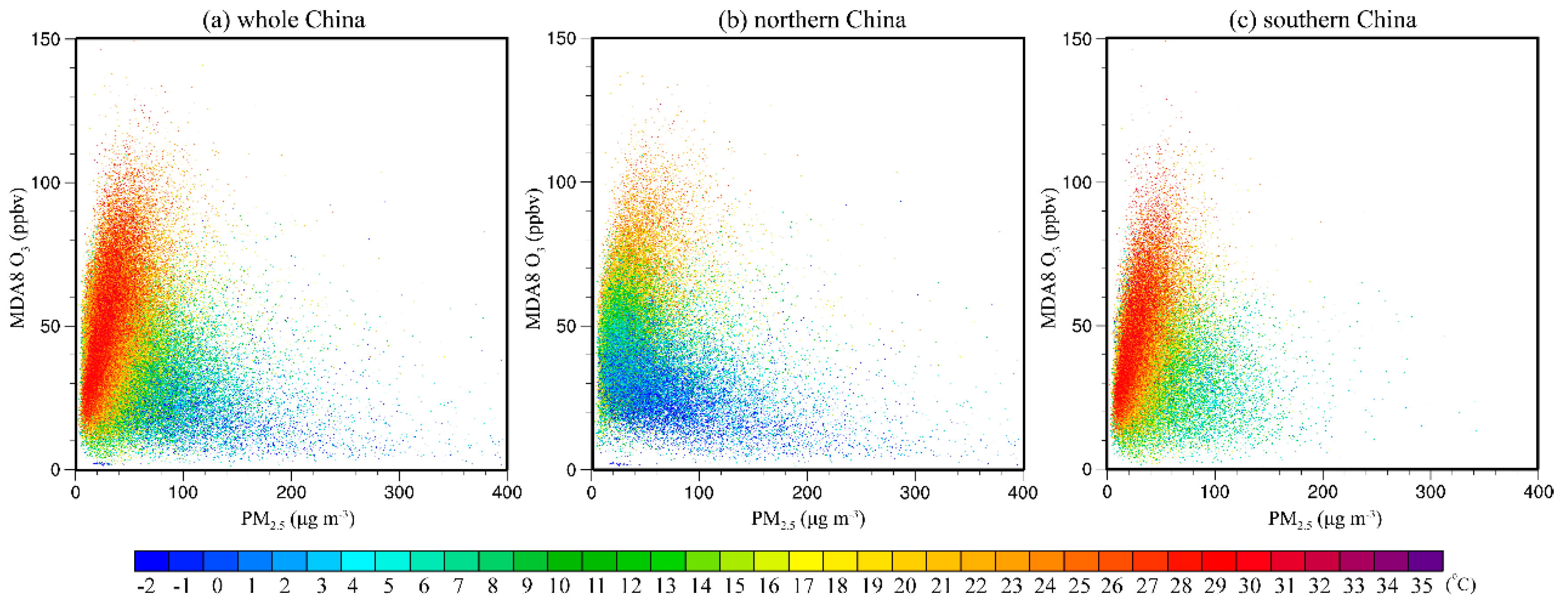
3.1. Observed PM2.5–O3 Correlations

Figure 1 shows the spatial-temporal distributions of correlations between daily PM2.5 and MDA8 O3 concentrations over China. Each panel represents each month for the year 2016. It is too intensive to display all 1497 sites on the map, therefore, we present the correlations for all 360 cities. The PM2.5 concentrations were positively correlated with O3 concentrations for most regions and seasons over China, while the negative correlations mainly existed in northern China during winter. The strongest positive correlations (r > +0.7) were observed in southern China during July, and the strongest negative correlations (r < −0.5) were observed in northern China during January, with most cities passing the 95% confidence level.
Interestingly, the spatial-temporal distributions of PM2.5–O3 correlations highly resembled those of temperature (shown in Figure S1). Both the PM2.5–O3 correlations and temperature reached the maximum in southern China during July and reached the minimum in northern China during January. To further investigate the relations between PM2.5–O3 correlations and temperature, we provide scatter plots of daily PM2.5 and MDA8 O3 concentrations color coded with temperature for all cities of the whole China during 2016 in Figure 2a. Regularly, a positive correlation between PM2.5 and O3 was found for high air temperature samples, while a negative correlation prevailed in cold environments. The phenomenon can be presented more clearly when the data points are separated into northern cities (shown in Figure 2b) and southern cities (shown in Figure 2c). A remarkable positive correlation was found for high temperature over southern China and a significant negative correlation was observed for low temperature over northern China, which was also well reflected in Figure 1. It was noted that the relations between PM2.5–O3 correlations and other meteorological parameters (e.g., relative humidity) were much weaker (scatter plots for other meteorological parameters were not shown).
In the following sections, we focus on comparing data points which exhibit the strongest positive PM2.5–O3 correlations and high air temperature (i.e., southern China in July) and those that exhibit the strongest negative PM2.5–O3 correlations and low air temperature (i.e., northern China in January), to investigate the underlying reasons for the varying PM2.5–O3 correlations.

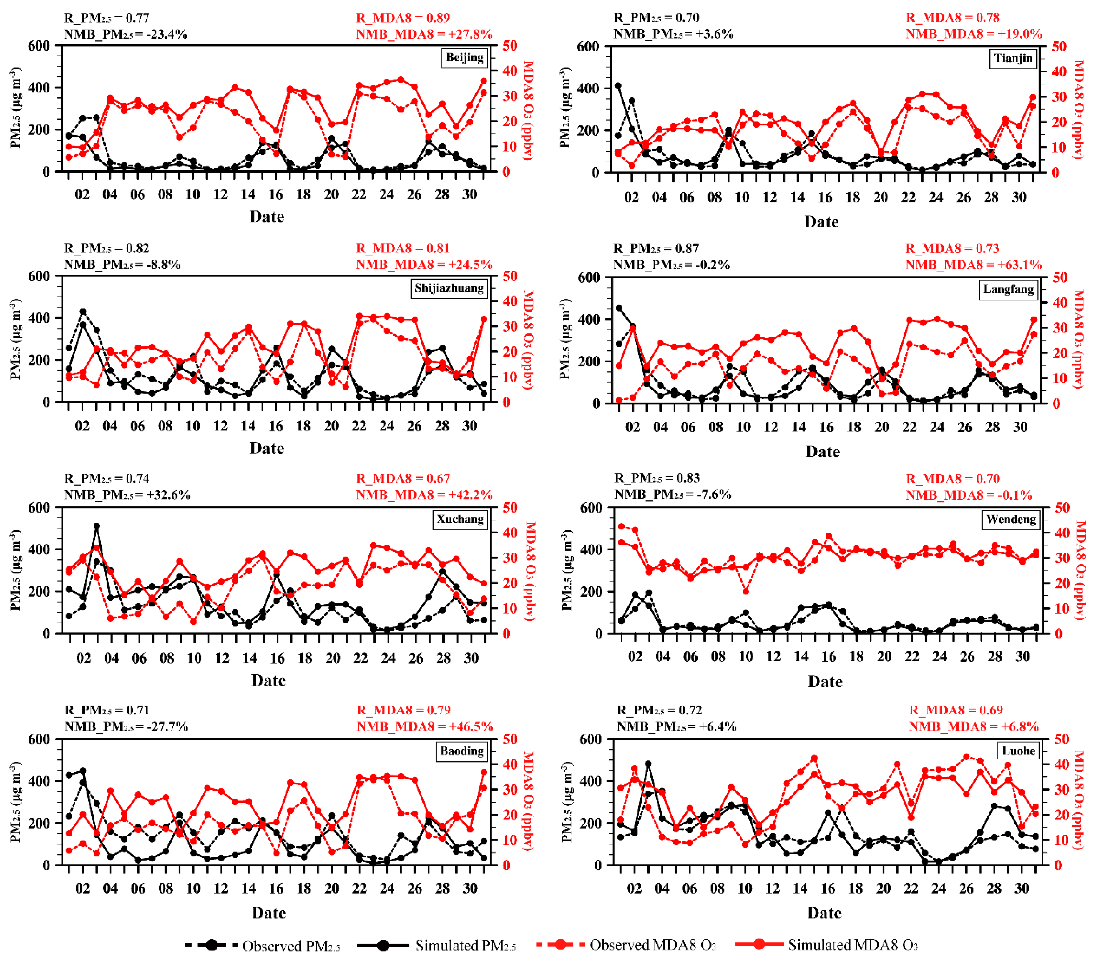
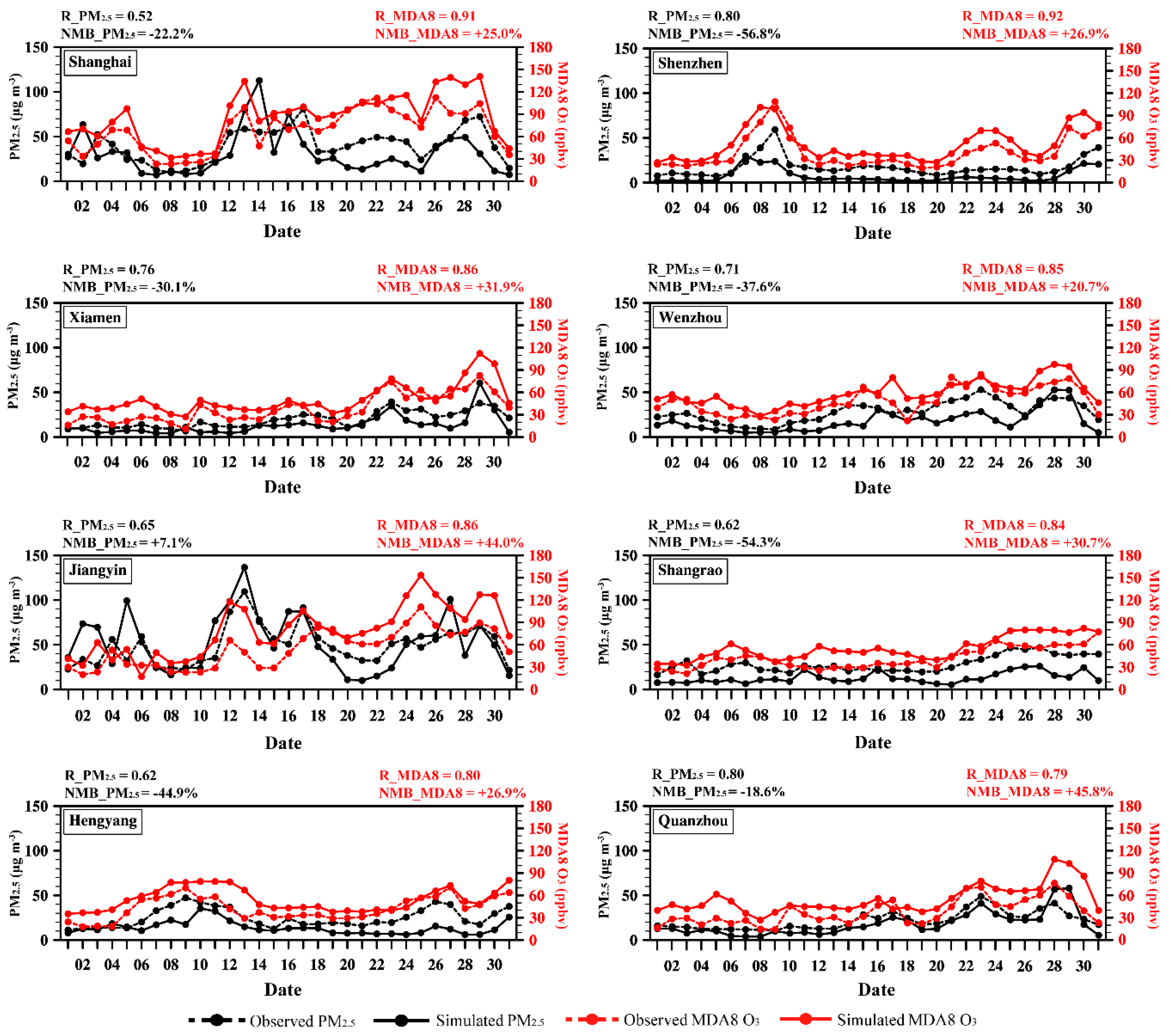
3.2. Model Evaluation

Previous studies have indicated that the GEOS-Chem model captures the distributions of observed PM2.5 [13,48,49] and O3 [11,50,51,52] over China fairly well. We conducted comparisons with the MEE measurements here to evaluate whether the version of the GEOS-Chem model used in this study can reproduce the observed variations in surface-layer PM2.5 and O3 and their correlations.
The observed and simulated daily PM2.5 and MDA8 O3 concentrations for northern cities in January and southern cities in July are shown in Figure 3 and Figure 4, respectively. Although the model generally underestimated (overestimated) the absolute PM2.5 (MDA8 O3) concentrations, the model successfully captured the temporal variations of PM2.5 and MDA8 O3 concentrations. For northern cities in January, the correlation coefficients between the simulated and observed PM2.5 (MDA8 O3) concentrations ranged from 0.70 to 0.87 (from 0.67 to 0.89); for southern cities in July, the correlation coefficients for PM2.5 (MDA8 O3) were in the range of 0.52 to 0.80 (0.79 to 0.92). For both observed and simulated concentrations, PM2.5 presented an overall negative correlation with MDA8 O3 in northern China during January but exhibited a significant positive correlation with MDA8 O3 in southern China during July. The observed inverse correlations were reproduced by the GEOS-Chem model fairly well. Therefore, it was feasible to conduct PM2.5–O3 correlation analysis using the GEOS-Chem model.

3.3. Underlying Reasons and Mechanisms

As mentioned in the Introduction, there exist interactions between PM2.5 and O3. However, PM2.5 and O3 may exhibit varying and even inverse correlations in different seasons and different regions, which indicates that the importance of different interactions on the PM2.5–O3 correlations may vary over time across space. The Beijing–Tianjin–Hebei (BTH, 37°–41° N, 114°–118° E) agglomeration, as the representative of northern China, has a low temperature below 0 °C and the strongest negative PM2.5–O3 correlation in January. The Pearl River Delta (PRD, 22°–24° N, 112°–115° E) agglomeration, as the representative of southern China, has a high temperature above 27 °C and the strongest positive PM2.5–O3 correlation in July. Therefore, in this section, we chose the BTH in January (as the representative of negative PM2.5–O3 correlations and low temperature) and PRD in July (as the representative of positive PM2.5–O3 correlations and high temperature), to compare the importance of different PM2.5–O3 interactions on the correlations for different regions and seasons (i.e., different temperature) and reveal the underlying reasons/mechanisms, based on the GEOS-Chem simulation.

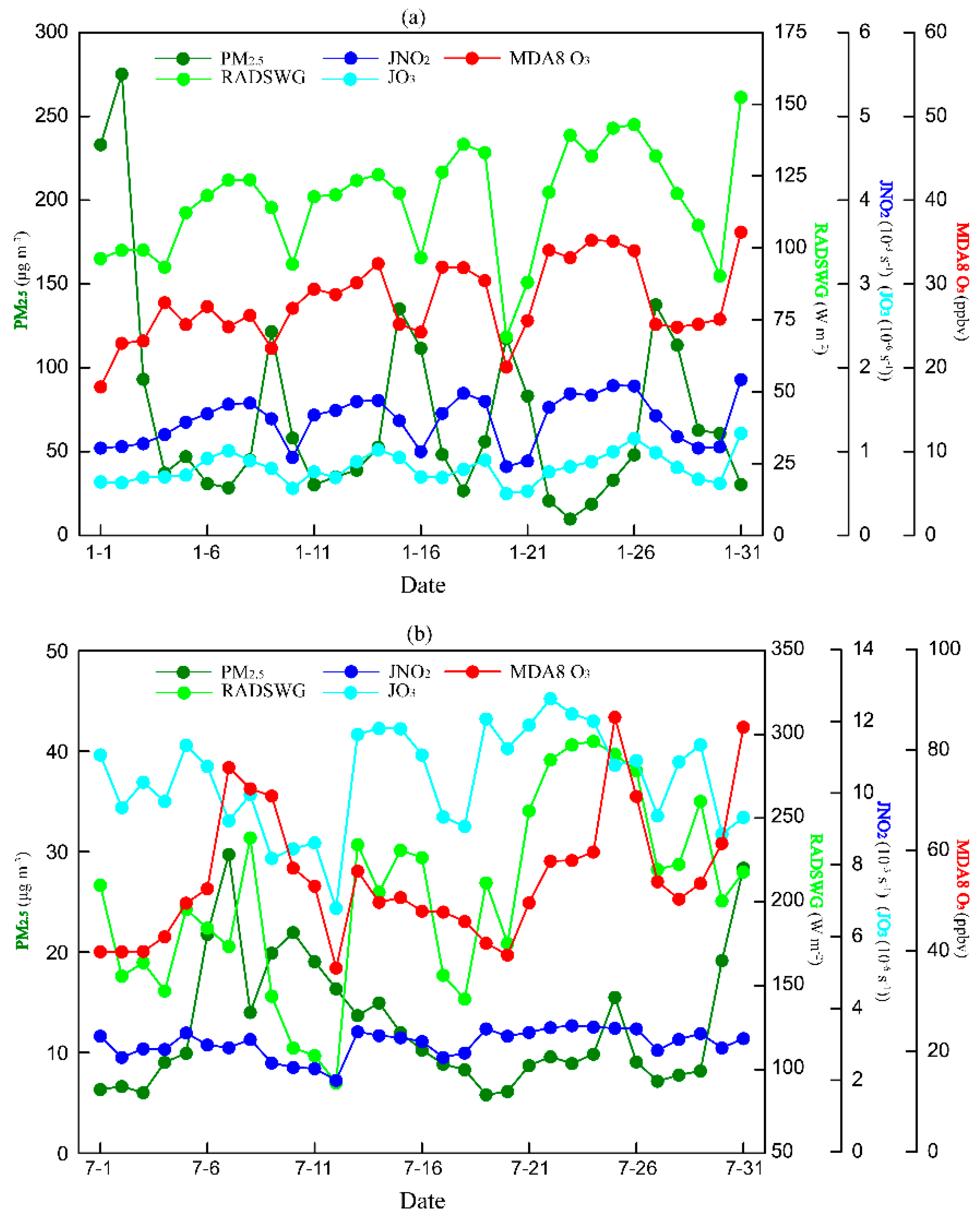
3.3.1. PM2.5 Suppressing O3 Generation by Reducing Photolysis Rates

Particulates may decrease the actinic flux of incident solar radiation by scattering or absorbing solar radiation directly and altering the optical properties of clouds indirectly, and inhibit the photolysis reactions near the surface by reducing the photolysis rates, which finally reduce the O3 generation [26,27,28,29,30,31].
Figure 5 shows the time-series of simulated daily PM2.5 concentrations, solar radiation at the ground (RADSWG), photolysis rates (J(NO2) and J(O3)), and MDA8 O3 concentrations, for BTH in January and PRD in July. It is remarkable in Figure 5a that the RADSWG was negatively correlated with PM2.5 (r = −0.45), indicating the strong extinction effects of particulates on solar radiation. The photolysis rates, including J(NO2) and J(O3), and MDA8 O3 concentrations presented significantly positive correlation with RADSWG, which finally resulted in a strongly negative correlation between PM2.5 and MDA8 O3 for BTH in January. Influenced by meteorological conditions, the PM2.5 concentrations exhibited spikes and valleys. When the PM2.5 concentrations reached the peaks, the RADSWG, photolysis rates, and MDA8 O3 concentrations reached the lowest levels due to the inhibitory effect of PM2.5 on O3 generation by reducing photolysis rates. By contrast, for PRD in July (Figure 5b), the correlation between RADSWG and PM2.5 was much smaller (r = −0.27), indicating a weaker extinction effect of particulates on solar radiation and a consequently weaker influence on photolysis rates and MDA8 O3 concentrations. For BTH in January, the average PM2.5 concentrations were relatively high because of winter heating and low boundary layer height associated with low temperature, which led to a more effective suppressing effect of PM2.5 on O3 generation by reducing photolysis rates for cold environments. A similar phenomenon has also been reported by Tie et al. [26], who pointed out that surface photolysis rates J(NO2) and J(O3) in Eastern China were reduced by 10–30% and 20–30% due to the effect of particulates on photolytic radiation in winter, as well as 1–10% and 5–20% in summer, leading to reductions in surface O3 concentrations by 2–4% in winter and less than 2% in summer. Overall, the negative PM2.5–O3 correlation for cold environment may be partly attributed to the effective inhibitory effect of PM2.5 on O3 generation by reducing photolysis rates at low temperature.

3.3.2. NO Suppressing O3 Production through the NO Titration Effect

It is known that excessive NO is not favorable for O3 generation. If NO levels are high, O3 production is suppressed by the “ O 3 + NO NO 2 + O 2 ” reaction, usually referred to as NO titration, which is an important O3 removal process associated with freshly emitted NO [14,53].
The time-series of simulated daily PM2.5, BC, NO, and MDA8 O3 concentrations, for BTH in January and PRD in July, are shown in Figure 6. The NO concentration was calculated to be 8.5 ppbv averaged over BTH in January, six times that for PRD in July. It is conspicuous, in Figure 6a, that the MDA8 O3 was negatively correlated with NO with a high correlation coefficient of −0.74, indicating a strong NO titration effect for BTH in January. When the NO concentrations reached the spikes, the MDA8 O3 concentrations reached the valleys due to the strong NO titration effect. By contrast, the NO titration effect for PRD in July was weaker; the correlation coefficient between MDA8 O3 and NO was −0.55. Ding et al. [20] and Chen et al. [25] also reported similar finding that the negative correlation mainly existed for low temperature data, suggesting a titration effect of freshly emitted NO with O3 in cold seasons.
For BTH in January, the lower air temperature (generally indicating the feebler solar radiation) resulted in weaker atmospheric oxidation ability, therefore, more NO was freshly emitted. The BC, as a primary particulate, was difficult to generate or clear through chemical reactions. It is noted that NO and BC, as well as PM2.5, have similar sources, such as combustion and traffic activities [20,25]. Therefore, the freshly emitted NO presented a significant positive correlation with the primary particulate BC (r = 0.85) and consequently with PM2.5 (r = 0.73). In contrast, for PRD in July, more NO was converted to NO2, and therefore, NO tended to be less correlated with the primary particulate BC (r = 0.39) and consequently with PM2.5 (r = −0.13) (Figure 6b).
In conclusion, the significant negative correlation between NO and MDA8 O3, and the remarkable positive correlation between NO and PM2.5, led to the negative correlation between PM2.5 and MDA8 O3 for BTH in January. The negative PM2.5–O3 correlation at low temperature may be partly attributed to the strong titration effect of high NO concentration, which is consistent with primary PM2.5 in a cold environment.

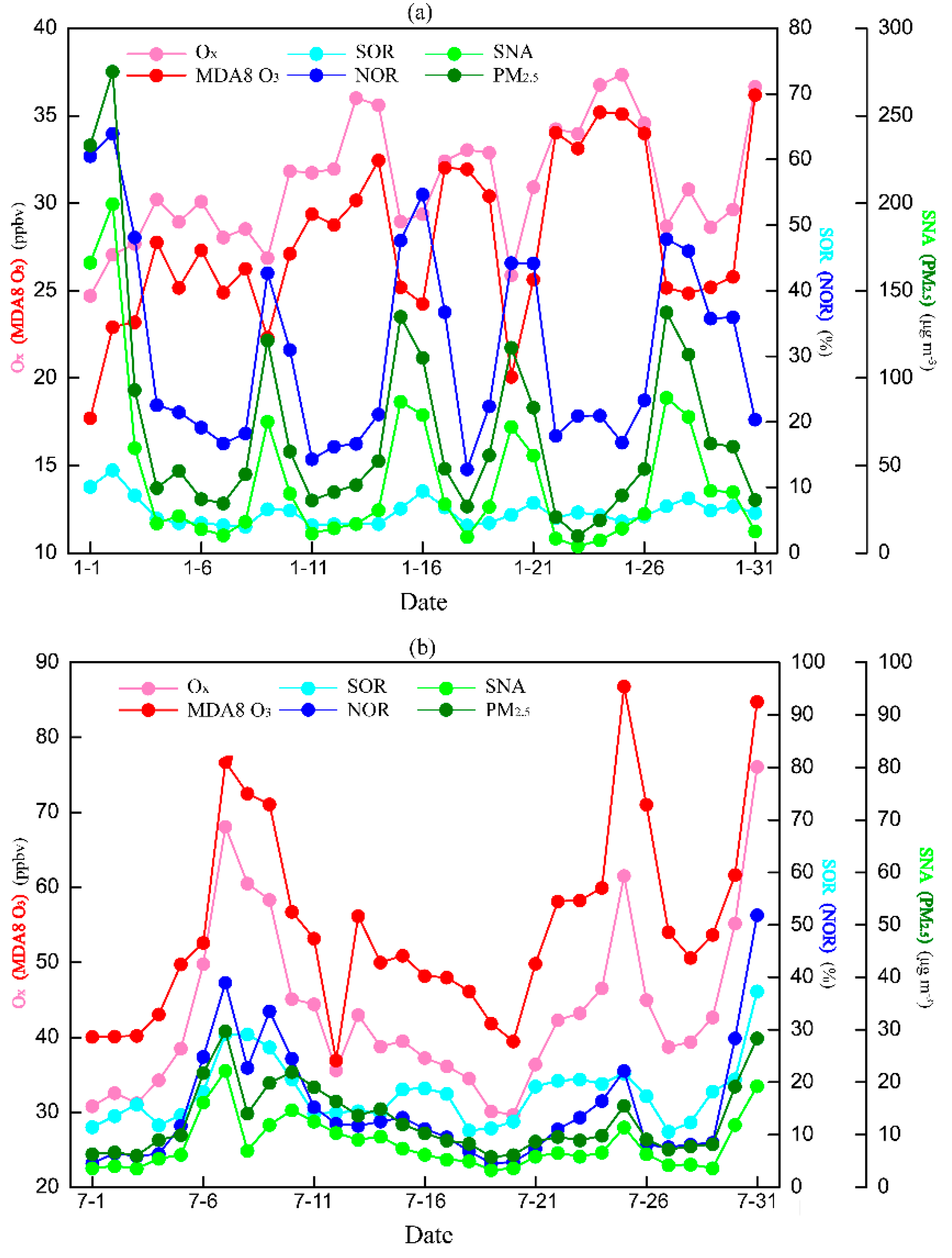
3.3.3. High O3 Concentration and Active Photochemical Activity Promoting Secondary PM2.5 Formation

As reported in previous studies, high O3 concentration generally indicates strong atmospheric photochemical reactivity, which can promote the secondary particulate formation. For example, the photochemical oxidation of SO2 to H2SO4 may be promoted by strong atmospheric photochemical reactions, and the formation of HNO3 can be strongly enhanced by high O3 [19,32].
To examine the effects of O3 and photochemical activity on secondary particulate formation under different temperature conditions, we compared the time-series of simulated daily Ox and MDA8 O3 concentrations, SOR and NOR, as well as SNA and PM2.5 concentrations between BTH in January and PRD in July in Figure 7. The total oxidant Ox (Ox = O3 + NO2) was used to characterize the atmospheric oxidation capacity, following Wang et al. [14], Jia et al. [22], and Clapp and Jenkin [54]. The sulfur oxidation ratio, SOR = n-SO42−/(n-SO42− + n-SO2), was a measure of the conversion degree of sulfur; the nitrogen oxidation ratio, which was defined as NOR = n-NO3/(n-NO3 + n-NO2), was used to quantitatively express the conversion degree of nitrogen [55,56,57,58]. The secondary inorganic particulate was defined as SNA = SO42− + NO3 + NH4+.
For PRD in July (Figure 7b), the correlation coefficient between MDA8 O3 and Ox was 0.93, indicating the important role of O3 on the atmospheric oxidizing capacity. The SOR (NOR) exhibited a pronounced positive correlation with Ox, with a high correlation coefficient of 0.89 (0.93), which indicates that the formation of secondary inorganic particulates can be promoted by photochemical oxidation and O3. Consequently, the SNA and PM2.5 were positively correlated with Ox and MDA8 O3 concentrations. It is noted that high concentrations of O3 and strong atmospheric photochemical reactions may also enhance the formation of secondary organic aerosol (SOA) [19]. By analyzing concentrations of SOA and gas pollutants measured in the summer of 2013, Wang et al. [19] found that SOA had a good correlation with Ox, with a correlation coefficient of 0.90, which indicated that SOA formation was mainly promoted by photochemical oxidation. In contrast, the correlation between SOR (NOR) and Ox was much smaller and even negative for BTH in January (Figure 7a). In general, high air temperature means strong solar radiation and high O3 concentration. Therefore, the promoting effect of high O3 concentration and active photochemical activity on secondary PM2.5 formation was more effective under high temperature conditions.
Overall, in an environment of high temperature, high concentration of O3 indicates a strong atmospheric photochemical reactivity, and significantly promotes the level of atmospheric oxidation. The strong atmospheric oxidation capacity, in turn, enhances the formation of both secondary inorganic particulates and secondary organic particulates. The enhanced formation of secondary particulates eventually leads to significant positive PM2.5–O3 correlation in a hot environment.

4. Conclusions and Discussion

In this study, the spatial-temporal characteristics of the correlations between PM2.5 and O3 were investigated at the national-scale level, based on the pollutant concentrations measured at all monitoring sites in China from the Ministry of Ecological and Environment for the whole year of 2016. The underlying reasons or mechanisms on the varying PM2.5–O3 correlations in different regions and seasons were examined by a chemical transport model (GEOS–Chem).
Measurements showed that the PM2.5 concentrations were positively correlated with O3 concentrations for most regions and seasons over China, while the negative correlations were mainly observed in northern China during winter. The strongest positive PM2.5–O3 correlations with correlation coefficients (r) larger than +0.7 existed in southern China during July, and the strongest negative correlations (r < −0.5) were observed in northern China during January.
It was very interesting to see that the spatial-temporal distributions of PM2.5–O3 correlations highly resembled those of temperature. Therefore, the relations between PM2.5–O3 correlations and temperature were further investigated. Regularly, the positive PM2.5–O3 correlations prevailed for high air temperature samples, while the negative correlations were generally found in a cold environment.
We then focused on comparing data points which exhibited the strongest positive PM2.5–O3 correlations and high air temperature (i.e., southern China in July) and those that exhibited the strongest negative PM2.5–O3 correlations and low air temperature (i.e., northern China in January) to investigate the underlying reasons for the varying PM2.5–O3 correlations for different regions and seasons (i.e., different temperature), based on the GEOS-Chem simulation. Model evaluations showed that it was viable and reliable to conduct PM2.5–O3 correlation analysis using the GEOS-Chem model.
The PM2.5 may suppress O3 generation by reducing photolysis rates. For northern China in January (i.e., low temperature condition), the average PM2.5 concentrations were relatively high, which led to a more effective inhibitory effect of PM2.5 on O3 generation for cold environments than for hot environments. Therefore, the negative PM2.5–O3 correlation for a cold environment may be partly attributed to the effective inhibitory effect of PM2.5 on O3 generation by reducing photolysis rates at low temperature. The NO may suppress O3 production through the NO titration effect, and the inhibitory effect was found to be stronger for low temperature conditions than for high temperature conditions. However, the freshly emitted NO presented a significant positive correlation with the primary particulate BC, and consequently, with PM2.5 in cold seasons. Therefore, the negative PM2.5–O3 correlation at low temperature may also be partly attributed to the strong titration effect of high NO concentration, which was consistent with primary PM2.5 in a cold environment. High concentration of O3 generally indicates active photochemical activity, which may promote the secondary PM2.5 formation. In general, high O3 concentration occurs in an environment of high temperature and strong solar radiation. Therefore, the positive PM2.5–O3 correlation in a hot environment may be a result of the promoting effect of high O3 concentration and active photochemical activity on secondary particle formation.
In conclusion, the effective inhibitory effect of PM2.5 on O3 generation by reducing photolysis rates at low temperature, and the strong titration effect of freshly emitted NO with O3 in cold seasons, together contribute to the strongest negative PM2.5–O3 correlation in cold environments. The strongest positive PM2.5–O3 correlation at high temperature, however, is mainly attributed to the promoting effect of high O3 concentration and active photochemical activity on secondary particle formation in hot environments.
This paper revealed three underlying reasons for the PM2.5–O3 correlations. It is noted that heterogeneous chemical reaction is an important way for PM2.5–O3 interaction [17,59,60,61,62], which may also be a reason for the PM2.5–O3 correlations. The formation of SOA with high O3 concentration may contribute to positive correlations, because biogenic emission of VOCs is high under high temperature conditions in summer [20,25]. Furthermore, the variations in meteorological variables, through affecting transport and chemical processes of pollutants, may be important for daily variations in PM2.5 and O3, and therefore, contribute to the PM2.5–O3 correlations. Comprehensively understanding all these chemical and physical mechanisms needs more in-depth research through sensitivity experiments in future studies.

Supplementary Materials

The following are available online at https://www.mdpi.com/2073-4433/10/7/352/s1, Figure S1: Spatial-temporal distributions of surface temperature (℃). Each panel represents each month for year 2016.

Author Contributions

Conceptualization, J.Z. and H.L.; Formal analysis, J.Z. and L.C.; Funding acquisition, J.Z. and H.L.; Investigation, J.Z. and R.D.; Methodology, J.Z.; Software, L.C.; Validation, R.D.; Visualization, L.C.; Writing—original draft, J.Z.; Writing—review and editing, H.L.

Funding

This research was funded by the University Natural Science Research Foundation of Jiangsu Province: 18KJB170012, the Startup Foundation for Introducing Talent of NUIST: 2018r007, the National Natural Science Foundation of China: 91744311, and the Postgraduate Research and Practice Innovation Program of Jiangsu Province: KYCX18_1018.

Acknowledgments

This study was supported by the University Natural Science Research Foundation of Jiangsu Province (18KJB170012), the Startup Foundation for Introducing Talent of NUIST (2018r007), the National Natural Science Foundation of China (91744311), and the Postgraduate Research and Practice Innovation Program of Jiangsu Province (KYCX18_1018). The authors acknowledge the free use of monitoring air quality data provided by the Ministry of Ecological and Environment (MEE) and the meteorological data of surface temperature provided by the European Centre for Medium-Range Weather Forecasts (ECMWF). We also appreciate the anonymous reviewers for their constructive comments and thoughtful suggestions.

Conflicts of Interest

The authors declare no conflict of interest.

References

  1. Maji, K.J.; Dikshit, A.K.; Arora, M.; Deshpande, A. Estimating premature mortality attributable to PM2.5 exposure and benefit of air pollution control policies in China for 2020. Sci. Total Environ. 2018, 612, 683–693. [Google Scholar] [CrossRef] [PubMed]
  2. Wang, Q.; Wang, J.; He, M.Z.; Kinney, P.L.; Li, T. A county-level estimate of PM2.5 related chronic mortality risk in china based on multi-model exposure data. Env. Int. 2018, 110, 105–112. [Google Scholar] [CrossRef] [PubMed]
  3. Jeensorn, T.; Apichartwiwat, P.; Jinsart, W. PM10 and PM2.5 from haze smog and visibility effect in Chiang Mai Province, Thailand. App. Envi. Res. 2018, 40, 1–10. [Google Scholar]
  4. Li, Y.C.; Shu, M.; Ho, S.S.H.; Yu, J.-Z.; Yuan, Z.-B.; Wang, X.-X.; Zhao, X.-Q.; Liu, Z.-F. Effects of chemical composition of PM2.5 on visibility in a semi-rural city of sichuan basin. Aerosol Air Qual. Res. 2018, 18, 957–968. [Google Scholar] [CrossRef]
  5. Yang, C.; Yang, H.; Guo, S.; Wang, Z.; Xu, X.; Duan, X.; Kan, H. Alternative ozone metrics and daily mortality in Suzhou: The China air pollution and health effects study (CAPES). Sci. Total Env. 2012, 426, 83–89. [Google Scholar] [CrossRef] [PubMed]
  6. Tai, A.P.K.; Martin, M.V.; Heald, C.L. Threat to future global food security from climate change and ozone air pollution. Nat. Clim. Chang. 2014, 4, 817–821. [Google Scholar] [CrossRef] [Green Version]
  7. Yue, X.; Unger, N. Ozone vegetation damage effects on gross primary productivity in the United States. Atmos. Chem. Phys. 2014, 14, 9137–9153. [Google Scholar] [CrossRef] [Green Version]
  8. Raza, A.; Dahlquist, M.; Lind, T.; Ljungman, P.L.S. Susceptibility to short-term ozone exposure and cardiovascular and respiratory mortality by previous hospitalizations. Env. Health 2018, 17, 37. [Google Scholar] [CrossRef] [Green Version]
  9. Gao, Y.; Zhang, M. Sensitivity analysis of surface ozone to emission controls in Beijing and its neighboring area during the 2008 Olympic Games. J. Env. Sci. 2012, 24, 50–61. [Google Scholar] [CrossRef]
  10. Gao, Y.; Zhang, M.; Liu, Z.; Wang, L.; Wang, P.; Xia, X.; Tao, M.; Zhu, L. Modeling the feedback between aerosol and meteorological variables in the atmospheric boundary layer during a severe fog–haze event over the North China Plain. Atmos. Chem. Phys. 2015, 15, 4279–4295. [Google Scholar] [CrossRef]
  11. Wang, Y.; Zhang, Y.; Hao, J.; Luo, M. Seasonal and spatial variability of surface ozone over China: Contributions from background and domestic pollution. Atmos. Chem. Phys. 2011, 11, 3511–3525. [Google Scholar] [CrossRef]
  12. Li, K.; Jacob, D.J.; Liao, H.; Shen, L.; Zhang, Q.; Bates, K.H. Anthropogenic drivers of 2013–2017 trends in summer surface ozone in China. Proc. Natl. Acad. Sci. USA 2019, 116, 422–427. [Google Scholar] [CrossRef] [PubMed]
  13. Li, K.; Liao, H.; Zhu, J.; Moch, J.M. Implications of RCP emissions on future PM2.5 air quality and direct radiative forcing over China. J. Geophys. Res. Atmos. 2016, 121, 12985–13008. [Google Scholar] [CrossRef]
  14. Wang, T.; Xue, L.; Brimblecombe, P.; Lam, Y.F.; Li, L.; Zhang, L. Ozone pollution in china: A review of concentrations, meteorological influences, chemical precursors, and effects. Sci. Total Env. 2017, 575, 1582–1596. [Google Scholar] [CrossRef] [PubMed]
  15. Tao, M.; Chen, L.; Wang, Z.; Wang, J.; Tao, J.; Wang, X. Did the widespread haze pollution over China increase during the last decade? A satellite view from space. Env. Res. Lett. 2016, 11, 054019. [Google Scholar] [CrossRef]
  16. Tao, M.; Chen, L.; Xiong, X.; Zhang, M.; Ma, P.; Tao, J.; Wang, Z. Formation process of the widespread extreme haze pollution over northern China in January 2013: Implications for regional air quality and climate. Atmos. Env. 2014, 98, 417–425. [Google Scholar] [CrossRef]
  17. Stadtler, S.; Simpson, D.; Schröder, S.; Taraborrelli, D.; Bott, A.; Schultz, M. Ozone impacts of gas–aerosol uptake in global chemistry transport models. Atmos. Chem. Phys. 2018, 18, 3147–3171. [Google Scholar] [CrossRef]
  18. Pathak, R.K.; Wu, W.S.; Wang, T. Summertime PM2.5 ionic species in four major cities of China: Nitrate formation in an ammonia-deficient atmosphere. Atmos. Chem. Phys. 2009, 9, 1711–1722. [Google Scholar] [CrossRef]
  19. Wang, D.; Zhou, B.; Fu, Q.; Zhao, Q.; Zhang, Q.; Chen, J.; Yang, X.; Duan, Y.; Li, J. Intense secondary aerosol formation due to strong atmospheric photochemical reactions in summer: Observations at a rural site in eastern Yangtze River Delta of China. Sci. Total Env. 2016, 571, 1454–1466. [Google Scholar] [CrossRef]
  20. Ding, A.J.; Fu, C.B.; Yang, X.Q.; Sun, J.N.; Zheng, L.F.; Xie, Y.N.; Herrmann, E.; Nie, W.; Petäjä, T.; Kerminen, V.M.; et al. Ozone and fine particle in the western Yangtze River Delta: An overview of 1 yr data at the SORPES station. Atmos. Chem. Phys. 2013, 13, 5813–5830. [Google Scholar] [CrossRef]
  21. Wang, Y.; Ying, Q.; Hu, J.; Zhang, H. Spatial and temporal variations of six criteria air pollutants in 31 provincial capital cities in China during 2013–2014. Env. Int. 2014, 73, 413–422. [Google Scholar] [CrossRef]
  22. Jia, M.; Zhao, T.; Cheng, X.; Gong, S.; Zhang, X.; Tang, L.; Liu, D.; Wu, X.; Wang, L.; Chen, Y. Inverse relations of PM2.5 and O3 in air compound pollution between cold and hot seasons over an urban area of east China. Atmosphere 2017, 8, 59. [Google Scholar] [CrossRef]
  23. Tang, B.Y.; Xin, J.Y.; Gao, W.K.; Shao, P.; Su, H.J.; Wen, T.X.; Song, T.; Fan, G.Z.; Wang, S.G.; Wang, Y.S. Characteristics of complex air pollution in typical cities of North China. Atmos. Ocean. Sci. Lett. 2018, 11, 29–36. [Google Scholar] [CrossRef]
  24. Zhao, H.; Zheng, Y.; Li, C. spatiotemporal distribution of PM2.5 and O3 and their interaction during the summer and winter seasons in Beijing, China. Sustainability 2018, 10, 4519. [Google Scholar] [CrossRef]
  25. Chen, H.; Zhuang, B.; Liu, J.; Wang, T.; Li, S.; Xie, M.; Li, M.; Chen, P.; Zhao, M. Characteristics of ozone and particles in the near-surface atmosphere in the urban area of the Yangtze River Delta, China. Atmos. Chem. Phys. 2019, 19, 4153–4175. [Google Scholar] [CrossRef] [Green Version]
  26. Tie, X.X.; Madronich, S.; Walters, S.; Edwards, D.P.; Ginoux, P.; Mahowald, N.; Zhang, R.Y.; Lou, C.; Brasseur, G. Assessment of the global impact of aerosols on tropospheric oxidants. J. Geophys. Res. 2005, 110, D03204. [Google Scholar] [CrossRef]
  27. Menon, S.; Unger, N.; Koch, D.; Francis, J.; Garrett, T.; Sednev, I.; Shindell, D.; Streets, D. Aerosol climate effects and air quality impacts from 1980 to 2030. Env. Res. Lett. 2008, 3, 024004. [Google Scholar] [CrossRef]
  28. Unger, N.; Menon, S.; Koch, D.M.; Shindell, D.T. Impacts of aeroso-cloud interaction on past and future changes in tropospheric composition. Atmos. Chem. Phys. 2009, 9, 4115–4130. [Google Scholar] [CrossRef]
  29. Li, J.; Wang, Z.; Wang, X.; Yamaji, K.; Takigawa, M.; Kanaya, Y.; Pochanart, P.; Liu, Y.; Irie, H.; Hu, B.; et al. Impacts of aerosols on summertime tropospheric photolysis frequencies and photochemistry over Central Eastern China. Atmos. Env. 2011, 45, 1817–1829. [Google Scholar] [CrossRef]
  30. Li, M.; Wang, T.; Xie, M.; Li, S.; Zhuang, B.; Chen, P.; Huang, X.; Han, Y. Agricultural fire impacts on ozone photochemistry over the Yangtze River Delta region, East China. J. Geophys. Res.-Atmos. 2018, 123, 6605–6623. [Google Scholar] [CrossRef]
  31. Real, E.; Sartelet, K. Modeling of photolysis rates over Europe: Impact on chemical gaseous species and aerosols. Atmos. Chem. Phys. 2011, 11, 1711–1727. [Google Scholar] [CrossRef]
  32. Khoder, M.I. Atmospheric conversion of sulfur dioxide to particulate sulfate and nitrogen dioxide to particulate nitrate and gaseous nitric acid in an urban area. Chemosphere 2002, 49, 675–684. [Google Scholar] [CrossRef]
  33. Chang, S.C.; Lee, C.T. Secondary aerosol formation through photochemical reactions estimated by using air quality monitoring data in Taipei City from 1994 to 2003. Atmos. Env. 2007, 41, 4002–4017. [Google Scholar] [CrossRef]
  34. Li, L.; Chen, C.H.; Huang, C.; Huang, H.Y.; Zhang, G.F.; Wang, Y.J.; Wang, H.L.; Lou, S.R.; Qiao, L.P.; Zhou, M.; et al. Process analysis of regional ozone formation over the Yangtze River Delta, China using the Community Multi-scale Air Quality modeling system. Atmos. Chem. Phys. 2012, 12, 10971–10987. [Google Scholar] [CrossRef] [Green Version]
  35. Seinfeld, J.H.; Pandis, S.N. Atmospheric Chemistry and Physics: From Air Pollution to Climate Change, 3rd ed.; John Wiley & Sons, Inc.: Hoboken, NJ, USA, 2016. [Google Scholar]
  36. Xu, X.; Shi, X.; Xie, L.; Ding, G.; Miao, Q.; Ma, J.; Zheng, X. Spatial characteristics of urban gaseous and particulate pollutants in winter and summer. Sci. China Ser. D 2005, 35, 53–65. [Google Scholar] [CrossRef]
  37. Xiao, Z.M.; Zhang, Y.F.; Hong, S.M.; Bi, X.H.; Jiao, L.; Feng, Y.C.; Wang, Y.Q. Estimation of the main factors influencing haze, based on a long-term monitoring campaign in Hangzhou, China. Aerosol Air Qual. Res. 2011, 11, 873–882. [Google Scholar] [CrossRef]
  38. Shi, C.; Wang, S.; Liu, R.; Zhou, R.; Li, D.; Wang, W.; Li, Z.; Cheng, T.; Zhou, B. A study of aerosol optical properties during ozone pollution episodes in 2013 over Shanghai, China. Atmos. Res. 2015, 153, 235–249. [Google Scholar] [CrossRef]
  39. Zhang, Y.Y.; Jia, Y.; Li, M.; Hou, L.A. Spatiotemporal variations and relationship of PM and gaseous pollutants based on gray correlation analysis. J. Env. Sci. Health A Tox. Hazard. Subst. Env. Eng. 2018, 53, 139–145. [Google Scholar] [CrossRef]
  40. Dee, D.P.; Uppala, S.M.; Simmons, A.J.; Berrisford, P.; Poli, P.; Kobayashi, S.; Andrae, U.; Balmaseda, M.A.; Balsamo, G.; Bauer, P.; et al. The ERA-Interim reanalysis: Configuration and performance of the data assimilation system. Q. J. Roy. Meteor. Soc. 2011, 137, 553–597. [Google Scholar] [CrossRef]
  41. Wang, X.; Dickinson, R.E.; Su, L.; Zhou, C.; Wang, K. PM2.5 pollution in China and how it has been exacerbated by terrain and meteorological conditions. B. Am. Meteorol. Soc. 2018, 99, 105–119. [Google Scholar] [CrossRef]
  42. Zhong, J.; Zhang, X.; Wang, Y.; Wang, J.; Shen, X.; Zhang, H.; Wang, T.; Xie, Z.; Liu, C.; Zhang, H.; et al. The two-way feedback mechanism between unfavorable meteorological conditions and cumulative aerosol pollution in various haze regions of China. Atmos. Chem. Phys. 2019, 19, 3287–3306. [Google Scholar] [CrossRef] [Green Version]
  43. Travis, K.R.; Jacob, D.J.; Fisher, J.A.; Kim, P.S.; Marais, E.A.; Zhu, L.; Yu, K.; Miller, C.C.; Yantosca, R.M.; Sulprizio, M.P.; et al. Why do models overestimate surface ozone in the Southeast United States? Atmos. Chem. Phys. 2016, 16, 13561–13577. [Google Scholar] [CrossRef] [PubMed] [Green Version]
  44. Gelaro, R.; McCarty, W.; Suárez, M.J.; Todling, R.; Molod, A.; Takacs, L.; Randles, C.A.; Darmenov, A.; Bosilovich, M.G.; Reichle, R.; et al. The modern-era retrospective analysis for research and applications, version 2 (MERRA-2). J. Clim. 2017, 30, 5419–5454. [Google Scholar] [CrossRef]
  45. Li, M.; Zhang, Q.; Kurokawa, J.-I.; Woo, J.-H.; He, K.; Lu, Z.; Ohara, T.; Song, Y.; Streets, D.G.; Carmichael, G.R.; et al. MIX: A mosaic Asian anthropogenic emission inventory under the international collaboration framework of the MICS-Asia and HTAP. Atmos. Chem. Phys. 2017, 17, 935–963. [Google Scholar] [CrossRef]
  46. Zheng, B.; Tong, D.; Li, M.; Liu, F.; Hong, C.; Geng, G.; Li, H.; Li, X.; Peng, L.; Qi, J.; et al. Trends in China’s anthropogenic emissions since 2010 as the consequence of clean air actions. Atmos. Chem. Phys. 2018, 18, 14095–14111. [Google Scholar] [CrossRef]
  47. Van der Werf, G.R.; Randerson, J.T.; Giglio, L.; Collatz, G.J.; Mu, M.; Kasibhatla, P.S.; Morton, D.C.; DeFries, R.S.; Jin, Y.; van Leeuwen, T.T. Global fire emissions and the contribution of deforestation, savanna, forest, agricultural, and peat fires (1997–2009). Atmos. Chem. Phys. 2010, 10, 11707–11735. [Google Scholar] [CrossRef]
  48. Mu, Q.; Liao, H. Simulation of the interannual variations of aerosols in China: Role of variations in meteorological parameters. Atmos. Chem. Phys. 2014, 14, 9597–9612. [Google Scholar] [CrossRef]
  49. Yang, Y.; Liao, H.; Lou, S. Decadal trend and interannual variation of outflow of aerosols from East Asia: Roles of variations in meteorological parameters and emissions. Atmos. Env. 2015, 100, 141–153. [Google Scholar] [CrossRef]
  50. Wang, Y.; Shen, L.; Wu, S.; Mickley, L.; He, J.; Hao, J. Sensitivity of surface ozone over China to 2000–2050 global changes of climate and emissions. Atmos. Env. 2013, 75, 374–382. [Google Scholar] [CrossRef]
  51. Zhu, J.; Liao, H. Future ozone air quality and radiative forcing over China owing to future changes in emissions under the Representative Concentration Pathways (RCPs). J. Geophys. Res.-Atmos. 2016, 121, 1978–2001. [Google Scholar] [CrossRef] [Green Version]
  52. Zhu, J.; Liao, H.; Mao, Y.; Yang, Y.; Jiang, H. Interannual variation, decadal trend, and future change in ozone outflow from East Asia. Atmos. Chem. Phys. 2017, 17, 3729–3747. [Google Scholar] [CrossRef] [Green Version]
  53. Xie, M.; Zhu, K.; Wang, T.; Chen, P.; Han, Y.; Li, S.; Zhuang, B.; Shu, L. Temporal characterization and regional contribution to O3 and NOx at an urban and a suburban site in Nanjing, China. Sci. Total Environ. 2016, 551, 533–545. [Google Scholar] [CrossRef] [PubMed]
  54. Clapp, L.J.; Jenkin, M.E. Analysis of the relationship between ambient levels of O3, NO2 and NO as a function of NOx in the UK. Atmos. Env. 2001, 35, 6391–6405. [Google Scholar] [CrossRef]
  55. Colbeck, I.; Harrison, R.M. Ozone—Secondary aerosol—Visibility relationships in North-West England. Sci. Total Env. 1984, 34, 87–100. [Google Scholar] [CrossRef]
  56. Du, H.; Kong, L.; Cheng, T.; Chen, J.; Du, J.; Li, L.; Xia, X.; Leng, C.; Huang, G. Insights into summertime haze pollution events over Shanghai based on online water-soluble ionic composition of aerosols. Atmos. Env. 2011, 45, 5131–5137. [Google Scholar] [CrossRef]
  57. Cao, Z.; Zhou, X.; Ma, Y.; Wang, L.; Wu, R.; Chen, B.; Wang, W. The concentrations, formations, relationships and modeling of sulfate, nitrate and ammonium (SNA) aerosols over China. Aerosol Air Qual. Res. 2017, 17, 84–97. [Google Scholar] [CrossRef]
  58. Zhang, R.; Sun, X.; Shi, A.; Huang, Y.; Yan, J.; Nie, T.; Yan, X.; Li, X. Secondary inorganic aerosols formation during haze episodes at an urban site in Beijing, China. Atmos. Env. 2018, 177, 275–282. [Google Scholar] [CrossRef]
  59. Ravishankara, A.R. Heterogeneous and multiphase chemistry in the troposphere. Science 1997, 276, 1058–1065. [Google Scholar] [CrossRef]
  60. Martin, R.V.; Jacob, D.J.; Yantosca, R.M.; Chin, M.; Ginoux, P. Global and regional decreases in tropospheric oxidants from photochemical effects of aerosols. J. Geophys. Res. Atmos. 2003, 108, 4097. [Google Scholar] [CrossRef]
  61. Deng, J.; Wang, T.; Liu, L.; Jiang, F. Modeling heterogeneous chemical processes on aerosol surface. Particuology 2010, 8, 308–318. [Google Scholar] [CrossRef]
  62. Lou, S.; Liao, H.; Zhu, B. Impacts of aerosols on surface-layer ozone concentrations in China through heterogeneous reactions and changes in photolysis rates. Atmos. Env. 2014, 85, 123–138. [Google Scholar] [CrossRef]
Figure 1. Spatial-temporal distributions of correlations between observed daily PM2.5 and maximum daily 8 h average (MDA8) O3 concentrations over China. Each panel represents each month for the year 2016. The dots with crosses are statistically significant at the 95% level.
Atmosphere 10 00352 g001
Figure 2. Scatter plots of observed daily PM2.5 and MDA8 O3 concentrations color coded with temperature for all cities of the (a) whole China, (b) northern China, and (c) southern China during the year 2016. Northern (southern) China is defined as the area north (south) of 33° N.
Atmosphere 10 00352 g002
Figure 3. Observed and simulated daily PM2.5 and MDA8 O3 concentrations for northern cities in January. Observed (simulated) concentrations are shown in dashed (solid) lines. The PM2.5 (MDA8 O3) concentrations are shown in black (red) lines. The correlation coefficient (r) and normalized mean bias (NMB) between the observations and simulations are shown above each panel.
Atmosphere 10 00352 g003
Figure 4. Observed and simulated daily PM2.5 and MDA8 O3 concentrations for southern cities in July. Observed (simulated) concentrations are shown in dashed (solid) lines. The PM2.5 (MDA8 O3) concentrations are shown in black (red) lines. The correlation coefficient (r) and normalized mean bias (NMB) between the observations and simulations are shown above each panel.
Atmosphere 10 00352 g004
Figure 5. Time-series of simulated daily PM2.5 concentrations, solar radiation at the ground (RADSWG), photolysis rates (J(NO2) and J(O3)), and MDA8 O3 concentrations for (a) Beijing–Tianjin–Hebei (BTH) in January and (b) Pearl River Delta (PRD) in July.
Atmosphere 10 00352 g005
Figure 6. Time-series of simulated daily concentrations for PM2.5, black carbon (BC), NO, and MDA8 O3 for (a) BTH in January and (b) PRD in July.
Atmosphere 10 00352 g006
Figure 7. Time-series of simulated daily total oxidant (Ox) and MDA8 O3 concentrations, sulfur oxidation ratio (SOR) and nitrogen oxidation ratio (NOR), as well as secondary inorganic particles (SNA) and PM2.5 concentrations for (a) BTH in January and (b) PRD in July. The Ox = O3 + NO2, SOR = n-SO42−/(n-SO42− + n-SO2), NOR = n-NO3/(n-NO3 + n-NO2), SNA = SO42− + NO3 + NH4+.
Atmosphere 10 00352 g007

