The Baja California Peninsula, a Significant Source of Dust in Northwest Mexico

Abstract

Despite their impacts on ecosystems, climate, and human health, atmospheric emissions of mineral dust from deserts have been scarcely studied. This work estimated dust emission flux (E) between 1979 and 2014 from two desert regions in the Baja California Peninsula (BCP) using a modified dust parameterization scheme. Subsequently, we evaluated the processes controlling the variability of E at intra- and interannual scales. During the period 1979–2014 peak E were generally recorded in summer (San Felipe) and spring (Vizcaino), and the lowest emissions occurred in autumn (San Felipe) and winter (Vizcaíno). Intra- and interannual variability in E was associated with fluctuations in wind speed and direction, precipitation, and soil moisture, which, in turn, were controlled by the seasonal displacement of the North Pacific high-pressure center. Key drivers of the interannual variability of E are strong El Niño Southern Oscillation (ENSO) events. These climatic events and the hydrometeorological variables mentioned above played a major role in the onset and occurrence of dust events, with the highest annual emissions at Vizcaíno. Besides, a lag of 19 months (San Felipe) and 21 months (Vizcaino) was recorded between the occurrence of relevant E and ENSO events, apparently in response to the effect of this climatic event on precipitation. The climate variability of E in both desert regions was evidenced by the positive trends associated with increases in wind speed and air temperature, and with decreases in precipitation and soil moisture. Finally, our findings suggest that the BCP should be considered as a significant source of dust for the regional inventory of particulate matter emissions from the Earth’s surface.

1. Introduction

Emissions of mineral dust (MD) from surface soil have been described as resulting from three main mechanisms: (1) Aerodynamic lift, (2) saltation bombardment (sandblasting), and (3) disintegration of aggregates (auto-abrasion) [1,2]. These mechanisms are part of the wind erosion processes and are subject to weather conditions as well as to the properties, characteristics, and uses of land [1,3]. According to Shao [4], mineral dust generated by wind erosion is the most important source of aerosols. The dust sources can be either anthropogenic or natural. In the first case, the material is released directly into the atmosphere, in the second one, it is suspended when the wind exceeds a certain threshold friction velocity (${\mathrm{u}}_{*}^t=0.25 \mathrm{m}·{\mathrm{s}}^{-1})$ [5,6,7,8]. As MD is a key component in the global cycle of dust and the cycle of nutrients associated with it [1,3], MD emission rates have been described and quantified through parameterization schemes used in global and regional models [4,8,9,10,11,12,13,14,15]. These have revealed increases in MD emissions in some desert regions during the past decade, consistent with climate change and associated with variations in precipitation, base soil, and surface wind speed [16,17,18,19]. Besides, in some desert regions, the frequency of dust events is apparently related to the years after strong El Niño Southern Oscillation (ENSO) events [16]. Therefore, the fluxes of atmospheric iron associated with E transported by wind may increase toward the northern region of the Gulf of California (GC) [20]. In the Baja California Peninsula (BCP), the results obtained by Pu and Ginoux [19] suggest that variations in dust emission flux during the past decade directly depend on two factors, namely (a) surface wind speed (June–November), and (b) bare soil (December–May). In the first case, wind speed and direction respond to topography, two thermal contrasts, and low-pressure systems [21]. In general, the interaction between wind and ground surface is one of the primary causes of degradation in the Mexican territory, mainly in desert regions [22]. The arid nature of these regions makes drought one of the major natural threats for vegetation cover in the BCP. According to official projections, the magnitude of drought will become aggravated in the coming years [23]. An analysis by Salinas-Zavala et al. [24] revealed that the negative trends in the vitality of vegetation in the southern region of the BCP are associated with increased human population density and tourism development.

As a result of the natural processes mentioned above that affect the BCP, coupled with steady anthropogenic influences such as increasing population density, the expectation is that fluctuations in MD emissions in San Felipe and Vizcaino—the most relevant desert regions in BCP—respond to seasonal and interannual variations in climate. For this reason, this study evaluates the seasonal and interannual variability of MD emissions and four hydrometeorological variables (wind speed, soil moisture, temperature, and precipitation). The trends and fluctuations related to climate variability in the region are also explored, as well as the effects of climate phenomena such as El Niño, making this region a relevant source of dust in northwest Mexico.

2. Study Area

2.1. Location and Geography

The BCP is located in the semi-arid region of northwest Mexico (20°–33° N and 109.5–117° W). It is crossed by a mountain range forming a nearly continuous barrier across its entire length, with heights from 600 to 2800 m a.s.l. (Figure 1). In general, its west coast is influenced by the cold California Current, while the east coast is affected by the warm water of the GC [24].

The BCP includes two ecoregions (San Felipe and Vizcaino) that have been classified by González-Abraham et al. [25] and Morales-Acuña [26] as desert areas. San Felipe desert is an area with a few hills dominated by extensive alluvial slopes, gravel and sand plains, and a dune system [25]. Vizcaíno desert is formed by a series of extensive arid plains <100 m a.s.l., which spread along the Pacific coast between 26° and 29° N [25]. It comprises extensive desert plains, interior dunes, and saline soils [25]. The only elevations in the western margin of the peninsula are the small mountains of Sierra del Placer and Picachos de Santa Clara, with approximate heights of 700 m [25].

The dominant vegetation in these deserts is made up of microphyll and rosetophilous desert scrubland, sand and coastal dune vegetation, and xerophilous halophilic vegetation [25]. The predominant soil units are arenosol, gravel, and clay. According to Morales-Acuña [26], these areas are sources of dust to the GC based on the percentage of wind speed and direction that fostered W-E winds from Vizcaino and San Felipe to the GC from 1979 to 2013.

2.2. Climate

In general, the BCP is an arid area with mean annual precipitation of ~200 mm distributed across the latitudinal range and a bimodal pattern characterized by peaks in summer (in the south) and winter (in the north) [27]. San Felipe is one of the hottest and driest deserts in North America. Air summer temperature exceeds 45 °C and the total mean annual rainfall is less than 200 mm year⁻¹. In Vizcaino desert, the maximum temperature is 35 °C, with the rainy season between July and October, and minimum precipitation between December and February [27].

Given the importance of moisture and dust transport in the desert, studies on the circulation of wind in the BCP have focused mainly on the summer. These show that surface wind responds to: (1) The thermal contrast between the Pacific Ocean (PO) and the GC [21,26,28,29], (2) orography of the BCP [21,26,30,31,32], the difference in surface air temperature between the margins of the BCP (peninsular PO margin and GC) [21], and the high-pressure belt in the northern hemisphere [24].

3. Data and Methods

3.1. Dust Emission Flux from San Felipe and Vizcaino

The dust emission flux, E $\left({\mathrm{mg} \mathrm{m}}^{-2}{ \mathrm{s}}^{-1}\right)$, as a function of the characteristics of soil and particle size distribution proposed by Shao et al. [33] and modified by Nickovic et al. [14] was used:

$$E=C\delta {\mathrm{u}}_{*}^3\left[1-{\left(\frac{{\mathrm{u}}_{*}^t}{{\mathrm{u}}_{*}}\right)}^2\right]$$

(1)

For ${\mathrm{u}}_{*}\ge {\mathrm{u}}_{*}^t$, where $C$ (${\mathrm{mg} \mathrm{m}}^{-5}{ \mathrm{s}}^2$) is an empirical dimensional constant and was derived from the slope of the linear regression applied to the data of monthly atmospheric dust fluxes from January to December 2011 provided by the project CONACyT-N° 166897 (Further reference on the sampling design and data collection, refer to Muñoz-Barbosa et al. [20]). Using that information, $C=1.7195 {\mathrm{mg} \mathrm{m}}^{-5}{ \mathrm{s}}^2$. ${\mathrm{u}}_{*}^t$ and ${\mathrm{u}}_{*}$ (${\mathrm{m} \mathrm{s}}^{-1}$) are threshold friction velocity (${\mathrm{u}}_{*}^t=0.25 {\mathrm{m} \mathrm{s}}^{-1}$ [5,6,7,8]) and friction velocity. $\delta$ is a dimensionless factor referring to dust productivity (Equation (2)) that depends on vegetation, the fraction of the area susceptible to erosion and types of soil, and the relative contribution of each of these factors.

$$\delta =\alpha {\gamma }_k{\beta }_k$$

(2)

where $\alpha$ is the vegetation factor defined as:

$${\alpha }^{i,j}=\frac{{{\displaystyle \sum }}_{n=1}^N{M}_n^{i,j}}{N}$$

(3)

$M$ is the mask of the desert as a function of vegetation, and $N$ is the number of pixels in the grid of the mask. In the present work α $=1$ (

Table 1. Seasonal climatologies of dust emission flux (E), soil volumetric moisture (SVM), temperature (T), wind speed (v) and precipitation (Precp) for winter, spring, summer, and autumn for the period 1979–2014. N = 36.

Season	San Felipe					Vizcaino
	E $(\mathrm{mg} {\mathrm{m}}^{-2}{ \mathrm{d}}^{-1})$	SVM (%)	T (°C)	v $({\mathrm{m} \mathrm{s}}^{-1})$	Precp (mm month−1)	E $(\mathrm{mg} {\mathrm{m}}^{-2}{ \mathrm{d}}^{-1})$	SVM (%)	T (°C)	v $({\mathrm{m} \mathrm{s}}^{-1})$	Precp (mm month−1)
Winter	16.08	12.47	15.2	2.41	1.56	69.97	21.87	15.1	3.25	1.6
Spring	15.48	9.22	19.4	2.49	0.45	281.11	17.51	18.7	4.42	0.23
Summer	17.41	7.18	26.9	2.62	0.7	114.62	15.59	24.7	3.56	0.67
Autumn	12.92	9.21	22.1	2.19	0.56	102.99	18.07	21.6	3.43	1.07

in Nickovic et al. [14]), because our study area is represented as a single pixel for each zone. Vegetation can be neglected because this area has been considered to be sand desert with scarce vegetation [26]. Tegen and Fung [34] assume a erodible fraction ${\gamma }_k$ (Equation (2)) as a function of particle type. In our calculations we specify ${\gamma }_k=0.17$. The soil factor and relative contribution ${\beta }_k$ (Equation (2)) will be considered according to the predominant granulometry in the study areas and to the particle size whose time-life in the atmosphere facilitates long-distance transport, i.e., the relative contribution of sands and clays, so that ${\beta }_k=0.25$ (

Table 2. Parameters of variance ellipses and average wind speed for the different seasons of the year during the period 1979–2014. Mag and Dir refer to average wind speed and direction, respectively, $S_u$ is the axis of highest variability, $S_v$ is the axis of lowest variability, and θ is the inclination angle.

Seasons	Zone	Mag (m s−1)	Dir	$S_u$ (m s−1)	$S_v$ (m s−1)	θ (°)
Winter	S. Felipe	2.22	SE	0.61	0.32	37.97
	Vizcaíno	3.25	SE	0.64	0.37	−63.51
Spring	S. Felipe	2.41	ESE	0.44	0.28	29.82
	Vizcaíno	4.37	SSE	0.45	0.31	−83.6
Summer	S. Felipe	2.46	ENE	0.44	0.23	27.88
	Vizcaíno	3.48	SE	0.46	0.14	−77.07
Autumn	S. Felipe	1.96	ENE	0.38	0.26	24.29
	Vizcaíno	3.43	SSE	0.59	0.27	−61.81

, Nickovic et al. [14]). After calculating each value in Equation (2), the dust productivity factor in this work is set as $\delta$ = 0.0425.

Finally, to calculate friction velocity we evaluate (for unstable atmospheric conditions) the profiles: Log-linear [35] (Equation (4)), logarithmic, proposed by Lonin and Linero [36] (Equation (5)), using $z_o$ parameter as we defined below.

$$u\left(z\right)= \frac{u_{*}}{\kappa }\left(ln\frac{z_N}{z_o}-{\Psi }_N\left(\frac{z_N}{L}\right)+{\Psi }_N\left(\frac{z_o}{L}\right)\right)$$

(4)

$$u\left(z\right)= \frac{u_{*}}{\kappa }\left(ln\frac{z_N}{z_o}\left(\frac{\gamma z_o{}^{\raisebox{1ex}{$1$}\!\left/ \!\raisebox{-1ex}{$3$}\right.}+\kappa u_{*}}{\gamma z_N{}^{\raisebox{1ex}{$1$}\!\left/ \!\raisebox{-1ex}{$3$}\right.}+\kappa u_{*}}\right)\right)$$

(5)

where $u\left(z\right)$ is wind velocity from the North American Regional Reanalysis (NARR) database (ftp://ftp.cdc.noaa.gov/Datasets/NARR), $\kappa =0.41$ is the Von Kármán’s constant, L is Monin–Obukhov length. L < 0 is refered to unstable atmosphere conditions. $z_N=0.02 \mathrm{m}$ represents the height used for calculating the friction velocity and $z_0=0.0002 \mathrm{m}$ is the ground roughness for sand deserts reported by Wieringa [37].

Stability function, ${\Psi }_N$, is determinated for L < = (unstable):

$${\Psi }_N=2ln\left(\frac{1+x}{2}\right)+ln\left(\frac{1+x^2}{2}\right)-2ta{n}^{-1}\left(x\right)+\frac{\pi }{2}$$

(6)

$$x={\left(1-{\alpha }_1\frac{z_N}{L}\right)}^{-\raisebox{1ex}{$1$}\!\left/ \!\raisebox{-1ex}{$4$}\right.}$$

(7)

The ${\alpha }_1$ value used in Equation (7) is the same as in Son et al. [38] (${\alpha }_1=28$).

The correspondence between the Monin–Obukhov length and the stability classes proposed by Pasquill [39] allowed us to assume that in our case $\frac{1}{L}=-0.036$.

From Equation (5)

$$\gamma =\left[\kappa \frac{g}{T}\frac{Q_s}{c_p{\rho }_a}\right]$$

(8)

where $\gamma$. represents the heat flux under unstable conditions [36]; $g$ is the gravity; T, c_p and ${\rho }_a$ are the temperature, specific heat and density for air respectively; and $Q_s$ is the sensible heat flux.

Under conditions not too far from neutrality, the log-linear profile of the wind near the surface is used for the calculation of $u_{*}$ [40]. For strong and unstable conditions, the profile proposed by Lonin and Linero [36] can be used. Both profiles for atmospheric unstable conditions lead to a strong wind velocity gradient near the surface, with a dimished velocity flux due to convective mixed, usualy stronger than mechanical mix [36].

3.2. Association between Hydrometeorological Variables and Dust Emission Flux

The data on soil volumetric moisture (SVM) and the zonal and meridional components of wind were obtained from the NARR database and monthly averages were calculated. The spatial resolution of the grid is 0.3° (~32 km), with 349 × 277 cells for 29 atmospheric pressure levels and a temporal resolution of three hours. This work only considered the first level of this grid (1000 hPa ≈ 100 m). Monthly averages of precipitation (Precp) and air temperature (T) were obtained from the University of Delaware (https://www.esrl.noaa.gov/psd/data/.../data.UDel_AirT_Precip.htm). Likewise, in this database, Precp and T data were extracted from the pressure level closest to the surface for the grid points corresponding to San Felipe and Vizcaino coordinates (Figure 1). With the grid points selected (one for each study area) monthly series were derived for each hydrometeorological variable for the period from 1979 to 2014. Subsequently, monthly climatologies were calculated from monthly time series, which were displayed graphically to illustrate the intra-annual behavior of each hydrometeorological variable.

3.2.1. Intra-Annual Variability

Intra-annual variability of hydrometeorological variables and dust emission fluxes were determined from an analysis of power spectral density (PSD), using the periodogram method (refer to [40]). In addition, and considering that wind is the primary driver of the dust emission process, the variance ellipses proposed by Emery and Thompson [41] were elaborated to conduct an in-depth analysis of the relevant aspects of their variability.

In order to describe and quantify the associations between dust emission flux and hydrometeorological variables in each study area, an analysis of mathematical association (principal component analysis, PCA, in its numeric representation), was performed following the criteria of Santamaria-Del-Angel et al. [42].

3.2.2. Interannual Variability

An annual series for the period 1979–2014 was obtained based on monthly time series for each hydrometeorological variable. Subsequently, the normality of these annual series was contrasted with the Shapiro and Wilk test [43]. Based on the results obtained, the non-parametric techniques (modified Mann–Kendall and Theil–Sen) used in works, such as Hamed and Rao [44], Dahmen and Hall [45] and Sen [46], were applied to estimate the trend and slope of each time series. Then, to explore the influence of hydrometeorological variables on MD, we analyzed the associations between wind speed, temperature, soil volumetric moisture, precipitation, and dust emission flux obtained in each of the study areas for the period 1979–2014.

3.3. Effects of ENSO on the Frequency and Intensity of Dust Events

To identify the effects of ENSO events on dust production, we selected the monthly time series for dust emission flux that coincided with strong ENSO events. Subsequently, standardized anomalies of dust emission flux ($Z_i$, [47]) were calculated with Equation (9) and then depicted graphically on the Southern Oscillation Index (SOI) (https://www.ncdc.noaa.gov/teleconnections/enso/indicators/soi/).

$$Z_i=\frac{(X_i-\overline{X})}{S{D}_X}$$

(9)

where $X_i$ represents individual data for each variable, $\overline{X}$ is the average, and $S{D}_X$ is the standard deviation.

In order to calculate the inter-annual variability in the time series of dust emission flux, a low-pass Lanczos filter with a 12-month window was applied. Finally, the standardized anomalies of the filtered series were calculated and, from these, cross-correlations were performed [48], with the SOI for each of the study regions.

4. Results

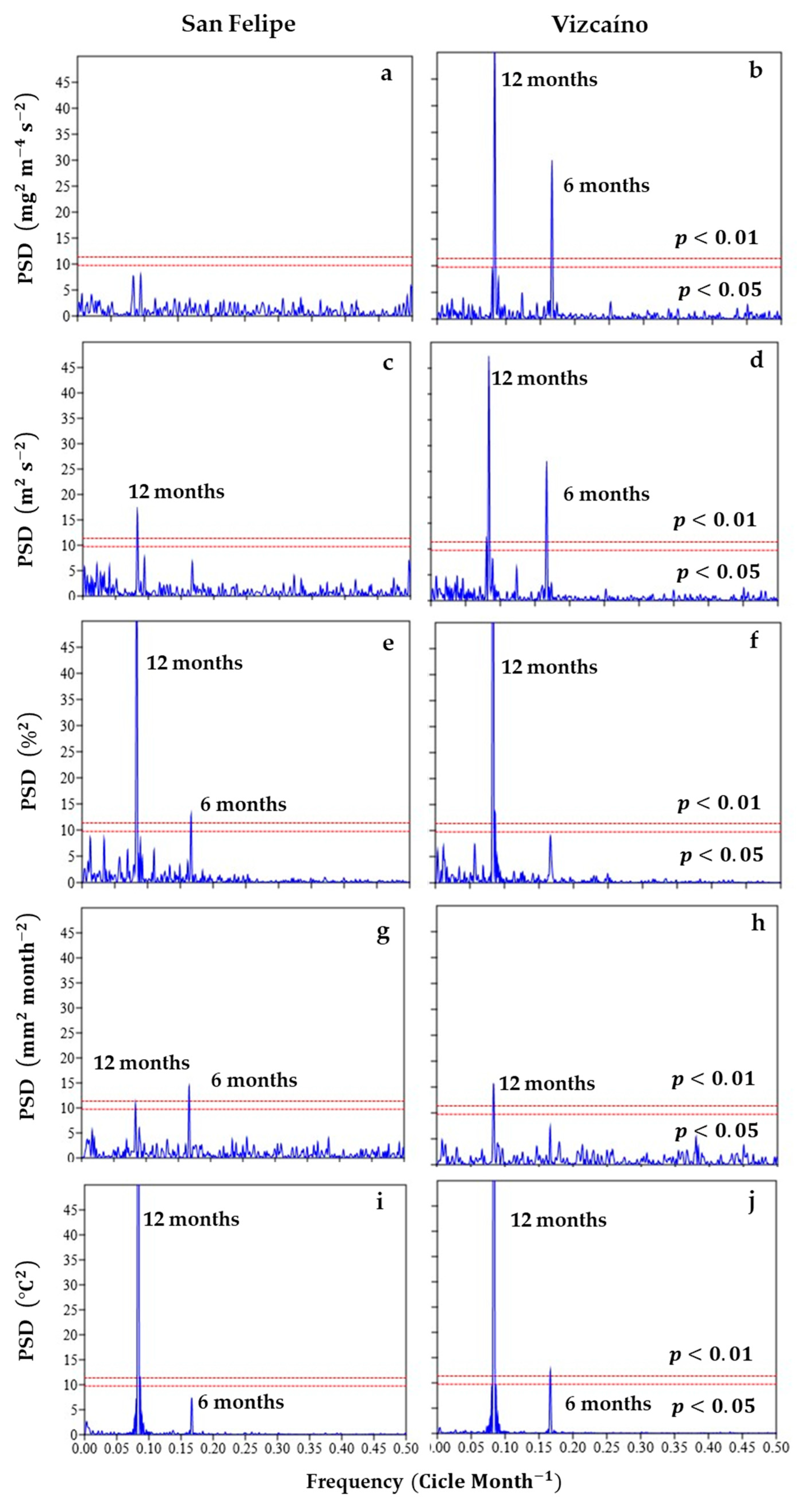
4.1. Intra-Annual Variability

The monthly climatologies of dust emission (Figure 2a) showed a unimodal behavior in San Felipe, with a peak in June (48.09 ${\mathrm{mg} \mathrm{m}}^{-2}{ \mathrm{d}}^{-1}$). Vizcaino showed a bimodal pattern, with peaks in April (353.35 ${\mathrm{mg} \mathrm{m}}^{-2}{ \mathrm{d}}^{-1}$) and October (150.15 ${\mathrm{mg} \mathrm{m}}^{-2}{ \mathrm{d}}^{-1}$). Wind speed (Figure 2b) displays a bimodal behavior with peaks in April (4.61 m s⁻¹) and October (3.60 m s⁻¹) for Vizcaíno, and a unimodal behavior with a peak in June (2.92 m s⁻¹) for San Felipe. The climatologies of the annual cycle of air temperature (Figure 2c) display a unimodal behavior in both regions, with a peak in August (28.6 °C in San Felipe and 26.50 °C in Vizcaíno). In addition, higher temperatures were recorded in San Felipe relative to Vizcaíno between April and October.

The climatologies of the annual cycle of soil moisture (Figure 2d) reveal the same variability in the two regions, with a minimum in June and a peak in January, the highest values predominated in Vizcaíno. Finally, precipitation (Figure 2e) showed a bimodal behavior in both regions, with peaks in August (1.75 mm month⁻¹) and February (1.66 mm month⁻¹) in San Felipe, and in December (2.11 mm month⁻¹) and September (1.64 mm month⁻¹) in Vizcaíno.

It is evident (Figure 2) that the peaks of dust emission flux are consistent with the peaks of wind speed and the minima of soil moisture and precipitation. The mean values for the variables in different seasons (Table 1) show peak dust emission flux in summer (17.41 ${\mathrm{mg} \mathrm{m}}^{-2}{ \mathrm{d}}^{-1}$) and spring (281.11 ${\mathrm{mg} \mathrm{m}}^{-2}{ \mathrm{d}}^{-1}$) for San Felipe and Vizcaino, respectively.

With regard to the meteorological variables (Table 1), optimal conditions for dust emission flux in San Felipe occurred during the summer, when low moisture (7.18%) and precipitation (0.7 mm month⁻¹) coincided with peak values of wind speed (2.62 m s⁻¹) and temperature (26.9 °C). In Vizcaino, minimum moisture (15.59%) coincided with maximum temperature (24.7 °C) in the summer, although the peak of wind speed (4.42 m s⁻¹) occurred in spring.

PSD showed two dominant peaks of energy at 12 and 6 months in dust emission flux and the hydrometeorological variables in the Vizcaino region (Figure 3b,d,f,h,j). San Felipe showed a single peak of energy at 12 months in wind speed, soil moisture, and precipitation (Figure 3c,e,g,i), and statistically significant peaks at six months in soil moisture and precipitation (Figure 3e,g). Dust emission flux showed a low annual signal below the established statistical significance.

A comparison between variance ellipses for wind in the different seasons of the year (Figure 4) shows the highest variability in winter in the two study regions (Figure 4). The standard deviation in the semi-axis of highest variability was 0.61 m s⁻¹ for San Felipe and 0.64 m s⁻¹ for Vizcaino (Table 2).

Average vectors for San Felipe showed a prevailing southeast direction pointing toward the GC, although the eastward direction dominated in summer. In Vizcaino, most vectors also pointed to the southeast, heading to the semi-axis of highest variability (Figure 4). Additionally, the major axis of the variability ellipses is perpendicular and parallel to the BCP in the San Felipe and Vizcaíno regions.

The lowest wind variability occurred during autumn and spring, with standard deviations on the semi-axis of highest variability of 0.38 m s⁻¹ and 0.45 m s⁻¹ for San Felipe and Vizcaino, respectively (Table 2).

During spring–summer, the axis of highest variability of wind speed showed similar behavior in Vizcaíno and San Felipe (~0.45 m s⁻¹). Mean wind speed was ~1.49 m s⁻¹ for Vizcaino (Table 2). Wind maps for the BCP region (Figure 4) show that the dominant wind direction is from the BCP to the GC, except during winter. The highest intensities predominated during spring and summer.

The association between Spearman’s correlation coefficients of Z-transformed variables vs. the significant components calculated in the PCA (

Table 3. Spearman’s correlation coefficients of the Z-transformed variables vs. the significant components calculated from the numeric version of the principal component analysis (PCA) for San Felipe and Vizcaino.

Z-Transformed Variables	San Felipe		Vizcaíno
	PC1	PC2	PC1	PC2
Z E	0.95	0.01	0.87	−0.39
Z v	0.80	0.03	0.91	−0.33
Z SVM	0.02	−0.75	−0.59	−0.73
Z T	0.01	0.96	0.12	0.88
Z Precp	0.02	−0.35	−0.65	−0.17

) revealed, through component 1 (which accounts for 37.15% and 46.25% of variance in San Felipe and Vizcaino, respectively), a direct association between dust emission flux and wind, except for the fact that dust emission flux and wind speed are inversely related to precipitation in Vizcaíno. In San Felipe component 2 (that explains 35.31% of variance), soil volumetric moisture and precipitation are directly related, with variables being controlled by temperature. Finally, in Vizcaino component 2 (31.55% of variance), moisture and temperature are inversely related (Table 3).

4.2. Interannual Variability, Trends in Dust Emissions Flux and Hydrometeorological Variables

Mean annual values of dust emission flux and hydrometeorological variables during the period 1979–2014 in San Felipe and Vizcaino deserts are shown in

Table 4. Mean annual dust emission flux and hydrometeorological variables during the period 1979–2014 for San Felipe (SF) and Vizcaino (VZ). N = 36.

Variable	Site	Mean
E (${\mathrm{mg} \mathrm{m}}^{-2}{ \mathrm{d}}^{-1}$)	SF	24.05
	Vz	170.77
v (${\mathrm{m} \mathrm{s}}^{-1}$)	SF	2.40
	Vz	3.66
T (°C)	SF	20.77
	Vz	20.05
SVM (%)	SF	10.10
	Vz	18.79
Precp (mm month−1)	SF	0.93
	Vz	1.01

. With regard to dust emission flux, values for Vizcaíno and San Felipe are 170.77 and 24.05 ${\mathrm{mg} \mathrm{m}}^{-2}{ \mathrm{d}}^{-1}$, respectively (Table 4).

The hydrometeorological variables reported higher values for wind speed (3.66 ${\mathrm{m} \mathrm{s}}^{-1}$), soil moisture (18.79%) and precipitation (1.01 mm month⁻¹) in Vizcaíno, while temperature (20.77 °C) was higher in San Felipe.

When the normality of the dataset is contrasted with the Shapiro and Wilk test [43], the null hypothesis is rejected for N = 36. Hence, the set of hydrometeorological data and dust emission flux is not normally distributed at a significance level of P < 0.05, as the statistics obtained are lower than the critical value provided by the tables (<0.935).

The trend analysis in the annual series (

Table 5. Modified non-parametric Mann–Kendall test (MKM): Positive trend (1) and negative trend (−1), (0) indicates that the null hypothesis is rejected at the significance level P < 0.05. The Theil-Sen (TS) estimator represents the slope for N = 36.

Site	Dust Emission Flux		Wind Speed		Temperature		Soil Volumetric Moisture		Precpitation
	MKM	TS	MKM	TS	MKM	TS	MKM	TS	MKM	TS
S. Felipe	1	0.31	1	0.01	1	0.03	−1	−0.01	−1	−0.01
Vizcaíno	1	0.85	1	0.01	1	0.01	−1	−0.03	−1	−0.01

) revealed that dust emission flux, wind speed, and temperature showed a positive trend, with increases of 0.31 ${\mathrm{mg} \mathrm{m}}^{-2}{ \mathrm{d}}^{-1}{\mathrm{yr}}^{-1}$, 0.01 ${\mathrm{m} \mathrm{s}}^{-1}{\mathrm{yr}}^{-1}$, and 0.03 °C ${\mathrm{yr}}^{-1}$ in San Felipe, and 0.85 ${\mathrm{mg} \mathrm{m}}^{-2}{ \mathrm{d}}^{-1}{\mathrm{yr}}^{-1}$, 0.01 ${\mathrm{m} \mathrm{s}}^{-1}{\mathrm{yr}}^{-1}$, and 0.01 °C ${\mathrm{yr}}^{-1}$ in Vizcaíno.

Precipitation (Table 5) showed a negative trend in both regions, with decreases of 0.01 mm ${\mathrm{y}}^{-1}$. For its part, soil moisture in Vizcaino showed a higher decrease rate (0.03% ${\mathrm{y}}^{-1}$) relative to San Felipe (0.01% ${\mathrm{y}}^{-1}$).

The associations between dust emission flux and hydrometeorological variables show that in San Felipe, dust emission flux is positively associated with air temperature $\left(\rho =0.74, P<0.05\right)$, while there is a negative association with soil volumetric moisture $\left(\rho =0.47, P<0.05\right)$ and precipitation $\left(\rho =-0.53, P<0.05\right)$ (

Table 6. Associations between annual dust emission flux (E) and hydrometeorological variables for N = 36 at a significance level of P < 0.05.

Site	T (°C)	SVM (%)	Precp (mm month−1)
E from San Felipe	0.74	−0.3	−0.72
E from Vizcaíno	0.51	−0.72	−0.41

).

In Vizcaino, Spearman’s correlation coefficient (Table 6) shows positive associations with air temperature $\left(\rho =0.51, P<0.05\right)$ and negative associations with precipitation $\left(\rho =-0.41, P<0.05\right)$and soil volumetric moisture $\left(\rho =-0.71, P<0.05\right)$.

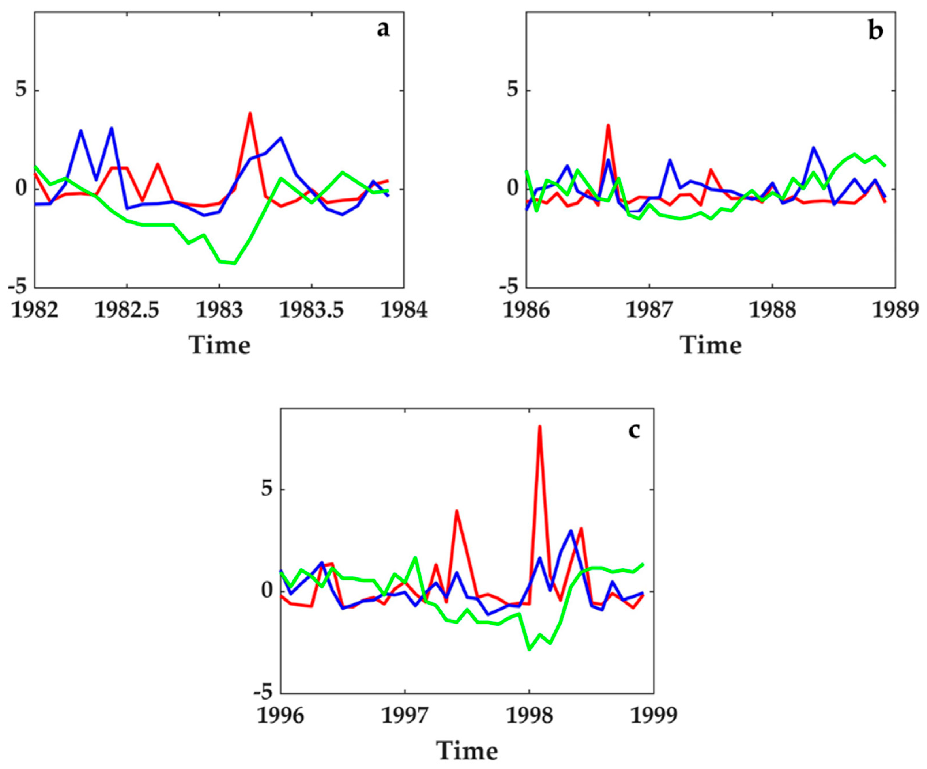
Influence of El Niño on Dust Emission Flux

The cross-correlation between the time series of El Niño and standardized anomalies of dust emission flux showed a lag of 19 months in San Felipe ($\rho =0.4, P<0.05$) and 21 months in Vizcaino ($\rho =0.33, P<0.05$), i.e., there are positive anomalies in dust emission flux after the onset of El Niño indicating a significant increase in dust production in both study areas.

The results obtained in the cross-correlation are shown in Figure 5. These show that when the climate event starts losing intensity, dust emission flux shows positive anomalies ranging between one and three standard deviations in both regions for each event studied.

5. Discussion

The differences between the location and geographical features of the study areas suggest, through the analysis of intra-annual variability, that dust emission flux rates are regulated by the synergy between hydrometeorological variables. Dust emissions flux are relevant when low soil moisture, high air temperature, and high wind speeds prevail.

Precipitation levels in the two desert areas during winter, spring, autumn, and summer, as calculated in the present study, are similar to those reported by Hastings and Turner [49].

Because of the extensive plains (elevation <200 m a.s.l.) between 26–28° N, Vizcaíno is affected by winds from the northwest (values in the Pacific off the BCP as reported by Castro and Martinez [50] and Morales-Acuña [26] are above $5 {\mathrm{m} \mathrm{s}}^{-1}$ in spring). In contrast, the natural barrier (elevation > 1200 m a.s.l.) located in the west margin of San Felipe (Figure 1) minimizes this effect.

The main feature found to affect the annual variability of the wind field in the region is the displacement during winter and summer (frequency ~6 months) of the North Pacific High-Pressure Center (NPHPC), located approximately at 32° N–140° W [51,52]. The findings using spectral analysis suggest that the influence of the NPHPC on dust emission flux and the hydrometeorological variables is intense not only in the Pacific Ocean decreasing toward the coast, as reported by Castro and Martinez [50], but also in Vizcaíno, being weaker in San Felipe, as reported by Salinas-Zavala et al. [24]. The above suggests that the climate conditions in Vizcaino are better suited for promoting dust events relative to San Felipe. Particularly, the seasonal variability of precipitation is attributed mainly to processes at local (upwelling) and global (El Niño) levels in addition to tropical cyclones and the passage of cold fronts [52,53].

The direction of average vectors of variance ellipses in the period of highest variability (winter) (Figure 4) indicates that the variability in wind speed partly responds to the winter pattern and the NPHPC, which in this season moves toward the equator (~25° N–125° W) producing strong pressure gradients and a component of wind blowing in the same direction of displacement (~40° N) [51].

The associations between dust emission flux and the hydrometeorological variables in each study area, using PCA analysis show that dust emission flux is driven mainly by fluctuations in wind speed, as reported by Pu and Ginoux [19] for deserts adjacent to our study area. These associations also highlight the direct relationship between soil moisture and precipitation, both controlled by temperature.

Annual averages of the hydrometeorological variables (Table 4) revealed that Vizcaíno showed higher values than San Felipe, due to its exposure to the northwest winds, the latitudinal and anomalous distribution of precipitation [53], and its proximity to the California Current [52]. Separately, dust emission flux rates are higher in Vizcaíno than in San Felipe. Annual precipitation values are consistent with those reported by Arriaga-Ramírez and Cavazos [53] for the middle of the Baja California Peninsula, north of Sonora, and southwest Arizona.

A comparison between annual emissions in San Felipe and MD fluxes reported by Muñoz-Barbosa et al. [20] and Félix-Bermúdez et al. [54] for the regions of San Felipe and Ensenada Bay (a region adjacent to the San Felipe desert), respectively (

Table 7. Dust emission flux $\left({\mathrm{E}, \mathrm{mg} \mathrm{m}}^{-2}{\mathrm{d}}^{-1}\right)$ for different desert regions of the world.

	E	Desert	Reference
Winter	71.98	Vizcaíno	This Study
	15.92	San Felipe
Spring	277.52	Vizcaíno
	15.58	San Felipe
Autumn	102.77	Vizcaíno
	12.44	San Felipe
Summer	113.81	Vizcaíno
	16.87	San Felipe
Average	170.77	Vizcaíno
	24.05	San Felipe
Annual Average	23	San Felipe, México	[20]
	22	Puerto Peñasco, México
	23.33	Todos Santos Bay, México	[54]
	399.04–467.54	Sahara, Africa	[55]
	206.6–341	Sahel, Africa
Dust Storm	2332	Taklimakan, China	[56]
	2592	Gobi, China
Dust Storm	1900	Eastern Mojave, US	[57]
Annual Average	174.21–226.02	Sahara, Africa	[56]
Dust Storm	864	Simpson, Australia	[12]
Seasonal	6.13 a, 31b, 12.05 c and 2.96 d	Gobi, China	[58]

Dust emission for: ^a winter, ^b spring, ^c autumn, and ^d summer.

) identified a rising trend, thereby reflecting increases in dust emission flux that is consistent with those obtained by Pu and Ginoux [19] for the BCP. The collate of MD emissions in the most relevant desert areas worldwide (Table 7) with atmospheric inputs of MD from the Vizcaíno and San Felipe deserts evidence that Vizcaíno is an important source of dust emission flux, since its mean annual emission (170.77 ${\mathrm{mg} \mathrm{m}}^{-2}{ \mathrm{d}}^{-1}$) is of the same order of magnitude as emissions from the Sahel and Sahara deserts [55,56].

The comparison of seasonal dust emission flux recorded in Vizcaíno and San Felipe (Table 7) with the standardized emissions per unit area reported by Xuan et al. [58] for northern China (Gobi desert) show that peak dust emission flux occurs in spring, as observed in Vizcaíno. Besides, MD emissions per unit area in Vizcaíno and San Felipe are higher than those in the Gobi desert (Table 7).

The trend analysis of the hydrometeorological variables (Table 5) identified increasing trends in wind speed and temperature. The rising trend in temperature observed in this study is consistent with the one reported by Blunden et al. [59], who reported positive anomalies of air temperature ranging between 1 °C and 5 °C in Vizcaino and San Felipe for the period 1981–2010. In addition, our positive trends confirm the reports of Englehart and Douglas [60] and Pavia et al. [61] regarding a shift to positive trends in the period between 1970 and 2004 in Mexico. Our results are also consistent with those reported by Prein et al. [62] for the southwest United States. The decrease in precipitation observed in this work is consistent with the one reported by Blunden et al. [59] for northern Baja California and differs from the results obtained by Arriaga-Ramírez and Cavazos [53] for the central part of the BCP, northern Sonora, and southwest Arizona, where annual series show no statistically significant trend. The negative trends for soil moisture coincide with a lower amount of humidity caused by the decrease in precipitation and the rising of air temperature.

Regarding trends in dust emission flux, the increases found for the past four decades are consistent with the rise in dust emission flux from spring to autumn reported by Pu and Ginoux [19]. The association between dust emission flux and hydrometeorological variables (Table 6) is consistent with studies conducted in southeastern United States [19], China, and Mongolia [18], suggesting that increases in dust emission flux in recent decades are regulated by variations in wind speed, temperature, precipitation, and the extension of bare soil. The lag in the occurrence of relevant dust emission flux due to El Niño events (strong and very strong) observed in this work is consistent with Okin and Reheis [16] in the southwestern United States. In our study area, such effects can be explained by the impact of this climate phenomenon on precipitation in the BCP [52,63,64].

Regarding the potential implications of the dust deposition in surface waters of adjacent seas, if the particles contains Fe, Cu, or Cd, these metals may affect primary production [65,66,67], as they play a key role in biogeochemical processes such as photosynthesis [68]. Studies on dissolved Fe suggest that it may be a limiting element for primary production [20]. Félix-Bermúdez et al. [54] suggest that the impact of dissolved Fe on marine ecosystems probably depends on the composition of water in terms of the N:Fe ratio. Accordingly, when water is already enriched with Fe, the atmospheric iron deposited will be an additional source of a non-limiting nutrient and N will probably act as the limiting element for primary production. Otherwise, dissolved Fe will be the limiting nutrient with a key role as a driver of primary production.

6. Conclusions

This study showed that seasonal and inter-annual variability in dust emission flux in the Vizcaíno and San Felipe desert areas is controlled by fluctuations in the hydrometeorological variables and that these, in turn, may respond to the influence of the NPHPC. Consequently, under optimal hydrometeorological conditions, dust emission flux peaks in summer (San Felipe) and spring (Vizcaíno).

The increases in dust emission flux during the study period (1979–2014) are associated with the rising trends in wind speed and air temperature, and with the decreases in moisture and precipitation that varied in both desert regions.

In addition, the frequency and intensity of dust events in San Felipe and Vizcaino appear to be related to strong and very strong ENSO events, with lags of 19 and 21 months in San Felipe and Vizcaino, respectively.

Finally, given the amount of dust emitted from each desert areas evaluated and the rising trend in these emissions, the BCP should be considered as a significant source of dust at local and regional levels.

References

1. Shao, Y.; Wyrwoll, K.H.; Chappell, A.; Huang, J.; Lin, Z.; McTainsh, G.H.; Mikami, M.; Tanaka, T.Y.; Wang, X.; Yoon, S. Dust cycle: An emerging core theme in Earth system science. Aeolian Res. 2011, 2, 181–204. [Google Scholar] [CrossRef]
2. Haustein, K.; Washington, R.; King, J.; Wiggs, G.; Thomas, D.S.G.; Eckardt, F.D.; Bryant, R.G.; Menut, L. Testing the performance of state-of-the-art dust emission schemes using DO4Models field data. Geosci. Model Dev. 2015, 8, 341–362. [Google Scholar] [CrossRef] [Green Version]
3. Shao, Y. Physics and Modelling of Wind Erosion; Springer Science & Business Media: Berlin, Germany, 2008; Volume 37. [Google Scholar]
4. Shao, Y.P.; Raupach, M.R.; Leys, J.F. Leys A model for predicting aeolian sand drift and dust entrainment on scales from paddock to region. Soil Res. 1996, 34, 309–342. [Google Scholar] [CrossRef]
5. Westphal, D.L.; Toon, O.B.; Carlson, T.N. A two-dimensional numerical investigation of the dynamics and microphysics of Saharan dust storms. J. Geophys. Res. Atmos. 1987, 92, 3027–3049. [Google Scholar] [CrossRef]
6. Westphal, D.L.; Toon, O.B.; Carlson, T.N. A Case Study of Mobilization and Transport of Saharan Dust. J. Atmos. Sci. 1988, 45, 2145–2175. [Google Scholar] [CrossRef] [Green Version]
7. Nickling, W.G.; Gillies, J.A. Dust emission and transport in Mali, West Africa. Sedimentology 1993, 40, 859–868. [Google Scholar] [CrossRef]
8. Ginoux, P.; Prospero, J.M.; Gill, T.E.; Hsu, N.C.; Zhao, M. Global-scale attribution of anthropogenic and natural dust sources and their emission rates based on MODIS Deep Blue aerosol products. Rev. Geophys. 2012, 50. [Google Scholar] [CrossRef]
9. Gillette, D.A. Fine Particulate Emissions Due to Wind Erosion. Trans. ASAE 1977, 20, 890–897. [Google Scholar] [CrossRef]
10. Gillette, D.A.; Passi, R. Modeling dust emission caused by wind erosion. J. Geophys. Res. Atmos. 1988, 93, 14233–14242. [Google Scholar] [CrossRef] [Green Version]
11. Marticorena, B.; Bergametti, G. Modeling the Atmospheric Dust Cycle: 1. Design of a Soil-Derived Dust Emission Scheme. Available online: https://agupubs.onlinelibrary.wiley.com/doi/10.1029/95JD00690. (accessed on 10 September 2019).
12. Lu, H.; Shao, Y. Toward quantitative prediction of dust storms: an integrated wind erosion modelling system and its applications. Environ. Model. Softw. 2001, 16, 233–249. [Google Scholar] [CrossRef]
13. Ginoux, P.; Chin, M.; Tegen, I.; Prospero, J.M.; Holben, B.; Dubovik, O.; Lin, S.J. Sources and distributions of dust aerosols simulated with the GOCART model. J. Geophys. Res. Atmos. 2001, 106, 20255–20273. [Google Scholar] [CrossRef]
14. Nickovic, S.; Kallos, G.; Papadopoulos, A.; Kakaliagou, O. A model for prediction of desert dust cycle in the atmosphere. J. Geophys. Res. Atmos. 2001, 106, 18113–18129. [Google Scholar] [CrossRef] [Green Version]
15. Shao, Y. Simplification of a dust emission scheme and comparison with data. J. Geophys. Res. Atmos. 2004, 109. [Google Scholar] [CrossRef] [Green Version]
16. Okin, G.S.; Reheis, M.C. An ENSO predictor of dust emission in the southwestern United States. Geophys. Res. Lett. 2002, 29. [Google Scholar] [CrossRef]
17. Ji, Z.; Wang, G.; Pal, J.S.; Yu, M. Potential climate effect of mineral aerosols over West Africa: Part II—Contribution of dust and land cover to future climate change. Clim. Dyn. 2018, 50, 2335–2353. [Google Scholar] [CrossRef]
18. Song, H.; Wang, K.; Zhang, Y.; Hong, C.; Zhou, Y.S. Simulation and evaluation of dust emissions with WRF-Chem (v3.7.1) and its relationship to the changing climate over East Asia from 1980 to 2015. Atmos. Environ. 2017, 167, 511–522. [Google Scholar] [CrossRef]
19. Pu, B.; Ginoux, P. Projection of American dustiness in the late 21st century due to climate change. Sci. Rep. 2017, 7, 1–10. [Google Scholar] [CrossRef] [Green Version]
20. Muñoz-Barbosa, A.; Segovia-Zavala, J.A.; Huerta-Diaz, M.A. Atmospheric iron fluxes in the northern region of the Gulf of California: Implications for primary production and potential. Deep Sea Res. Part Oceanogr. Res. Pap. 2017, 129, 69–79. [Google Scholar] [CrossRef]
21. Morales-Acuña, E.; Torres, C.R.; Linero-Cueto, J.R. Surface wind characteristics over Baja California Peninsula during summer. Reg. Stud. Mar. Sci. 2019, 29, 100654. [Google Scholar] [CrossRef]
22. SEMARNAT. Informe de la Situación del Medio Ambiente en México. Compendio de Estadísticas Ambientales. Indicadores Clave, de Desempeño Ambiental y de Crecimiento Verde; Semarnat: Mexico City, Mexico, 2016.
23. Ivanova, A.; Gámez, A. Baja California Sur Ante el Cambio Climático: Vulnerabilidad, Mitigación y Adaptación. Estudios Para la Elaboración Del Plan Estatal de Acción Ante el Cambio Climático (PEACC-BCS); UABCS, CIBNOR, CICIMAR, CICESE, CONACYT, INE, SEMARNAT, La Paz, BCS, Eds.; Diario Oficial de la Federación: Mexico City, Mexico, 2012; ISBN 978-607-7777-31-1.
24. Salinas-Zavala, C.A.; Martínez-Rincón, R.O.; Morales-Zárate, M.V. Tendencia en el siglo XXI del Índice de Diferencias Normalizadas de Vegetación (NDVI) en la parte sur de la península de Baja California. Investigaciones Geográficas 2017, 94, 82–90. [Google Scholar] [CrossRef]
25. González-Abraham, C.E.; Garcillán, P.P.; Ezcurra, E. Grupo de trabajo de ecorregiones Ecorregiones de la península de Baja California: Una síntesis. Bol. Soc. Botánica México 2010, 87, 69–82. [Google Scholar]
26. Morales-Acuña, E. Influencia de la Viriabilidad Espacio-Temporal del Viento en el Transporte de Polvo Hacia el Golfo de California. Ph.D. Thesis, Instituto Politécnico Nacional. Centro Interdisciplinario de Ciencias Marinas, La Paz, Bolivia, 2015. [Google Scholar]
27. INEGI. Síntesis de Información Geográfica del Estado de Baja California; Instituto Nacional de Estadística, Geografía e Informática: Mexico City, Mexico, 2010. [Google Scholar]
28. Turrent, C.; Zaitsev, O. Seasonal Cycle of the Near-Surface Diurnal Wind Field Over the Bay of La Paz, Mexico. Bound. Layer Meteorol. 2014, 151, 353–371. [Google Scholar] [CrossRef]
29. Dominguez-Pérez, D.-A. Influencia de los Sistemas de Brisas Marinas en el Desarrollo de Precipitación Sobre la Península de Baja California; Centro de Investigación Científica y de Educación Superior de Ensenada: Ensenada, Mexico, 2017. [Google Scholar]
30. Carlos, T.N.; Sergio, L.C.; Adán, M.T.; Jaime, G.T.; Mariana, M.C.; Eduardo, G.S. Numerical experiments of wind circulation off Baja California coast. In Experimental and Computational Fluid Mechanics; Klapp, J., Medina, A., Eds.; Springer International Publishing: Cham, Switzerland, 2014; pp. 327–339. [Google Scholar]
31. Torres, C.R.; Lanz, E.E.; Larios, S.I. Effect of wind direction and orography on flow structures at Baja California Coast: A numerical approach. J. Comput. Appl. Math. 2016, 295, 48–61. [Google Scholar] [CrossRef]
32. Torres-Navarrete, C.R.; Larios, S.I. Modelling Three-Dimensional Winds on a NW Pacific Region of Mexico Using Boundary-Fitted Grids. Open J. Mar. Sci. 2016, 7, 327–339. [Google Scholar] [CrossRef]
33. Shao, Y.; Raupach, M.; Fimdlater, P. Effect of Saltation Bombardment on the Entrainment of Dust by Wind. J. Geophys. Res. Atmos. 1993, 98, 12719–12726. [Google Scholar] [CrossRef]
34. Tegen, I.; Fung, I. Modeling of mineral dust in the atmosphere: Sources, transport, and optical thickness. J. Geophys. Res. Atmos. 1994, 99, 22897–22914. [Google Scholar] [CrossRef]
35. Monin, A.S.; Yaglom, A.M. Statistical Fluid Mechanics—Vol 1: Mechanics of Turbulence, 1st ed.; MIT Press: Cambridge, MA, USA, 1971. [Google Scholar]
36. Lonin, S.A.; Linero, J. Parametrización de rugosidad de la superficie del mar bajo la inestabilidad de la capa próxima y la edad del oleaje. Boletín Científico 2009, 27, 22–28. [Google Scholar] [CrossRef]
37. Wieringa, J. Updating the Davenport roughness classification. J. Wind Eng. Ind. Aerodyn. 1992, 41, 357–368. [Google Scholar] [CrossRef]
38. Song, X.; Zhang, H.; Chen, J.; Park, S. Flux–Gradient Relationships in the Atmospheric Surface Layer Over the Gobi Desert in China. Bound. Layer Meteorol. 2010, 134, 487–498. [Google Scholar] [CrossRef]
39. Pasquill, F. The Estimation of the Dispersion of Windborne Material. Meteorol. Mag. 1961, 90, 33–49. [Google Scholar]
40. Stull, R.B. An Introduction to Boundary Layer Meteorology; Springer: Amsterdam, The Netherlands, 1988. [Google Scholar]
41. Thomson, R.E.; Emery, W.J. Data Analysis Methods in Physical Oceanography; Newnes: Oxford, UK, 2014. [Google Scholar]
42. Santamaría-del-Ángel, E.; González-Silvera, A.; Millán-Núñez, R.; Cajal-Medrano, R. Determining dynamic biogeographic regions using remote sensing data. In Handbook of Satellite Remote Sensing Image Interpretation: Applications for Marine Living Resources Conservation and Management; U PRESPO and IOCCG: Dartmouth, NS, Canada, 2011; pp. 273–293. [Google Scholar]
43. Shapiro, S.S.; Wilk, M.B. An Analysis of Variance Test for Normality (Complete Samples). Biometrika 1965, 52, 591–611. [Google Scholar] [CrossRef]
44. Hamed, K.H.; Rao, A.R. A modified Mann-Kendall trend test for autocorrelated data. J. Hydrol. 1998, 204, 182–196. [Google Scholar] [CrossRef]
45. Dahmen, E.R.; Hall, M.J. Screening of Hydrological Data: Tests for Stationarity and Relative Consistency; ILRI: Wageningen, The Netherlands, 1990. [Google Scholar]
46. Sen, P.K. Estimates of the Regression Coefficient Based on Kendall’s Tau. J. Am. Stat. Assoc. 1968, 63, 1379–1389. [Google Scholar] [CrossRef]
47. Santamaría-del-Angel, E.; Millán-Núñez, R.; Cajal-Medrano, R. Effect of Turbulent Kinetic Energy on The Spatial Distribution of Chlorophyll a in a Small Coastal Lagoon. Ciencias Marinas 1992, 18, 1–16. [Google Scholar] [CrossRef]
48. Azaria, M.; Hertz, D. Time delay estimation by generalized cross correlation methods. IEEE Trans. Acoust. Speech Signal Process. 1984, 32, 280–285. [Google Scholar] [CrossRef]
49. Hastings, J.R.; Turner, R.M. Seasonal Precipitation Regimes in Baja California, Mexico. Geogr. Ann. Ser. Phys. Geogr. 1965, 47, 204–223. [Google Scholar] [CrossRef]
50. Castro, R.; Martínez, J. Variabilidad espacial y temporal del campo de viento. In Dinámica Del Ecosistema Pelágico Frente a Baja California; Instituto Nacional de Ecología: Coyoacán, Mexico, 2010; p. 19. [Google Scholar]
51. Romero-Centeno, R.; Zavala-Hidalgo, J.; Raga, G.B. Midsummer Gap Winds and Low-Level Circulation over the Eastern Tropical Pacific. J. Clim. 2007, 20, 3768–3784. [Google Scholar] [CrossRef] [Green Version]
52. Minnich, R.A.; Vizcaino, E.F.; Dezzani, R.J. The El Niño/Southern Oscillation and Precipitation Variability in Baja California, Mexico. Atmósfera 2009, 13, 1–20. [Google Scholar]
53. Arriaga-Ramírez, S.; Cavazos, T. Regional trends of daily precipitation indices in northwest Mexico and southwest United States. J. Geophys. Res. Atmos. 2010, 115. [Google Scholar] [CrossRef]
54. Félix-Bermúdez, A.; Delgadillo-Hinojosa, F.; Huerta-Diaz, M.A.; Camacho-Ibar, V.; Torres-Delgado, E.V. Atmospheric Inputs of Iron and Manganese to Coastal Waters of the Southern California Current System: Seasonality, Santa Ana Winds, and Biogeochemical Implications. J. Geophys. Res. Oceans 2017, 122, 9230–9254. [Google Scholar] [CrossRef]
55. Kim, K.H.; Choi, G.H.; Kang, C.H.; Lee, J.H.; Kim, J.Y.; Youn, Y.H.; Lee, S.R. The chemical composition of fine and coarse particles in relation with the Asian Dust events. Atmos. Environ. 2003, 37, 753–765. [Google Scholar] [CrossRef]
56. Laurent, B.; Marticorena, B.; Bergametti, G.; Léon, J.F.; Mahowald, N.M. Modeling mineral dust emissions from the Sahara desert using new surface properties and soil database. J. Geophys. Res. Atmos. 2008, 113. [Google Scholar] [CrossRef] [Green Version]
57. Sweeney, M.R.; McDonald, E.V.; Etyemezian, V. Quantifying dust emissions from desert landforms, eastern Mojave Desert, USA. Geomorphology 2011, 135, 21–34. [Google Scholar] [CrossRef]
58. Xuan, J.; Liu, G.; Du, K. Dust emission inventory in Northern China. Atmos. Environ. 2000, 34, 4565–4570. [Google Scholar] [CrossRef]
59. Blunden, J.; Arndt, D.S. State of the Climate in 2015. Bull. Am. Meteorol. Soc. 2016, 97, S1–S275. [Google Scholar] [CrossRef]
60. Englehart, P.J.; Douglas, A.V. Changing behavior in the diurnal range of surface air temperatures over Mexico. Geophys. Res. Lett. 2005, 32. [Google Scholar] [CrossRef]
61. Pavia, G.; Graef, F.; Reyes, J. Annual and seasonal surface air temperature trends in Mexico. Int. J. Climatol. 2009, 29, 1324–1329. [Google Scholar] [CrossRef]
62. Prein, A.F.; Holland, G.J.; Rasmussen, R.M.; Clark, M.P.; Tye, M.R. Running dry: The US Southwest’s drift into a drier climate state. Geophys. Res. Lett. 2016, 43, 1272–1279. [Google Scholar] [CrossRef]
63. Rodríguez-Moreno, V.M.; Bullock, S.H. Vegetation response to rainfall pulses in the Sonoran Desert as modelled through remotely sensed imageries. Int. J. Climatol. 2014, 34, 3967–3976. [Google Scholar] [CrossRef]
64. Magaña, V.; Pérez, J.; Conde, C. El fenómeno del el niño y la oscilación del sur. Sus impactos en México—Revista Ciencias. Revista Ciencias UNAM 1998, 51, 14–18. [Google Scholar]
65. Segovia-Zavala, J.A.; Delgadillo-Hinojosa, F.; Lares-Reyes, M.L.; Huerta-Díaz, M.A.; Muñoz-Barbosa, A.; Torres-Delgado, E.V. Atmospheric input and concentration of dissolved iron in the surface layer of the Gulf of California. Ciencias Marinas 2009, 35, 75–90. [Google Scholar] [CrossRef]
66. Segovia-Zavala, J.A.; Lares, M.L.; Delgadillo-Hinojosa, F.; Tovar-Sánchez, A.; Sañudo-Wilhelmy, S.A. Dissolved iron distributions in the central region of the Gulf of California, México. Deep Sea Res. Part Oceanogr. Res. Pap. 2010, 57, 53–64. [Google Scholar] [CrossRef]
67. Segovia-Zavala, J.A.; Delgadillo-Hinojosa, F.; Lares-Reyes, M.L.; Huerta-Díaz, M.A.; Muñoz-Barbosa, A.; del Angel, E.S.M.; Torres-Delgado, E.V.; Sañudo-Wilhelmy, S.A. Vertical distribution of dissolved iron, copper, and cadmium in Ballenas Channel, Gulf of California. Ciencias Marinas 2011, 37, 457–469. [Google Scholar] [CrossRef] [Green Version]
68. Jickells, T.D.; An, Z.S.; Andersen, K.K.; Baker, A.R.; Bergametti, G.; Brooks, N.; Cao, J.J.; Boyd, P.W.; Duce, R.A.; Hunter, K.A.; et al. Global Iron Connections Between Desert Dust, Ocean Biogeochemistry, and Climate. Science 2005, 308, 67–71. [Google Scholar] [CrossRef] [Green Version]
Figure 1. Map of the study area showing the location of the sources of dust at San Felipe and Vizcaino (black dots). It also shows the orography of the BCP from Etopo 1 global data with a 1 arcmin resolution.
Atmosphere 10 00582 g001
Figure 2. Monthly climatologies for (a) dust emission flux (E), (b) wind speed (v), (c) air temperature (T), (d) soil volumetric moisture (SVM), and (e) precipitation (Precp). Vizcaino (blue line) and San Felipe (red line) for the period from January 1979 to December 2014.
Atmosphere 10 00582 g002
Figure 3. Power spectral density (PSD) for monthly averages of time series: Dust emission flux (a,b), wind speed (c,d), soil volumetric moisture (e,f), precipitation (g,h), and air temperature (i,j) from January 1979 to December 2014.
Atmosphere 10 00582 g003
Figure 4. Average vectors for wind speed and variance ellipses (red line) for Vizcaíno and San Felipe, for the period from January 1979 to December 2014 for the BCP. Colorbar denotes wind speed.
Atmosphere 10 00582 g004
Figure 5. Standardized anomalies of dust emission flux in San Felipe (red) and Vizcaino (blue) on the SOI (green). El Niño 1982–1983 (a), 1987–1988 (b), and 1997–1998 (c).
Atmosphere 10 00582 g005