
Cancer Classification Utilizing Voting Classifier with Ensemble Feature Selection Method and Transcriptomic Data

 , ,
, ,  ,
,  , , and
Abstract
:1. Introduction
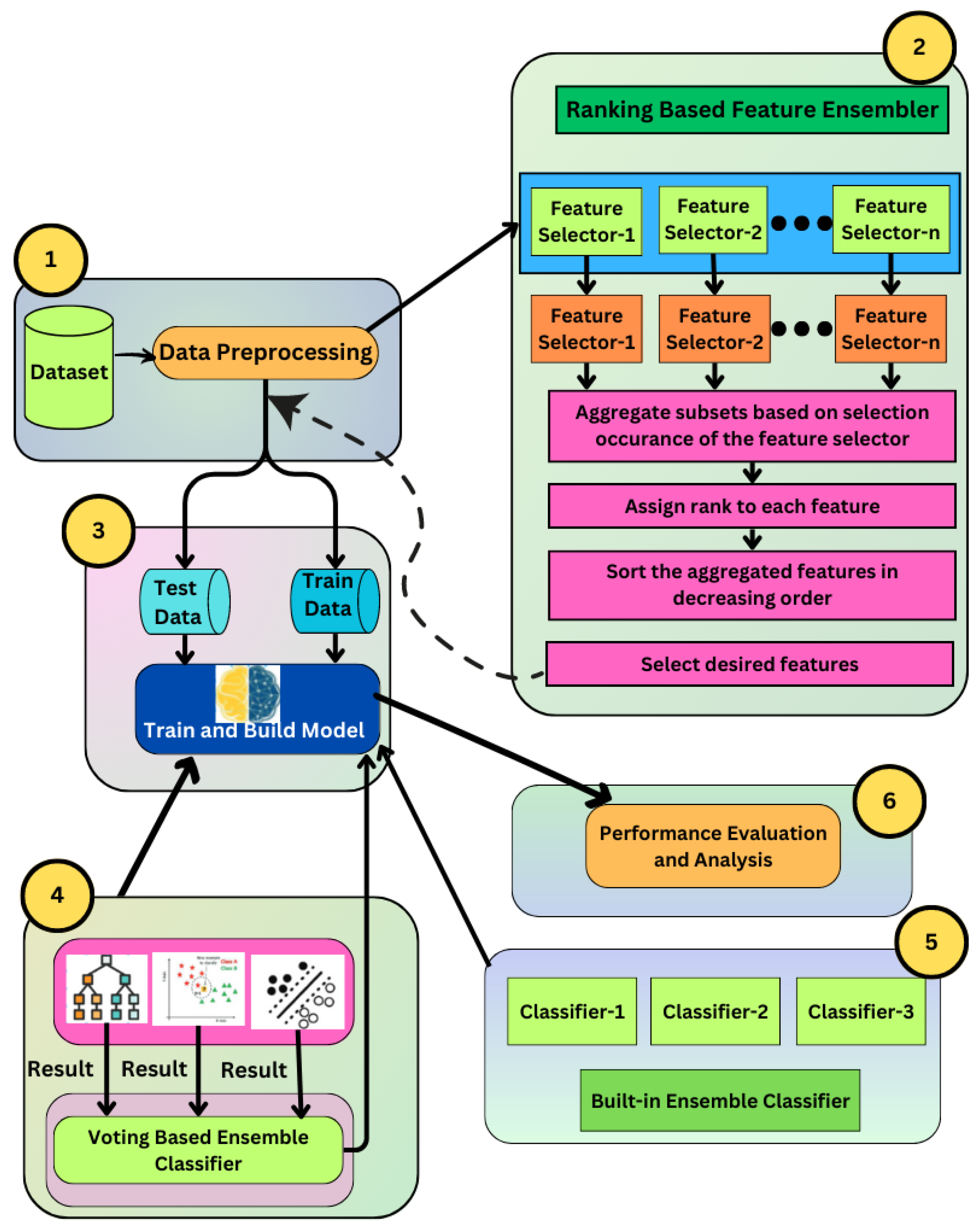
- We proposed an effective rank-based ensemble feature selection approach as well as an ensemble voting classifier model that can perform cancer classification with substantially high accuracy.
- The rank-based ensemble feature selection approach selects the most influential and relevant features that improve the cancer detection performance by utilizing several feature selection techniques, namely PCA, recursive feature elimination, Pearson correlation, ridge regression, and variance threshold.
- The ensemble classifier model was developed using an average weighted voting classifier on several ML algorithms, including SVM, KNN, and DT, to enhance the effectiveness of our model.
- Finally, the model was evaluated with three prominent cancer datasets. The performance results show that our proposed method outperforms the existing works with the selected features.
2. Preliminaries
Related Works
3. Methodology
- For the preprocessing of three experimental cancer datasets that were used in this study, namely leukemia, colon, and the 11-tumor dataset, unnecessary columns, missing values, and duplicate rows were removed, followed by label encoding and normalization.
- Next, significant and relevant features were extracted from the preprocessed data using different feature selection methods (FSMs), such as PCA, recursive feature elimination, Pearson correlation, ridge regression, and variance threshold, as well as our suggested rank-based ensemble feature selection method, by integrating multiple feature selection approaches.
- Then, the data split was conducted with a 70:30 ratio between the train and test datasets, with the training dataset serving as a calibration dataset for the model’s parameters and the test dataset serving as an evaluation dataset for performance.
- Then, the reduced dataset was evaluated using appropriate classification assessment metrics for a variety of ML classifiers, including KNN, DT, SVM, and proposed voting classifiers.
- We further compared the proposed voting classifier with the built-in ensemble classifiers such as AdaBoost (AB), gradient boost (GB), and random forest (RF).
3.1. Data Acquisition and Preprocessing
3.2. Proposed Rank-Based Ensemble Feature Selection Approach
- Ensemble-1 (E1): Select aggregated features with a frequency of occurrence greater than one. That is the feature selected by at least two FS methods.
- Ensemble-2 (E2): Select aggregated features with a frequency of occurrence greater than two. Thus, the feature is selected by at least three FS methods.
- Ensemble-3 (E3): In the third approach, features selected by more than three FS methods are chosen.
| Algorithm 1 Rank-based ensemble feature selection |
Initialize each sub-feature set: .
|
3.3. Proposed Ensemble Voting Classifier for Cancer Detection
| Algorithm 2 Majority voting ensemble classifier |
|
Input: - L: Labeled tuples for training of each class C with selected features. - D: Set of tuples for evaluation. - T: Set of tuples for testing. - N: (, , , …, ) Set of classifier ML algorithm.
|
3.4. Adopted Feature Selection Methods
- Principal Component Analysis: In nature, cancer data sets have substantially large dimensions. Hence, the number of features is reduced using the principal component analysis (PCA) technique. PCA is an orthogonal linear transformation that converts data to a new dimension system with the biggest variance of any projection of the data falling on the first dimension (called the first principal component), the second-best variance on the second dimension, etc. This method converts a set of observations of possibly correlated variables into a set of uncorrelated variables known as principal components via an orthogonal transformation [54]. The dimensions of various data sets are reduced using this strategy.
- Recursive Feature Elimination (RFE): RFE is a popular method as it is simple to implement and use and is effective in determining which features (columns) in a train set are more or less helpful in determining the target variable. RFE assesses the features by significance and returns the top-n features after removing the least important ones, where n is the users’ input. To use it, the class with the argument is first set up by specifying the algorithm to use and the argument by specifying the number of features to select. To pick the features, the class has to be suited to a training dataset using the function after it has been configured. In our study, we used the SVM algorithm as an as well as setting to 5490 for the leukemia dataset, 1000 for the colon dataset, and 5500 for the 11-tumor dataset.
- Pearson Correlation Coefficient: Pearson correlation and Spearman correlation are both measures of association or correlation between two variables, but they serve different purposes and have different strengths and weaknesses. The Pearson correlation coefficient is preferred when the underlying assumption of the relationship is considered to be linear. However, for the Spearman correlation, this assumption is not mandatory, i.e., the variables could be non-linearly related. As we were interested in finding a linear relationship, we used the former one, i.e., the Pearson correlation. Moreover, the types of data that we were dealing with were continuous, which also suits the Pearson correlation metric, whereas the Spearman correlation metric is suitable for ordinal, interval, or ratio data, which was not the case for us in this study. Pearson correlation shows how closely two variables are related linearly. Features with a strong association are more linearly dependent and hence affect the dependent variable in a similar way. If there is a strong association between two traits, one of them might be removed. Only metric variables are appropriate for PC. A correlation coefficient r is a number that ranges from −1 to +1: near 0 means a low association (an exact 0 implies no correlation); closer to 1 indicates a strong positive relationship; and near −1 indicates a strong negative relationship. For feature X having values x and classes C having values c, where X and C are viewed as random variables, Pearson’s linear correlation coefficient is calculated as [55]:In our study, we compared feature correlations and eliminated one of two features with a correlation greater than 0.9 (leukemia and colon dataset) and 0.6 (11-tumor dataset).
- Ridge Regression: Ridge regression is a prominent method for predicting data that makes use of regularization. Overfitting is a problem that regularization aims to solve. When there is a huge data collection with thousands of features and entries, overfitting becomes an apparent problem. When the data contain features that are certain to be more relevant and valuable, RR performs better. When a large number of characteristics are included, it is commonly employed to create parsimonious models. It applies L2 regularization, which entails adding a penalty equal to the square of the coefficients’ magnitude. Thus, RR optimizes the following:Here, RSS refers to the “Residual Sum of Squares”, which is nothing but the total of the square of mistakes between the predicted and actual values in the training data set, and alpha is the parameter that balances the degree of significance given to lessening RSS vs. minimizing the total of the square of coefficients, where alpha can take various values. In our study, we used alpha values of 0.3 (leukemia and 11-tumor datasets) and 0.4 (colon dataset).
- Variance Threshold: A simple baseline technique for selecting features is the variance threshold. It eliminates all features whose variance falls below a threshold value. All zero-variance characteristics are removed by default; that is, characteristics that have the same value across all samples. We feel that characteristics with a greater variance include more important data. To apply the variance threshold feature selection method, a variance threshold value (i.e., 0.1, 0.2 etc.) is chosen. The minimum variance that a feature must have to qualify as informative is determined by this threshold. Choosing the appropriate threshold value is crucial; a higher threshold retains only features with higher variance, while a lower threshold retains more features. The choice should align with the nature of the dataset. In our work, we have used different threshold values for different datasets.
3.5. Adopted ML Algorithm for Voting Classifier
- K-Nearest neighbors: For handling classification problems, the k-nearest neighbors (KNNs) technique is a simple supervised ML algorithm. The KNN algorithm believes that similar objects are close together. The KNN algorithm compares the k closest data points in the training data set based on resemblance metrics to determine the label of input data for a given new data [56]. In this system, the conclusion is selected by a majority vote of its neighbors. Because it requires zero experience and builds a fresh model for every experiment, this algorithm is one of the most efficient ML algorithms available. If the number of instances in the input data set grows, testing may become expensive. In our research, we only use one parameter in the model creation. is set to 3, which means 3 neighborhood points are required for classifying a given point.
- Support Vector Machine: The support vector machine (SVM) was first presented by [57]. SVM is a supervised learning algorithm that was first used for classification and regression. The SVM creates hyperplanes that can be used for classification to maximize the distance between classes. To put it another way, to make the gap between the two categories as large as feasible, SVM translates training examples into points in space. Following that, new examples are mapped into the same space and categorized according to which side of the gap they land on. The kernel parameter of SVM was set to ‘RBF’ (radial basis function) in our model. The RBF kernel works by mapping the data onto a high-dimensional space by finding the dot products and squares of all the features in the dataset and then performing the classification using the basic idea of linear SVM.
- Decision Tree Classifier: A decision tree is a supervised classifier that can be used to solve regression and classification tasks. In this tree-structured classifier, internal nodes reflect dataset properties, branches reflect decision rules, and each leaf node delivers the judgment. In a decision tree, the process of deciding the class of a given dataset begins at the tree’s root node. This method compares the values of the root property to the values of the record (actual dataset) attribute, continues the branch, and moves to the next node. The method compares the value of the property with the values of the other sub-nodes before moving on to the next node. It continues in this manner until it reaches the leaf node of the tree. The model is built using two DT parameters, including , which is set to 0, and , which is set to 2.
3.6. Built-In Ensemble Methods for Performance Comparison
- AdaBoost: Yoav Freund and Robert Schapire [58] proposed AdaBoost, or adaptive boosting, as an ensemble boosting classifier in 1996. To enhance classification performance, it mixes several classifiers. AdaBoost is an iterative ensemble creation algorithm. By aggregating multiple low-performing learners, the AdaBoost classifier builds a formidable classifier with substantially high precision. The main premise of AdaBoost is to train the sample data and build the strength of the classifiers in each step so that trustworthy predictions of unusual observations may be made. Using two AdaBoost parameters, the model is trained, including n , which has a value of 50, and , which has a value of 0.
- Random Forest: Random forest [59] is an ensemble classifier that comprises several decision trees and outputs a class, which is the mode of the class’s output by individual trees. RFs generate a large number of classification trees without the need for trimming. Each class in each classification tree receives a set number of votes. The algorithm selects the category with the most votes from all of the trees. A random forest is an efficient approach for large datasets. However, it is more time-consuming than other methods. It can effectively estimate missing values, making it useful for datasets with a large number of missing values. With the exception of the impurity, the RF trees used a number of DT parameters at default settings. However, two DT parameters are used to create the model. The is set to 2, and the is random, which is set to 0.
- Gradient Boosting: Gradient boosting is an ML approach that can be used for regression and classification, among other applications. It provides a forecasting model in terms of a group of poor estimation techniques, the most frequent of which are decision trees [60]. If a decision tree is a poor responder, the resulting strategy is known as gradient-boosted trees, and it generally beats random forest [61]. A gradient-boosted tree model is built in the same way as other boosting methods, but it varies in how it can optimize any differentiable loss function. Like the RF tree, gradient boosting uses a number of DT parameters at default settings. However, two DT parameters are used to create the model, including with a value of 2, and the is random, with a value of 1.
3.7. Evaluation Metrics
- Accuracy Score: Accuracy measures how properly the classifier anticipates the classes [62]. The average number of samples is correctly classified by the classifier. The average fraction of correctly predicted samples out of total samples is
- Confusion Matrix: The confusion matrix is a technique for assessing performance in the form of a table that incorporates information about both actual and expected classes. It is a two-dimensional matrix, with the rows representing the actual class and the columns representing the predicted class. Figure 2 shows the confusion matrix.For two or more classes, the matrix depicts actual and anticipated values. The explanation of the terms of TP, FP, TN, and FN are:
- The total number of correct outcomes or forecasts where the actual class was positive is known as true positive (TP).
- The total number of incorrect results or forecasts where the actual class was positive is known as false positive (FP).
- The total number of correct outcomes or predictions where the actual class was negative is known as true negative (TN).
- The total number of incorrect outcomes or forecasts where the actual class was negative is known as false negative (FN).
- AUROC Curve: The area under receiver operator characteristics (AUROCs) curve is a graphical representation of a binary classifier’s performance across various classification thresholds. It plots the true positive rate (sensitivity) against the false positive rate (specificity) at different threshold settings. The curve’s shape offers a wealth of information, including what we care about most for an issue, the expected false positive rate, and the expected false negative rate. To be precise, lower false positives and higher true negatives are shown by lower values on the x-axis of the plot, and higher values on the y-axis of the figure show higher true positives and lower false negatives.
4. Experimental Results Analysis
4.1. Dataset Description
- Leukemia cancer dataset: The leukemia cancer dataset contains 72 samples with 7132 gene expression microarrays, where 47 samples have acute lymphoblastic leukemia (ALL) and 25 samples have acute myeloid leukemia (AML). This dataset is a binary dataset, where the classes are numbered from 0 to 1, each signifying a different type of cancer. The gene expression measurements were taken from 63 samples of bone marrow and 9 samples of peripheral blood. High-density oligonucleotide microarrays were used to evaluate gene expression levels in these 72 samples [12]. The frequency of the number of classes in our test dataset is shown in Table 2.
- 11-tumor dataset: The 11-tumor dataset contains 174 samples with 12,533 gene expression microarrays, where 27 samples have ovary cancer, 8 samples have bladder cancer, 26 samples have breast cancer, 23 samples have colorectal cancer, 12 samples have gastroesophageal cancer, 11 samples have kidney cancer, 7 samples have liver cancer, 27 samples have prostate cancer, 6 samples have pancreas cancer, 14 samples have adenocarcinoma cancer, and 14 samples have lung squamous cell carcinoma cancer. The classes are numbered from 0 to 10, each signifying a different type of cancer. This dataset is a multiclass dataset. The “11-tumor dataset” is freely available online at [13]. The frequency of the number of classes in our test dataset is shown in Table 2.
- Colon cancer dataset: The colon cancer dataset contains 62 samples of colon epithelial cells taken from colon cancer patients with 2000 gene expression microarrays, where 40 samples are colon cancer samples, i.e., abnormal samples, and 22 samples are normal. Although the original data contained 6000 gene expression levels, 4000 were deleted due to the lack of confidence in the measured expression levels [12]. Using high-density oligonucleotide arrays, every sample was obtained from cancerous and normal healthy regions of the colons of the same patients. This dataset is a binary dataset. The classes are numbered from 0 to 1. The frequency of the number of classes in our test dataset is shown in Table 2.
4.2. Rank-Based Ensemble Feature Selection Process
4.3. Experimental Results
5. Discussion
6. Conclusions
Author Contributions
Funding
Institutional Review Board Statement
Informed Consent Statement
Data Availability Statement
Conflicts of Interest
References
- Talukder, M.A.; Islam, M.M.; Uddin, M.A.; Akhter, A.; Pramanik, M.A.J.; Aryal, S.; Almoyad, M.A.A.; Hasan, K.F.; Moni, M.A. An efficient deep learning model to categorize brain tumor using reconstruction and fine-tuning. Expert Syst. Appl. 2023, 120534. [Google Scholar]
- Talukder, M.A.; Islam, M.M.; Uddin, M.A.; Akhter, A.; Hasan, K.F.; Moni, M.A. Machine learning-based lung and colon cancer detection using deep feature extraction and ensemble learning. Expert Syst. Appl. 2022, 205, 117695. [Google Scholar]
- Sharmin, S.; Ahammad, T.; Talukder, M.A.; Ghose, P. A Hybrid Dependable Deep Feature Extraction and Ensemble-based Machine Learning Approach for Breast Cancer Detection. IEEE Access 2023, 11, 87694–87708. [Google Scholar] [CrossRef]
- World Health Organization Media Centre. Cancer Fact Sheet; World Health Organization: Geneva, Switzerland, 2020. [Google Scholar]
- Horng, J.T.; Wu, L.C.; Liu, B.J.; Kuo, J.L.; Kuo, W.H.; Zhang, J.J. An expert system to classify microarray gene expression data using gene selection by decision tree. Expert Syst. Appl. 2009, 36, 9072–9081. [Google Scholar]
- Ali, A.; Gupta, P. Classification and Rule Generation for Colon Tumor Gene Expression Data. 2006. Available online: https://hdl.handle.net/10018/7919 (accessed on 11 September 2023).
- Rathore, S.; Hussain, M.; Khan, A. GECC: Gene expression based ensemble classification of colon samples. IEEE/ACM Trans. Comput. Biol. Bioinform. 2014, 11, 1131–1145. [Google Scholar]
- Wang, X.; Gotoh, O. Microarray-based cancer prediction using soft computing approach. Cancer Inform. 2009, 7, CIN-S2655. [Google Scholar]
- Bhola, A.; Tiwari, A.K. Machine learning based approaches for cancer classification using gene expression data. Mach. Learn. Appl. Int. J. 2015, 2, 1–12. [Google Scholar]
- Al-Rajab, M.; Lu, J.; Xu, Q. A framework model using multifilter feature selection to enhance colon cancer classification. PLoS ONE 2021, 16, e0249094. [Google Scholar]
- Zahoor, J.; Zafar, K. Classification of microarray gene expression data using an infiltration tactics optimization (ITO) algorithm. Genes 2020, 11, 819. [Google Scholar]
- Cho, S.B.; Won, H.H. Machine learning in DNA microarray analysis for cancer classification. In Proceedings of the First Asia-Pacific Bioinformatics Conference on Bioinformatics 2003, Adelaide, Australia, 4–7 February 2003; Australian Computer Society, Inc.: Sydney, Australia, 2003; Volume 19, pp. 189–198. [Google Scholar]
- Tabares-Soto, R.; Orozco-Arias, S.; Romero-Cano, V.; Bucheli, V.S.; Rodríguez-Sotelo, J.L.; Jiménez-Varón, C.F. A comparative study of machine learning and deep learning algorithms to classify cancer types based on microarray gene expression data. PeerJ Comput. Sci. 2020, 6, e270. [Google Scholar]
- Domingos, P. A few useful things to know about machine learning. Commun. ACM 2012, 55, 78–87. [Google Scholar] [CrossRef]
- Singh, R.K.; Sivabalakrishnan, M. Feature selection of gene expression data for cancer classification: A review. Procedia Comput. Sci. 2015, 50, 52–57. [Google Scholar] [CrossRef]
- Gölcük, G. Cancer Classification Using Gene Expression Data with Deep Learning. 2017. Available online: https://www.politesi.polimi.it/retrieve/a81cb05c-ad8b-616b-e053-1605fe0a889a/thesis.pdf (accessed on 11 September 2023).
- Khan, M.Z.; Harous, S.; Hassan, S.U.; Khan, M.U.G.; Iqbal, R.; Mumtaz, S. Deep unified model for face recognition based on convolution neural network and edge computing. IEEE Access 2019, 7, 72622–72633. [Google Scholar] [CrossRef]
- Guillen, P.; Ebalunode, J. Cancer classification based on microarray gene expression data using deep learning. In Proceedings of the 2016 International Conference on Computational Science and Computational Intelligence (CSCI), Las Vegas, NV, USA, 15–17 December 2016; pp. 1403–1405. [Google Scholar]
- Bhat, R.R.; Viswanath, V.; Li, X. DeepCancer: Detecting cancer via deep generative learning through gene expressions. In Proceedings of the 2017 IEEE 15th Intl Conf on Dependable, Autonomic and Secure Computing, 15th Intl Conf on Pervasive Intelligence and Computing, 3rd Intl Conf on Big Data Intelligence and Computing and Cyber Science and Technology Congress (DASC/PiCom/DataCom/CyberSciTech), Orlando, FL, USA, 6–10 November 2017; pp. 901–908. [Google Scholar]
- Melillo, P.; De Luca, N.; Bracale, M.; Pecchia, L. Classification tree for risk assessment in patients suffering from congestive heart failure via long-term heart rate variability. IEEE J. Biomed. Health Inform. 2013, 17, 727–733. [Google Scholar] [CrossRef]
- Masud Rana, M.; Ahmed, K. Feature selection and biomedical signal classification using minimum redundancy maximum relevance and artificial neural network. In Proceedings of the International Joint Conference on Computational Intelligence, Budapest, Hungary, 2–4 November 2020; Springer: Berlin/Heidelberg, Germany, 2020; pp. 207–214. [Google Scholar]
- Talukder, M.A.; Hasan, K.F.; Islam, M.M.; Uddin, M.A.; Akhter, A.; Yousuf, M.A.; Alharbi, F.; Moni, M.A. A dependable hybrid machine learning model for network intrusion detection. J. Inf. Secur. Appl. 2023, 72, 103405. [Google Scholar]
- Rana, M.M.; Islam, M.M.; Talukder, M.A.; Uddin, M.A.; Aryal, S.; Alotaibi, N.; Alyami, S.A.; Hasan, K.F.; Moni, M.A. A robust and clinically applicable deep learning model for early detection of Alzheimer’s. IET Image Process. 2023. [Google Scholar] [CrossRef]
- Islam, M.M.; Adil, M.A.A.; Talukder, M.A.; Ahamed, M.K.U.; Uddin, M.A.; Hasan, M.K.; Sharmin, S.; Rahman, M.M.; Debnath, S.K. DeepCrop: Deep learning-based crop disease prediction with web application. J. Agric. Food Res. 2023, 100764. [Google Scholar] [CrossRef]
- Lu, H.; Chen, J.; Yan, K.; Jin, Q.; Xue, Y.; Gao, Z. A hybrid feature selection algorithm for gene expression data classification. Neurocomputing 2017, 256, 56–62. [Google Scholar] [CrossRef]
- Rokach, L. Ensemble-based classifiers. Artif. Intell. Rev. 2010, 33, 1–39. [Google Scholar]
- Pérez, N.; Silva, A.; Ramos, I. Ensemble features selection method as tool for breast cancer classification. Int. J. Image Min. 2015, 1, 224–244. [Google Scholar]
- El Akadi, A.; Amine, A.; El Ouardighi, A.; Aboutajdine, D. Feature selection for Genomic data by combining filter and wrapper approaches. INFOCOMP J. Comput. Sci. 2009, 8, 28–36. [Google Scholar]
- Salem, H.; Attiya, G.; El-Fishawy, N. Classification of human cancer diseases by gene expression profiles. Appl. Soft Comput. 2017, 50, 124–134. [Google Scholar] [CrossRef]
- Fuhrman, S.; Cunningham, M.J.; Wen, X.; Zweiger, G.; Seilhamer, J.J.; Somogyi, R. The application of Shannon entropy in the identification of putative drug targets. Biosystems 2000, 55, 5–14. [Google Scholar] [CrossRef] [PubMed]
- Thieffry, D.; Thomas, R. Qualitative analys is of gene networks. In Biocomputing’98-Proceedings of the Pacific Symposium; World Scientific: Singapore, 1997; p. 77. [Google Scholar]
- Friedman, N.; Linial, M.; Nachman, I.; Pe’er, D. Using Bayesian networks to analyze expression data. J. Comput. Biol. 2000, 7, 601–620. [Google Scholar] [CrossRef]
- Arkin, A.; Shen, P.; Ross, J. A test case of correlation metric construction of a reaction pathway from measurements. Science 1997, 277, 1275–1279. [Google Scholar] [CrossRef]
- Dudoit, S.; Fridlyand, J.; Speed, T.P. Comparison of discrimination methods for the classification of tumors using gene expression data. J. Am. Stat. Assoc. 2002, 97, 77–87. [Google Scholar] [CrossRef]
- Khan, J.; Wei, J.S.; Ringner, M.; Saal, L.H.; Ladanyi, M.; Westermann, F.; Berthold, F.; Schwab, M.; Antonescu, C.R.; Peterson, C.; et al. Classification and diagnostic prediction of cancers using gene expression profiling and artificial neural networks. Nat. Med. 2001, 7, 673–679. [Google Scholar] [CrossRef]
- Ahmed, N.; Ahammed, R.; Islam, M.M.; Uddin, M.A.; Akhter, A.; Talukder, M.A.; Paul, B.K. Machine learning based diabetes prediction and development of smart web application. Int. J. Cogn. Comput. Eng. 2021, 2, 229–241. [Google Scholar] [CrossRef]
- Uddin, M.A.; Islam, M.M.; Talukder, M.A.; Hossain, M.A.A.; Akhter, A.; Aryal, S.; Muntaha, M. Machine Learning Based Diabetes Detection Model for False Negative Reduction. Biomed. Mater. Devices 2023, 1–17. [Google Scholar] [CrossRef]
- Furey, T.S.; Cristianini, N.; Duffy, N.; Bednarski, D.W.; Schummer, M.; Haussler, D. Support vector machine classification and validation of cancer tissue samples using microarray expression data. Bioinformatics 2000, 16, 906–914. [Google Scholar] [CrossRef]
- Brown, M.P.; Grundy, W.N.; Lin, D.; Cristianini, N.; Sugnet, C.W.; Furey, T.S.; Ares, M.; Haussler, D. Knowledge-based analysis of microarray gene expression data by using support vector machines. Proc. Natl. Acad. Sci. USA 2000, 97, 262–267. [Google Scholar] [CrossRef] [PubMed]
- Golub, T.R.; Slonim, D.K.; Tamayo, P.; Huard, C.; Gaasenbeek, M.; Mesirov, J.P.; Coller, H.; Loh, M.L.; Downing, J.R.; Caligiuri, M.A.; et al. Molecular classification of cancer: Class discovery and class prediction by gene expression monitoring. Science 1999, 286, 531–537. [Google Scholar] [CrossRef] [PubMed]
- Zimek, A.; Campello, R.J.; Sander, J. Ensembles for unsupervised outlier detection: Challenges and research questions a position paper. ACM Sigkdd Explor. Newsl. 2014, 15, 11–22. [Google Scholar] [CrossRef]
- Rezaee, K.; Jeon, G.; Khosravi, M.R.; Attar, H.H.; Sabzevari, A. Deep learning-based microarray cancer classification and ensemble gene selection approach. IET Syst. Biol. 2022, 16, 120–131. [Google Scholar] [CrossRef] [PubMed]
- Rojas, M.G.; Olivera, A.C.; Carballido, J.A.; Vidal, P.J. Memetic micro-genetic algorithms for cancer data classification. Intell. Syst. Appl. 2023, 17, 200173. [Google Scholar] [CrossRef]
- Pan, H.; Chen, S.; Xiong, H. A high-dimensional feature selection method based on modified Gray Wolf Optimization. Appl. Soft Comput. 2023, 135, 110031. [Google Scholar] [CrossRef]
- Hajieskandar, A.; Mohammadzadeh, J.; Khalilian, M.; Najafi, A. Molecular cancer classification method on microarrays gene expression data using hybrid deep neural network and grey wolf algorithm. J. Ambient. Intell. Humaniz. Comput. 2020, 1–11. [Google Scholar] [CrossRef]
- Koul, N.; Manvi, S.S. Cancer Classification using Ensemble Feature Selection and Random Forest Classifier. In IOP Conference Series: Materials Science and Engineering; IOP Publishing: Bristol, UK, 2021; Volume 1074, p. 012004. [Google Scholar]
- Luo, W.; Wang, L.; Sun, J. Feature Selection for Cancer Classification Based on Support Vector Machine. In Proceedings of the 2009 WRI Global Congress on Intelligent Systems, Xiamen, China, 19–21 May 2009; Volume 4, pp. 422–426. [Google Scholar] [CrossRef]
- Rajaguru, H.; SR, S.C. Analysis of decision tree and k-nearest neighbor algorithm in the classification of breast cancer. Asian Pac. J. Cancer Prev. APJCP 2019, 20, 3777. [Google Scholar] [CrossRef]
- Kancherla, K.; Mukkamala, S. Feature selection for lung cancer detection using SVM based recursive feature elimination method. In Proceedings of the European Conference on Evolutionary Computation, Machine Learning and Data Mining in Bioinformatics, Málaga, Spain, 11–13 April 2012; Springer: Berlin/Heidelberg, Germany, 2012; pp. 168–176. [Google Scholar]
- Dwivedi, A.K. Artificial neural network model for effective cancer classification using microarray gene expression data. Neural Comput. Appl. 2018, 29, 1545–1554. [Google Scholar] [CrossRef]
- Saoud, H.; Ghadi, A.; Ghailani, M.; Abdelhakim, B.A. Application of data mining classification algorithms for breast cancer diagnosis. In Proceedings of the 3rd International Conference on Smart City Applications, Tetouan, Morocco, 10–11 October 2018; pp. 1–7. [Google Scholar]
- Nindrea, R.D.; Aryandono, T.; Lazuardi, L.; Dwiprahasto, I. Diagnostic accuracy of different machine learning algorithms for breast cancer risk calculation: A meta-analysis. Asian Pac. J. Cancer Prev. APJCP 2018, 19, 1747. [Google Scholar]
- Margoosian, A.; Abouei, J. Ensemble-based classifiers for cancer classification using human tumor microarray data. In Proceedings of the 2013 21st Iranian Conference on Electrical Engineering (ICEE), Mashhad, Iran, 14–16 May 2013; pp. 1–6. [Google Scholar]
- Mahapatra, R.; Majhi, B.; Rout, M. Reduced feature based efficient cancer classification using single layer neural network. Procedia Technol. 2012, 6, 180–187. [Google Scholar] [CrossRef]
- Press, W.H.; Teukolsky, S.A.; Vetterling, W.T.; Flannery, B.P. Numerical Recipes: The Art of Scientific Computing, 3rd ed.; Cambridge University Press: Cambridge, UK, 2007; p. 745. [Google Scholar]
- Chanal, D.; Steiner, N.Y.; Petrone, R.; Chamagne, D.; Péra, M.C. Online Diagnosis of PEM Fuel Cell by Fuzzy C-Means Clustering; Elsevier: Amsterdam, The Netherlands, 2021. [Google Scholar] [CrossRef]
- Vapnik, V.N. An overview of statistical learning theory. IEEE Trans. Neural Netw. 1999, 10, 988–999. [Google Scholar] [CrossRef] [PubMed]
- Freund, Y.; Schapire, R.E. A decision-theoretic generalization of on-line learning and an application to boosting. J. Comput. Syst. Sci. 1997, 55, 119–139. [Google Scholar] [CrossRef]
- Breiman, L. Random forests. Mach. Learn. 2001, 45, 5–32. [Google Scholar] [CrossRef]
- Piryonesi, S.M.; El-Diraby, T.E. Data analytics in asset management: Cost-effective prediction of the pavement condition index. J. Infrastruct. Syst. 2020, 26, 04019036. [Google Scholar] [CrossRef]
- Madeh Piryonesi, S.; El-Diraby, T.E. Using machine learning to examine impact of type of performance indicator on flexible pavement deterioration modeling. J. Infrastruct. Syst. 2021, 27, 04021005. [Google Scholar] [CrossRef]
- Fakoor, R.; Ladhak, F.; Nazi, A.; Huber, M. Using deep learning to enhance cancer diagnosis and classification. In Proceedings of the International Conference on Machine Learning, Atlanta, GA, USA, 16–21 June 2013; ACM: New York, NY, USA, 2013; Volume 28, pp. 3937–3949. [Google Scholar]
- Shah, S.H.; Iqbal, M.J.; Ahmad, I.; Khan, S.; Rodrigues, J.J. Optimized gene selection and classification of cancer from microarray gene expression data using deep learning. Neural Comput. Appl. 2020, 1–12. [Google Scholar] [CrossRef]
- Cahyaningrum, K.; Astuti, W. Microarray gene expression classification for cancer detection using artificial neural networks and genetic algorithm hybrid intelligence. In Proceedings of the 2020 International Conference on Data Science and Its Applications (ICoDSA), Bandung, Indonesia, 5–6 August 2020; pp. 1–7. [Google Scholar]


| Authors | Dataset | Feature Selection Methods (FSMs) | Classifier | Accuracy Rate |
|---|---|---|---|---|
| Murad Al-RajabI et al. [10] | Colon | Information Gain, Genetic Algorithm, mRMR | DT, KNN, NB | 94.00% |
| Sung-Bae Cho et al. [12] | leukemia Colon Lymphoma | Information Gain, Euclidean Distance, Mutual Information, Cosine Coefficient, Signal-To-Noise Ratio, Pearson’s and Spearman’s Correlation Coefficients | Multilayer Perceptron KNN SVM | 97.1% 93.6% 96.0% |
| Reinel Tabares Soto et al. [13] | 11-tumor dataset | PCA | LR | 94.29% |
| Huijuan Lu et al. [25] | leukemia | MIM-AGA | Support vector machine, Backpropagation neural network, Extreme learning machine, Regularized extreme learning machine | 97.62% |
| AliReza Hajieskanda et al. [45] | STAD LUAD BRC | Grey Wolf Algorithm | DNN | 99.37% 99.87% 99.19% |
| Wei Luo et al. [47] | Lymphoma SRBCT Ovarian | T-test Approach | SVM | 100.00% |
| Ricvan Dana Nindre et al. [52] | Breast Cancer | T-test Approach | SVM | 90.00% |
| Ashok-Kumar Dwived et al. [50] | leukemia | - | ANN | 98.00% |
| Argin Margoosian et al. [53] | tumor | MSVM-RFE | Ensemble-based KNN Ensemble-based NB | 85% 94% |
| Kesav Kancherl et al. [49] | Lung | RFE | SVM | 87.50% |
| Hajar Saoud et al. [51] | Breast Cancer | - | Bayes Network SVM | 97.28% 97.28% |
| Harikumar Rajaguru et al. [48] | Breast Cancer | PCA | DT KNN | 91.23% 95.61% |
| Dataset | Cancer Type | Class | Number of Patients |
|---|---|---|---|
| Leukemia | ALL | 0 | 47 |
| AML | 1 | 25 | |
| 11-tumor | Ovary | 0 | 27 |
| Bladder/Ureter | 1 | 8 | |
| Breast | 2 | 26 | |
| Colorectal | 3 | 23 | |
| Gastroesophageal | 4 | 12 | |
| Kidney | 5 | 11 | |
| Liver | 6 | 7 | |
| Prostate | 7 | 26 | |
| Pancreas | 8 | 6 | |
| Adenocarcinoma | 9 | 14 | |
| Lung Squamous Cell Carcinoma | 14 | 14 | |
| Colon | Abnormal | 0 | 40 |
| Normal | 1 | 22 |
| Feature Selection Method | Number of Selected Features | ||
|---|---|---|---|
| Leukemia Dataset (7132) | 11-Tumor Dataset (12,533) | Colon Dataset (2000) | |
| PCA | 22 | 25 | 24 |
| Recursive feature elimination | 5490 | 5500 | 1000 |
| Pearson correlation | 6991 | 5611 | 1011 |
| Ridge regression | 3714 | 6342 | 1033 |
| Variance threshold | 2357 | 5585 | 980 |
| Ensemble 1 | 6580 | 7528 | 1354 |
| Ensemble 2 | 3919 | 3460 | 674 |
| Ensemble 3 | 933 | 821 | 139 |
| FSMs | Leukemia Dataset | Colon Dataset | 11-Tumor Dataset | |||||||||
|---|---|---|---|---|---|---|---|---|---|---|---|---|
| SVM | KNN | DT | Voting | SVM | KNN | DT | Voting | SVM | KNN | DT | Voting | |
| Without FSM | 72.73 | 90.91 | 86.36 | 95.45 | 84.21 | 84.21 | 78.95 | 89.47 | 13.21 | 84.91 | 67.92 | 90.57 |
| PCA | 81.82 | 81.82 | 90.91 | 90.91 | 89.47 | 89.47 | 73.68 | 89.47 | 60.38 | 84.91 | 50.94 | 84.91 |
| RFE | 68.18 | 81.82 | 90.91 | 95.45 | 84.21 | 84.21 | 89.47 | 89.47 | 69.81 | 71.69 | 67.92 | 86.79 |
| PC | 72.73 | 90.91 | 90.91 | 95.45 | 89.47 | 78.95 | 84.21 | 89.47 | 13.21 | 83.02 | 50.94 | 84.91 |
| RR | 81.82 | 77.72 | 90.91 | 86.36 | 89.47 | 78.95 | 68.42 | 94.74 | 64.15 | 67.92 | 58.49 | 75.47 |
| VRT | 68.18 | 86.36 | 90.91 | 95.45 | 84.21 | 78.95 | 78.95 | 89.47 | 13.21 | 86.79 | 73.58 | 90.57 |
| Ensemble-Based Feature Selection | |||||||||
|---|---|---|---|---|---|---|---|---|---|
| Classifiers | Leukemia Dataset | Colon Dataset | 11-Tumor Dataset | ||||||
| E1 | E2 | E3 | E1 | E2 | E3 | E1 | E2 | E3 | |
| Voting | 95.45 | 100 | 86.36 | 89.47 | 94.74 | 84.21 | 94.34 | 92.45 | 84.91 |
| SVM | 68.18 | 68.18 | 86.36 | 89.47 | 84.21 | 78.95 | 13.21 | 69.81 | 75.47 |
| KNN | 86.36 | 86.36 | 77.27 | 84.21 | 84.21 | 63.16 | 84.91 | 75.47 | 69.81 |
| DT | 86.36 | 90.91 | 81.82 | 78.95 | 73.68 | 78.95 | 56.6 | 58.49 | 56.6 |
| Dataset | Reference | Methodology | Accuracy |
|---|---|---|---|
| Leukemia | [50] | Artificial neural network | 98% |
| [12] | Pearson’s and Spearman’s correlation coefficients, Euclidean distance, cosine coefficient, MI, IG, and signal-to-noise ratio as FSM and multilayer perceptron, KNN, and SVM as classifier | 97.1% | |
| [25] | A hybrid FSM that incorporates mutual information maximization and adaptive genetic algorithm | 96.96% | |
| [63] | Hybrid deep learning based on Laplacian score-CNN | 99% | |
| [43] | Two novel memetic micro-genetic algorithms for feature selection, KNN, SVM, and DT as classifier | 96% | |
| [42] | Soft ensemble feature selection approach based on stacked deep neural network | 96.6% | |
| Proposed methodology | 100% | ||
| Colon | [12] | Pearson’s and Spearman’s correlation coefficients, Euclidean distance, cosine coefficient, MI, IG, and signal-to-noise ratio as FSM and multilayer perceptron, KNN, and SVM as classifier | 93.6% |
| [25] | A hybrid FSM that incorporates mutual information maximization and adaptive genetic algorithm | 89.09% | |
| [64] | PCA as FSM and genetic algorithm and ANN as classifier | 83.33% | |
| [29] | IG and standard genetic algorithm as FSM and genetic programming as classifier | 85.48% | |
| [43] | Two novel memetic micro-genetic algorithms and KNN, SVM, and DT as classifier | 89% | |
| Proposed methodology | 94.74% | ||
| 11-Tumor | [13] | PCA as FSM and logistic regression as classifier | 94.29% |
| [44] | ReliefF algorithm and copula entropy as FSM based on modified gray wolf optimization | 89.75% | |
| Proposed methodology | 94.34% |
Disclaimer/Publisher’s Note: The statements, opinions and data contained in all publications are solely those of the individual author(s) and contributor(s) and not of MDPI and/or the editor(s). MDPI and/or the editor(s) disclaim responsibility for any injury to people or property resulting from any ideas, methods, instructions or products referred to in the content. |
© 2023 by the authors. Licensee MDPI, Basel, Switzerland. This article is an open access article distributed under the terms and conditions of the Creative Commons Attribution (CC BY) license (https://creativecommons.org/licenses/by/4.0/).
Share and Cite
Khatun, R.; Akter, M.; Islam, M.M.; Uddin, M.A.; Talukder, M.A.; Kamruzzaman, J.; Azad, A.; Paul, B.K.; Almoyad, M.A.A.; Aryal, S.; et al. Cancer Classification Utilizing Voting Classifier with Ensemble Feature Selection Method and Transcriptomic Data. Genes 2023, 14, 1802. https://doi.org/10.3390/genes14091802
Khatun R, Akter M, Islam MM, Uddin MA, Talukder MA, Kamruzzaman J, Azad A, Paul BK, Almoyad MAA, Aryal S, et al. Cancer Classification Utilizing Voting Classifier with Ensemble Feature Selection Method and Transcriptomic Data. Genes. 2023; 14(9):1802. https://doi.org/10.3390/genes14091802
Chicago/Turabian StyleKhatun, Rabea, Maksuda Akter, Md. Manowarul Islam, Md. Ashraf Uddin, Md. Alamin Talukder, Joarder Kamruzzaman, AKM Azad, Bikash Kumar Paul, Muhammad Ali Abdulllah Almoyad, Sunil Aryal, and et al. 2023. "Cancer Classification Utilizing Voting Classifier with Ensemble Feature Selection Method and Transcriptomic Data" Genes 14, no. 9: 1802. https://doi.org/10.3390/genes14091802