Elements of an Integrated Phenotyping System for Monitoring Crop Status at Canopy Level

Abstract

Great care is needed to obtain spectral data appropriate for phenotyping in a scientifically rigorous manner. This paper discusses the procedures and considerations necessary and also suggests important pre-processing and analytical steps leading to real-time, non-destructive assessment of crop biophysical characteristics. The system has three major components: (1) data-collection platforms (with a focus on backpack and tractor-mounted units) including specific instruments and their configurations; (2) data-collection and display software; and (3) standard products depicting crop-biophysical characteristics derived using a suite of models to transform the spectral data into accurate, reliable biophysical characteristics of crops, such as fraction of green vegetation, absorbed photosynthetically active radiation, leaf area index, biomass, chlorophyll content and gross primary production. This system streamlines systematic data acquisition, facilitates research, and provides useful products for agriculture.

1. Introduction

If one had an interest in developing a comprehensive, fully integrated system for collecting science quality (high provenance) spectral data as a means of analyzing crop status at several different scales, how would one proceed? Even an examination of the professional journals dealing with remote sensing documents the fact that many individuals and groups collect and analyze spectral data, and they do so at various scales of investigation ranging from leaf level to regional studies based upon satellite data. Our observation is that the spectral data collected in the field at canopy levels may not always be acquired in the systematic manner required to produce science quality data. Therefore, this paper reviews important considerations in acquiring spectral data at canopy levels using field radiometers, and presents the elements of an integrated system for conducting such work in a systematic, repeatable manner.

There exists a need to estimate the biophysical characteristics of crops at a variety of spatial scales. Researchers have undertaken work using spectral data acquired at leaf, canopy, field, and even wider areas using a variety of sensors. In addition, such basic research should have an ultimate practical benefit [1]. For example, farmers and managers should benefit from technological and methodological innovations by having a mechanism for assessing the physiological status of their crops at very high spatial resolutions and in real- or near-real time in order to facilitate decision-making. Remote sensing may provide the necessary mechanism; however, the approach must include both measurements made in a systematic, reliable manner and appropriate models to transform the spectral data into accurate, dependable biophysical information for easy agronomic use. The purpose of this paper is to describe one such system.

Our research group has developed three important components that comprise a unique, efficient system for collecting, processing, and analyzing spectral data acquired by sensors operating in a field setting. We have also developed software and models which transform the acquired data into a variety of useful crop biophysical characteristics. The specific objective of this paper is to provide an overview of: (1) the important considerations and equipment configurations for collecting science quality spectral data; (2) the necessary software algorithms for proper collection and quality control of field data; and (3) a developed suite of spectral transformations for inferring crop biophysical characteristics along with examples of standard products.

2. A Review of the Steps Necessary for Collecting Science Quality Spectral Data in the Field

A number of authors have suggested a variety of procedures and considerations for collecting spectral data in the field [2,3,4,5,6,7,8,9]. The recommendations which follow are drawn from those authors and also reflect our own combined 110 years of field experience:

(1)

Configure the instrumentation slowly and carefully; focus on every step in the set-up. Test each piece of equipment before beginning the data-collection exercise. Carefully document instrument conditions (orientation, environment, etc.) and settings either manually or, if able, automatically as part of the data record.

(2)

Begin collecting data no earlier than 2.5 h before solar noon; stop no later than 2.5 h after local solar noon.

(3)

Clear skies are best for collecting spectral data, especially if one is using a single field radiometer and calibrating with a bright-white reference surface. It is sometimes necessary to collect data under diffuse conditions, but do so only when you are using a spectroradiometer system (or systems) that allow for the simultaneous measurement of the downwelling (incident) irradiance and the upwelling radiance from the target of interest. You may be able to execute target scans during periods when the overhead sky is partly cloudy by waiting for intervals when the direct-beam conditions prevail, but be aware that reflection from bright-white clouds may actually increase the intensity of the incoming radiation.

(4)

In the case of acquiring spectral data over a vegetated surface from a nadir position (the usual approach), orient the field radiometer so that you have a field of view at the top of the canopy of at least one meter (and more is generally better). It is important to collect spectral data from an area large enough to be truly representative of the target vegetation, and not just one plant, or a portion of one plant. In fact, if the fraction of vegetative cover is not 100% and the sensor field of view is inadequate, you run the risk of scanning the soil background, and even measuring no vegetation at all. Therefore, it is imperative that one measure the exact distance from the top of the vegetation canopy to the sensor optic, and calculate the precise field of view at the top of the target location.

(5)

With regard to the use of a single field radiometer and a bright-white reference surface for calibration on a clear day, it is advisable is to scan that panel at least once every 20 min. When collecting spectral data when the incoming solar energy is being diffused by clouds from time to time, one must calibrate even more frequently. The goal is to scan both the target (e.g., a vegetation canopy) and the calibration panel under the exact same illumination conditions. The frequency of calibrations can be minimized when using two field radiometers (or some similar derivation), with one looking upward and one looking downward, and operating them concurrently. This arrangement, however, is not a trivial matter, and it requires considerable work to precisely match the two sensors.

(6)

A bright-white (nearly 100% and diffuse) reference surface should be used to calibrate when making spectral measurements of vegetation. The reference panel should be in a level position during scanning, and one should watch for and eliminate shadows which may be cast on the surface of the panel. One may have to either increase or decrease the distance between the sensor optic and the panel itself to avoid shadowing. Where possible, attach the calibration panel to a tripod, and once it is positioned beneath the sensor optic, step away at least 5 m during scanning. If the calibration panel must be held by an individual, instruct that person to hold the panel level above his/her head. In any case, be sure the exact same procedure is followed with every calibration scan; this includes people standing nearby being in the same position each time. Keep the calibration surface clean, but be sure that the procedures for cleaning are well understood and executed properly.

(7)

As noted above, the sensor optic should generally be positioned at nadir above the target of interest. Use a level to verify the orientation of the instrument. Sometimes, circumstances may warrant off-nadir scanning, but if done in this way, be sure to measure the angle of view and record it. To be absolutely correct, the sensor, when attached to a tripod or any type of vehicle-mounted boom, should be pointed in the principal plane of the sun. To accomplish this, however, the operator will need solar-ephemeris data for the study location, and the orientation of the boom must be changed frequently during the field campaign. A simple, and usually acceptable, approach is to point the boom due-south (appropriate for the Northern hemisphere) at all times during scanning.

(8)

Other recommendations include replicating each spectral scan numerous times and taking the average. Note that the sensor should be at least 5 m away from nearby objects (e.g., people, trucks, etc.) during scanning to avoid extraneous reflections emanating from those objects. Check the quality of your data from time to time during the period of data collection. Whenever possible, keep expensive equipment (e.g., controllers, computers, etc.) out of direct sunlight. Handle all equipment with care.

With the above considerations in mind, then, what hardware and software would need to be assembled in an effort to develop a first rate system for the field collection and subsequent analysis of spectral data?

3. Data-Collection Platforms and Instruments

The development of digital datasets, estimation models, and products related to the biophysical characteristics of crops is critically dependent upon the acquisition of science quality spectral-reflectance data in a field setting. Our emphasis is on acquiring those data in a systematic manner with a high level of control, precision, and repeatability.

3.1. Sensor Deployment and Operation over Vegetation Canopies: A Basic Procedural Philosophy

In the case of vegetation, reflectance is a quantitative measure of color, and it is the main source of information about crop biophysical characteristics. Thus, our primary sensor configuration for measuring reflectance at canopy level is a dual fiber-optic system, with two inter-calibrated Ocean Optics USB2000 radiometers (Dunedin, FL) that collect data from 350 nm to 1000 nm with a spectral resolution of about 1.5 nm. Radiometer #1, equipped with a 25° field-of-view optical fiber is pointed downward to measure the radiance upwelling from targets, such as a crop. Radiometer #2, equipped with an optical fiber and cosine diffuser (yielding a hemispherical field of view), is pointed upward to simultaneously measure incident irradiance. Therefore, we are not limited to working under clear skies but can collect data under marginal or rapidly changing illumination conditions. The details of our field procedure are summarized by Rundquist et al. [8] and Dall’Olmo and Gitelson [10].

A downward-looking digital camera is typically deployed to document areas scanned by the Ocean Optics sensor and also to facilitate calculation of green vegetative fraction (VF), which is retrieved from the images using the “excess-greentechnique” [11]. Details of the procedure as it relates to our particular system are described in Vina et al. [12], and examples of photos are provided as Figure 1.

Figure 1. Corn canopy imagery taken by digital camera from the boom of the field platform; (a) 19 June 1998 and (b) 20 August 1998.

Figure 1. Corn canopy imagery taken by digital camera from the boom of the field platform; (a) 19 June 1998 and (b) 20 August 1998.

The dual-fiber-optic spectrometer system is deployed over vegetation canopies in two primary ways: (1) by individual field researchers carrying the equipment components from place to place and pointing the sensor at targets of interest; and (2) by researchers operating a tractor equipped with a boom system which allows precise positioning of sensors over the canopies under investigation.

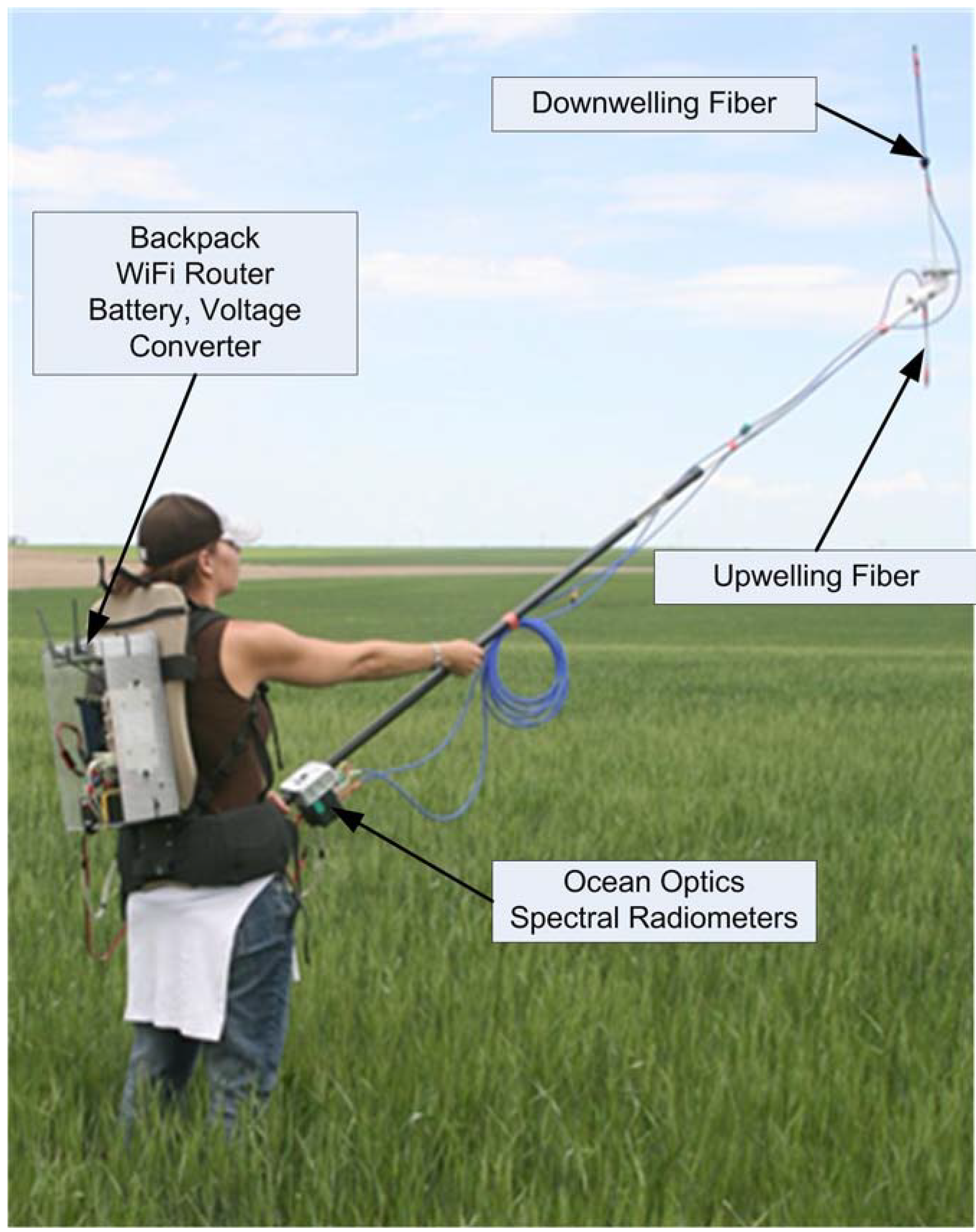
3.2. Acquiring Spectral-Reflectance Data at Canopy and Plant Community Levels: The Human-Transported Backpack Sensor System

In our field configuration, depicted as the block diagram in Figure 2, all of the elements, except for the computer, are mounted in a self-contained backpack which includes: (1) an inexpensive WiFi router for the computer connection; (2) a serial terminal server to convert the radiometer serial connection to a TCP/IP network connection; (3) a 12-volt, gel-cell battery; and (4) a voltage converter to provide power to the radiometers. The serial terminal server is the key to separating the instruments from the computer. This device converts RS-232 serial connections to TCP/IP network connections. Driver software on the computer makes this remote connection appear as a local “com port” to application software. Two Ocean Optics 2000 hyperspectral field radiometers (as described above) are mounted on the sensor pole along with the light-collecting fibers. In its original configuration, the serial ports on the Ocean Optics systems are interconnected to the backpack using two RS-232 serial cables. In current versions, the Ocean Optics USB interfaces are connected to a USB terminal server.

As can be seen in Figure 3, there are several distinct advantages to the configuration. The architecture protects the collection fibers since they are attached only to the pole and to the pole-mounted radiometers. The use of a wireless router means that the computer can be conveniently located within a 300-meter radius from the sensor pole. Because all of the equipment is integrated onto the pole and into the backpack, there are only three connectors (two serial and one power) that need to be attached during equipment setup. Note that excess fiber is coiled and attached to the mounting pole. The amount of excess fiber does not affect the quality of the data taken and facilitates using different mounting configurations when needed.

In concert with the development of the backpack, a similar packaging architecture was applied to instruments used for limnological studies (e.g., assessing the quality of surface waters).

Figure 2. Block diagram of backpack components.

Figure 2. Block diagram of backpack components.

Figure 3. Wireless instrument backpack and instrument pole. Note the up- and down-welling fibers at the end of the pole and the spectral radiometers at its base.

Figure 3. Wireless instrument backpack and instrument pole. Note the up- and down-welling fibers at the end of the pole and the spectral radiometers at its base.

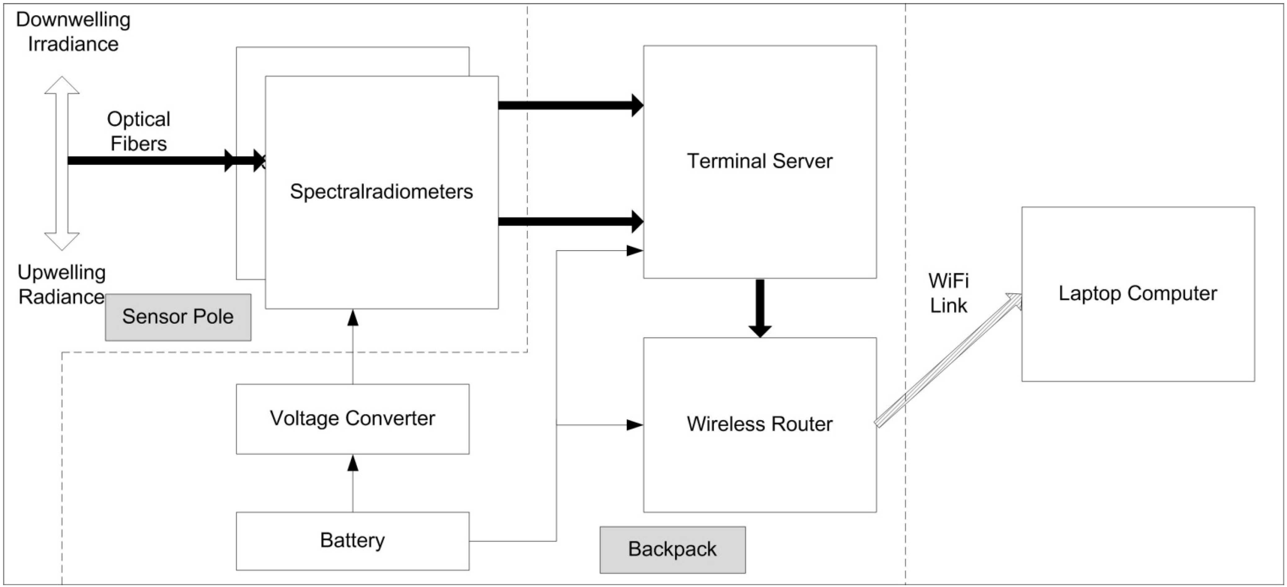
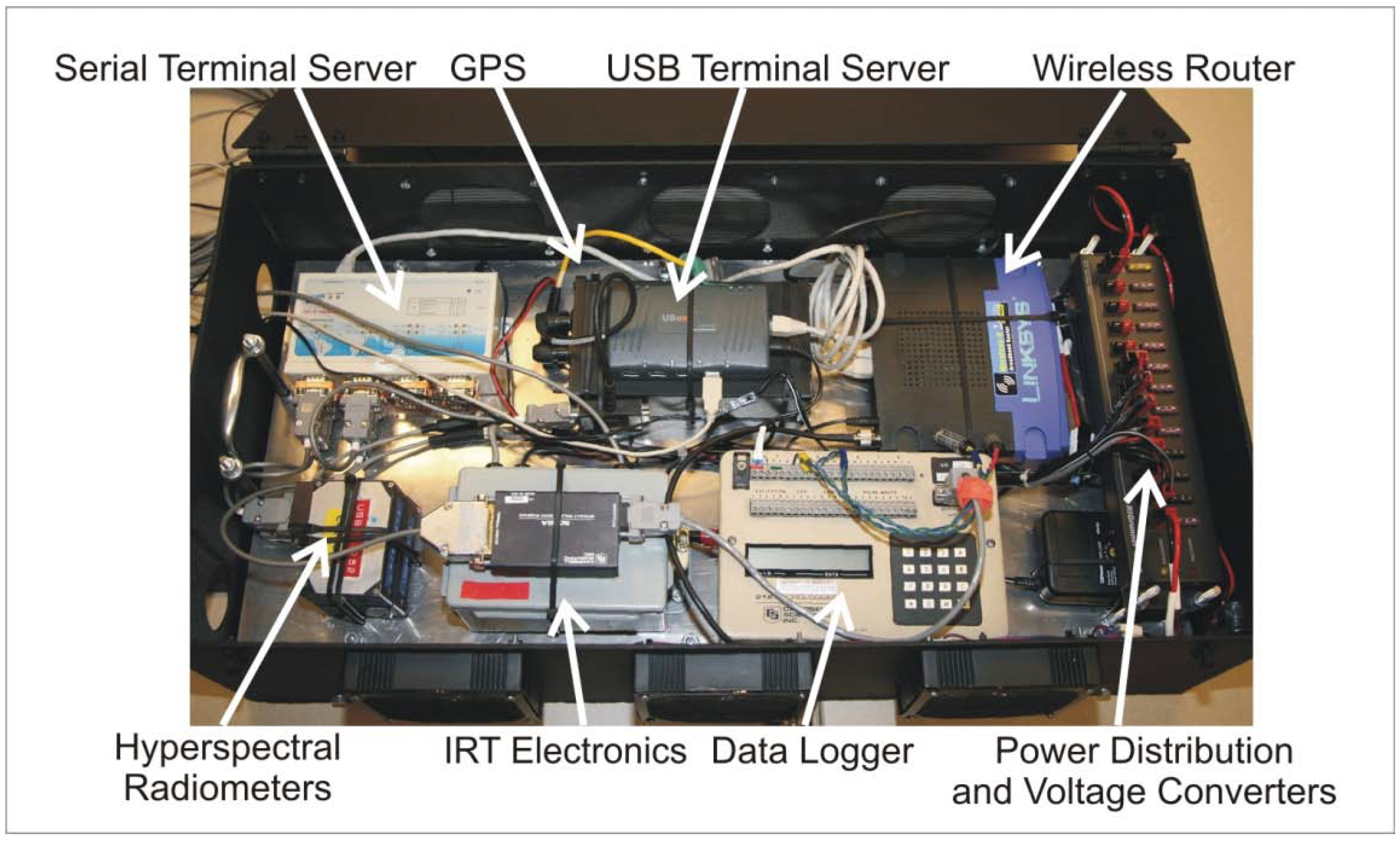
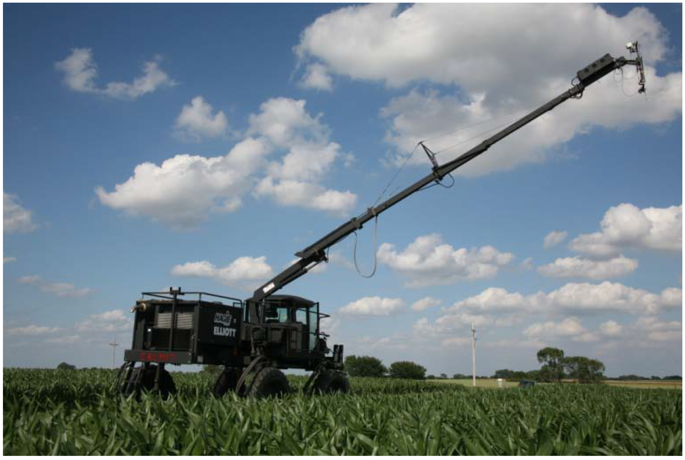
3.3. Acquiring Spectral-Reflectance Data at Canopy and Plant Community Levels: The Hercules Motorized-Vehicle System with Wireless Communications

In 2008, the research team created a versatile, all-terrain platform, affectionately known as “Hercules,” to facilitate in-situ data collection in a repeatable, scientifically valid manner (Figure 4). It constituted an attempt to address all of the necessary considerations and procedures for collecting science quality spectral data (summarized in Section 2.0). The platform is based upon the successes achieved with an earlier version of an all-terrain motorized platform [8]. The base tractor for Hercules was the prototype used in the development of the Hagie (Clarion, IA, USA) STS series of self-propelled spray coupes. A rear-mounted 365 hp turbocharged Cummins diesel engine powers a joystick-controlled, 3-speed, hydrostatic 4-wheel-drive propulsion system. Hercules is capable of reaching speeds of 45 kph, which greatly enhances research productivity because no trailer is needed to travel between research fields.

Figure 4. The Hercules research platform shown was configured for making hyperspectral observations. The self-leveling sensor frame is seen at the upper right. The frame includes up- and down-welling optical fibers, GPS antenna, infrared thermometer, pyranometer, quantum sensor, and down-looking digital camera. The Hercules Instrument Box is located just to the left and below the sensor frame.

Figure 4. The Hercules research platform shown was configured for making hyperspectral observations. The self-leveling sensor frame is seen at the upper right. The frame includes up- and down-welling optical fibers, GPS antenna, infrared thermometer, pyranometer, quantum sensor, and down-looking digital camera. The Hercules Instrument Box is located just to the left and below the sensor frame.

Hercules weighs nearly 9000 kg and is 3.7 m wide, 3.5 m high, and 7.6 m in length. It has a turn radius of 5.5 m and under-frame clearance of 1.8 m, which facilitates data collection in tall, late-season crops.

Instruments for data collection are deployed on a center-mounted boom located immediately behind the cab (Figure 4). Multiple hydraulically activated articulation points and a full 360-degree swing arc enable the operator to position an instrument package in a range of heights from centimeters above the ground to approximately 12.8 m at maximum extension. The main boom section (6.4 m long) has a maximum lifting capacity of about 454 kg. A manually extendable, multi-position jib of 6.4 m is available for adding length to the boom, but reduces the payload to 68 kg. Other assorted features include remote boom control (within 152 m), adjustable tread width (3 m to 4 m), and independent air-ride suspension between cab and payload platform.

The electronics and instrumentation configuration on Hercules builds on experience gained with “Goliath,” the earlier, smaller, machine, which had many cables running up and down the support boom in order to interconnect instruments and the control/data acquisition computer. Despite care taken when clamping and positioning them, there was a high probability that cables would be pinched, or even severed, as the boom was extended or rotated. The instruments on Goliath were shared with other experimenters; hence connectors were mated and separated at least weekly leading to physical damage due to wear and bent pins. Goliath was also equipped with a ruggedized desktop computer. Long exposure to sun and high levels of vibration damaged adapters and hard drives in that machine.

The instruments and electronics on Hercules were, like the backpack described earlier, integrated into the “Hercules Instrument Box” (HIB), and connected via WiFi technology with a cab-mounted computer (or a laptop in the field, as needed) Figure 4 depicts the instrument boom positioned to acquire data. The end of the boom has a self-righting frame which holds the upwelling and downwelling light-collecting fibers, a GPS antenna, a down-looking infrared thermometer (IRT), a downwelling global-irradiance pyranometer, a downwelling PAR quantum sensor, and a down-looking camera to photograph the scene in the upwelling fiber field of view (25°). The fibers and electrical interconnections to the instruments are routed from the frame to the HIB, mounted on the boom just below the frame. A ruggedized power cable is the only physical electrical connection running up the boom.

The electronics inside the HIB are shown in Figure 5. As described for the backpack, a serial terminal server provides physical serial ports within the HIB and corresponding virtual ports via a TCP/IP network to the controlling computer. In addition, the HIB contains a USB terminal server that performs an analogous function for devices using USB connectivity. Application software cannot distinguish these virtual ports from the conventional hardware ports. Hence, no modifications are required to instrument-control and data-acquisition software in order to remotely connect to instruments. The terminal server provides USB connectivity for the down-looking digital camera. The serial terminal server supports several instruments including Ocean Optics hyperspectral field radiometers, GPS, and Campbell data logger (Logan, UT, USA). The data logger collects information sent from the pyranometer, quantum sensor, and IRT. The terminal servers are connected via short Ethernet cables to an inexpensive wireless router. Two external antennas connect to the router in order to assure good signal strength to the laptop computer (normally operated in the Hercules cab).

The HIB also includes a 12-volt distribution block and voltage converters for 6 and 5 volts. These lower voltages are required to power the radiometers and the digital camera. Three fans provide cooling air flow to keep the instruments within the limits of their operating temperatures.

The digital camera, while primarily used as a scene capture and documentation device, also helps position the Hercules boom. A software reticule is superimposed on the computer-screen display of an image captured by the nadir-looking boom camera to help set the boom height. The reticule has rotatable and positionable parallel lines spaced so that when the lines overlay the rows of a crop, the upwelling fiber on the boom is 16 feet above the canopy. The reticule spacing may be adjusted by the operator if other heights are required or if crop row spacing varies.

Figure 5. Hercules Instrument Box (HIB) and components.

Figure 5. Hercules Instrument Box (HIB) and components.

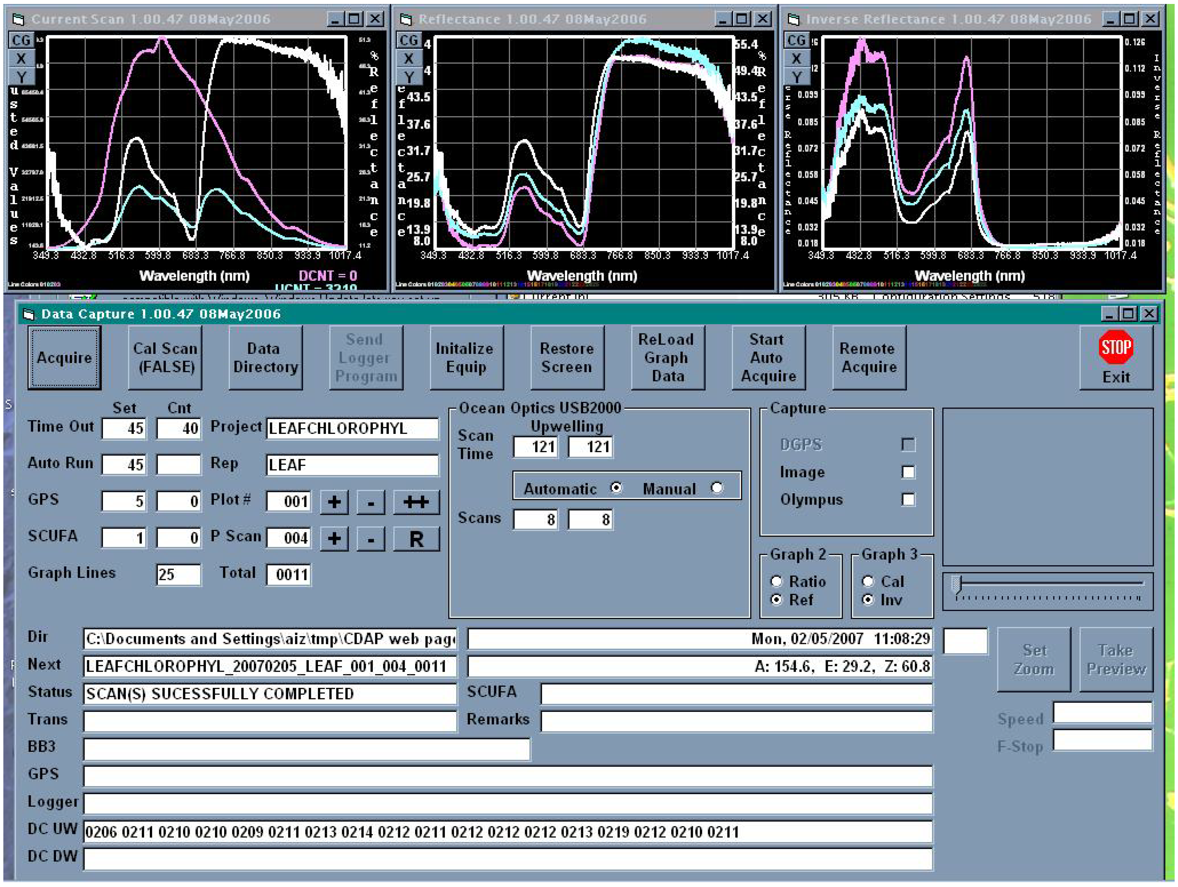
4. The Data-Collection, Processing, and Display Software

A very important and unique component of our system is the CALMIT Data Acquisition Program (CDAP^TM), developed to support field spectral data collection by operating and collecting data from numerous types of hyperspectral field radiometers and ancillary instruments such as pyranometers, GPS, etc. An outstanding characteristic of the CDAP software is that it provides for immediate viewing of acquired spectra and ancillary data. Thus, field personnel can assess the quality of their data acquisitions, as well as crop status, before proceeding to other locations in a field.

The program also performs post-processing on collected data to create tab-delimited files containing spectra, calculated reflectance, and ancillary instrument data that may be easily imported into spreadsheet software, such as Excel, or into special purpose software written in virtually any programming language. This facilitates the near-real time monitoring of key biophysical characteristics such as fraction of green vegetation (VF), fraction of absorbed photosynthetically active radiation (fAPAR), green leaf area index (GLAI), and biomass, among others. To better understand this software, the following paragraphs describe the phases and modes of using CDAP.

4.1. Equipment Configuration

CDAP’s configuration files are pre-set to contain operating parameters, serial numbers, and other information to define the appropriate operating conditions for all instruments and to initialize their operating state. The software can also be set to support single-head (one radiometer) or dual-head operation (two radiometers to capture both upwelling and downwelling radiation simultaneously). Parameters modeling the characteristics of reflective reference panels are included to correctly provide a full-brightness baseline during calibration.

4.2. Operating—Data Acquisition

Upon completion of system configuration, CDAP begins collecting GPS and data logger data streams, and saving them to files. Whether in calibration or observation mode, CDAP configures the radiometers and takes an initial spectral scan to determine incoming downwelling irradiance and to appropriately set instrument integration times. Once set, CDAP performs a spectral scan and writes the data obtained to a file. At the same time, if so selected, CDAP executes a shutter trigger command to the digital camera in order to capture the scene in the radiometer field of view. The program is equipped to automatically download data from the camera or to retrieve the picture file from a directory if camera software controls the download. In the calibrating and observing modes, CDAP provides to the operator both real-time quick-look reflectance and (quasi) absorption spectra (Figure 6), as well as camera images. The operator can use this information to ascertain correct operation and equipment configuration.

Figure 6. This screen capture shows CALMIT Data Acquisition Program (CDAP^TM) during field observation. The graphs at the top show, left to right, the upwelling radiance and downwelling irradiance; calculated reflectance and reciprocal reflectance (a proxy of absorbance). The last 25 observations are plotted on the right two screens. The plots are colorcoded with the latest being bright white to distinguish them. Operating parameters and activating buttons are shown in the control screen. The panel at the right center can contain a camera image preview. The lower part of the screen shows raw data and the status of data collection.

Figure 6. This screen capture shows CALMIT Data Acquisition Program (CDAP^TM) during field observation. The graphs at the top show, left to right, the upwelling radiance and downwelling irradiance; calculated reflectance and reciprocal reflectance (a proxy of absorbance). The last 25 observations are plotted on the right two screens. The plots are colorcoded with the latest being bright white to distinguish them. Operating parameters and activating buttons are shown in the control screen. The panel at the right center can contain a camera image preview. The lower part of the screen shows raw data and the status of data collection.

Prior to actual data collection, a Spectralon (North Sutton, NH, USA) 99% reflective reference panel is positioned beneath the sensor and scanned in order not only to assure that both Ocean Optics radiometers are spectrally coincident (levels of sensitivity as well as band centers) but also to link all subsequent measurements of downwelling irradiance to national standards (via the documented characteristics of the reference surface). The median reflectance spectrum from the Spectralon panel is adjusted as required based on the manufacturer’s coefficients that describe the spectral reflectivity of the panel at a given wavelength. All other calibration is based upon the simultaneous measurement of upwelling radiance and downwelling irradiance. The procedure, as described in Rundquist [8] (and in preceding text), involves Radiometer #1, equipped with a 25° field-of-view optical fiber being pointed downward to measure the radiance upwelling from the crop canopy (L_λ^maize). Radiometer #2, equipped with an optical fiber and cosine diffuser (yielding a hemispherical field of view), is pointed upward to simultaneously measure incident irradiance (E_λ^inc). To match their transfer functions, the inter-calibration of the radiometers is accomplished by measuring the upwelling radiance (L_λ^cal) of the white Spectralon reflectance standard, simultaneously with incident irradiance (E_λ^cal). Percent reflectance, ρ_λ, is computed as:

(1)

One critical issue with regard to the dual-fiber approach is that the transfer functions of both radiometers must be identical. We tested our Ocean Optics instruments under laboratory and field conditions and found that over a four-hour period the coefficient of variation of the ratio of the two transfer functions did not exceed 0.4%.

During operation, CDAP may be configured to operate in a manual mode or an automatic mode where measurements are taken repeatedly at a specified rate. CDAP has been successfully used in diverse field venues for several years. The combination of real-time quick-look and integrated raw observation files has provided a robust experiment environment. CDAP is available for licensing from the University of Nebraska.

5. Algorithms and Standard Products for Inferring Crop-Biophysical Characteristics

Once field data are collected, the processing algorithm, designed to ingest massive amounts of data in an efficient and systematic manner, is invoked. The procedures are based on standardized macros and three basic “levels” of data-handling/analyses. During Level-1 processing, the raw spectral data are converted to percent reflectance, stored in an Excel spreadsheet, interpolated at a 1-nm interval, and compressed for archiving purposes. At this stage, mean values of reflectance for each sampled area and the standard deviations of reflectance are calculated and, thus, these statistics characterize each sampled area.

Level-2 processing involves integration of Ocean Optics reflectance to simulate informative spectral regions for retrieval of crop biophysical characteristics including spectral bands of our own airborne AISA-Eagle scanner as well as existing space borne systems (e.g., TM Landsat, MODIS, MERIS). The final processing step, Level-3, addresses the estimation of biophysical and agronomic characteristics of crops using a developed suite of algorithms, as described below.

Our suite of algorithms includes procedures for retrieval of (i) foliar pigment content including total chlorophyll, carotenoids, and anthocyanins [13,14,15] and (ii) crop biophysical characteristics including vegetation fraction (VF), fraction of photosynthetically active radiation absorbed by live vegetation (fAPAR_green) [16], green LAI, green leaf biomass, and gross primary production (GPP).

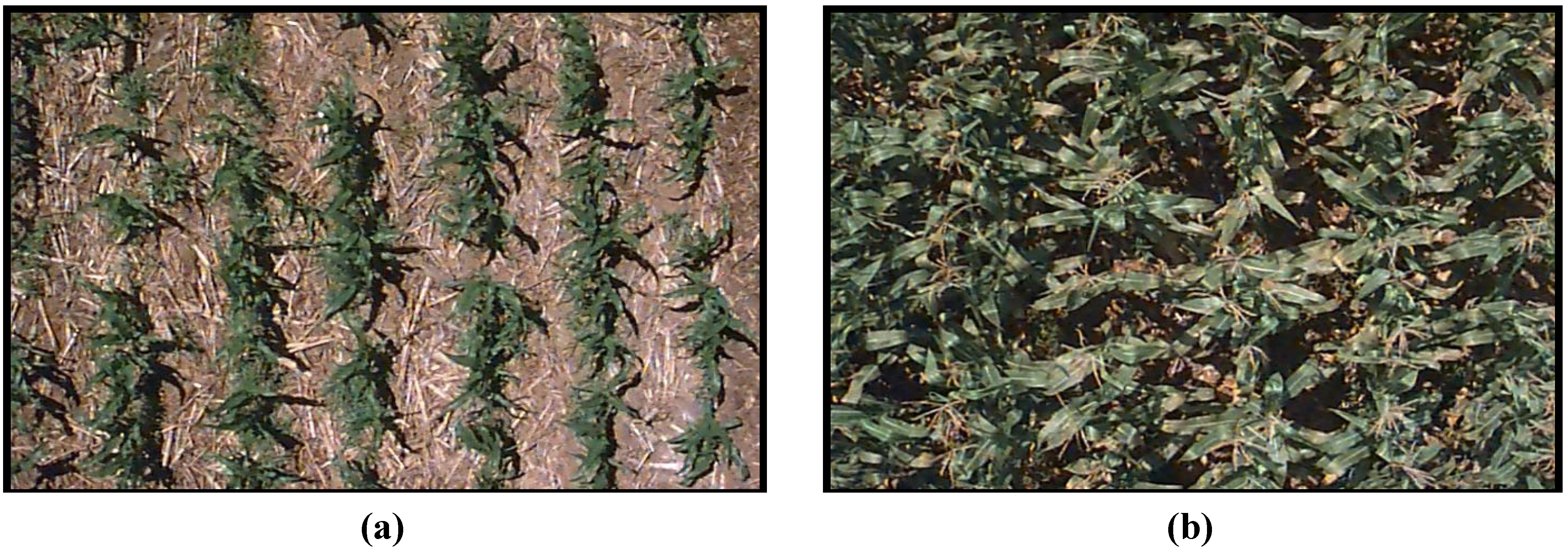
5.1. Vegetation Fraction (VF)

VF is useful as an indicator of not only crop phenological status but also of final crop yield. Reflectances in only the visible range of the spectrum have been used to quantitatively estimate VF. For close-range sensing, we use the modified Visible Atmospherically Resistant Vegetation Index (VARI) with a red (660–680 nm) band and bands in the either green (540–560 nm) or red edge (700–710 nm) region [17]:

mVARI_green = (ρ_green − ρ_red)/(ρ_green + ρ_red)

(2)

mVARI_{red edge} = (ρ_{red edge} − ρ_red)/(ρ_{red edge} + ρ_red)

(3)

To make the indices resistant to atmospheric effects, a blue spectral band was employed [17]:

VARI_green = (ρ_green − ρ_red)/(ρ_green + ρ_red − ρ_blue)

(4)

VARI_{red edge} = (ρ_{red edge} − 1.7ρ_red + 0.7ρ_blue)/(ρ_{red edge} + 2.3ρ_red − 1.3ρ_blue)

(5)

where ρ_blue is in the range 470–480 nm, ρ_green is in the range 540–560 nm, ρ_{red edge} in the range 700–710 nm, The error in estimating VF using VARI has been documented to be less than 10% [17,18].

The VARI was also used for evaluation the phenological development of maize [18], and it allowed for the identification of the timing of phenological transitions that are related with the maize physiological development. The index also allowed identification of the onset of the grain fill period, which is important since maximum yield potential of maize plants depends on optimal environmental conditions during this period.

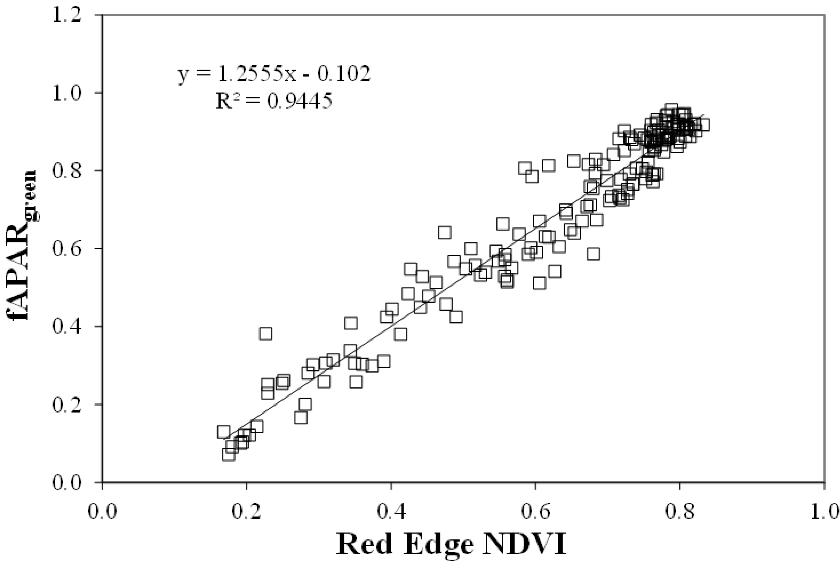
5.2. Fraction of Absorbed Photosynthetically Active Radiation (fAPAR_green)

The estimation of fraction of radiation absorbed by green photosynthetically active vegetation (fAPAR_green) was accomplished by using either green or red edge Normalized Difference Vegetation Index (NDVI) in the following forms [19]:

Green NDVI = (ρ_NIR − ρ_green)/(ρ_NIR + ρ_green)

(6)

Red Edge NDVI = (ρ_NIR − ρ_{red edge})/(ρ_NIR + ρ_{red edge})

(7)

where ρ_green is in the range 540–560 nm, ρ_{red edge} in the range 700–710 nm, and ρ_NIR in the range 840–870 nm. We have also used the Wide Dynamic Range Vegetation Index [20], in the form:

WDRVI = (aρ_NIR − ρ_red)/(aρ_NIR + ρ_red)

(8)

with the weighting coefficient a = 0.2.

These indices were related to fAPAR_green [18] with a coefficient of determination greater than 0.91, and were able to estimate fAPAR_green in the range 0 through 0.95 with root mean square errors less than 0.072 (Green NDVI), 0.071 (WDRVI), and 0.057 (Red Edge NDVI, Figure 7) [21].

Figure 7. Relationship between red-edge NDVI and fAPAR_green for maize and soybean. Regression line is significant at the 0.01 level.

Figure 7. Relationship between red-edge NDVI and fAPAR_green for maize and soybean. Regression line is significant at the 0.01 level.

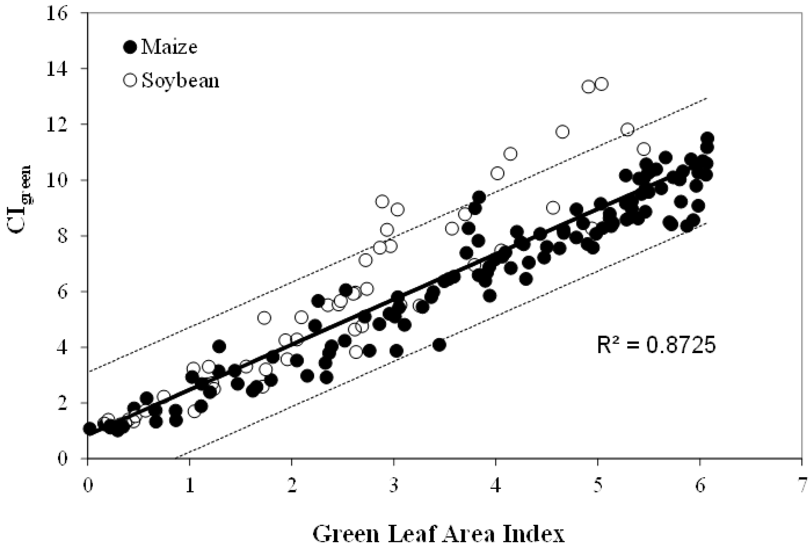
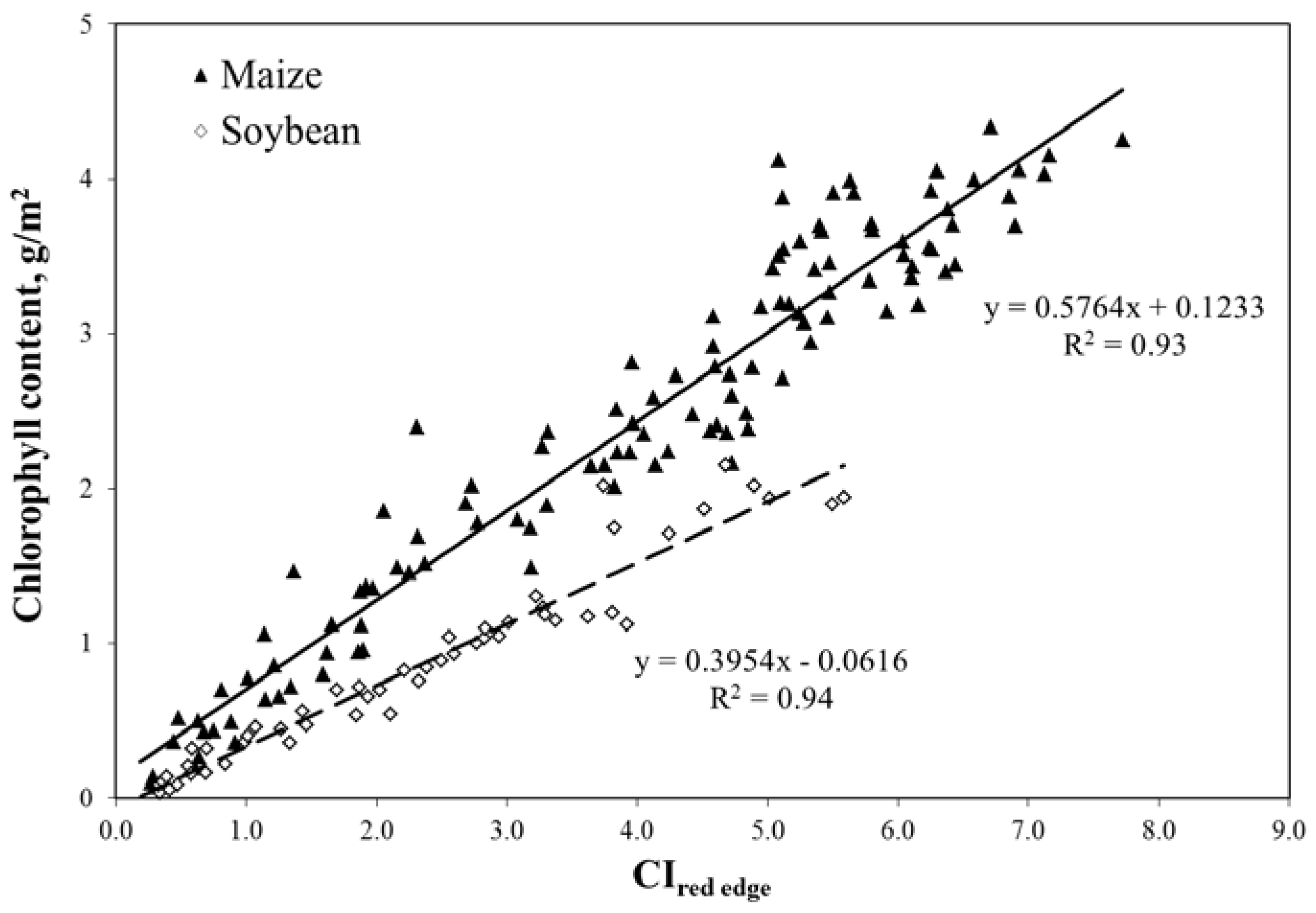
5.3. Green Leaf Area Index (LAI), Green Leaf Biomass and Chlorophyll Content

The LAI, chlorophyll content and biomass are important crop biophysical characteristics used for climate modeling, estimating primary production, and forecasting crop yield. All three of these biophysical characteristics are related, and can be estimated remotely using different parameterization of chlorophyll indices (CI) [22,23]:

CI_green = (ρ_NIR/ρ_green) − 1

(9)

CI_{red edge} = (ρ_NIR/ρ_{red edge}) − 1

(10)

where reflectances ρ_NIR, ρ_green and ρ_{red edge} are in spectral bands as in Equations (5) and (6).

The algorithms for LAI and green leaf biomass estimation, summarized by Gitelson et al. [22] and Vina et al. [21] have been calibrated in maize and soybean for LAI ranging from 0 to more than 6 (Figure 8) and for leaf biomass up to 3500 kg/ha. Validation using independent data sets showed that algorithms allowed accurate estimation of LAI and green biomass. They were able to estimate green LAI with RMSE below 0.51 m²/m² (CI_green) and 0.37 m²/m² (CI_{red edge}) and biomass below 242 kg/ha [22].

The same models as in Equations (9) and (10) were parameterized for accurate remote assessment of total canopy chlorophyll content in crops [23] that brings users a quantitative measure of crop greenness, as shown in Figure 9. When the red edge band was selected (720–730 nm), CI_{red edge} became non-species-specific and, thus, the algorithm for chlorophyll content estimation did not require re-parameterization for the diverse canopy and leaf structures seen in C3 and C4 crops such as maize and soybean [23]. Using the close relationship between crop total canopy chlorophyll content and gross primary production (GPP) [13], we developed a technique for remote estimation of GPP.

Figure 8. Green chlorophyll index (CI_green) plotted versus green LAI in irrigated and rainfed maize and soybean.

Figure 8. Green chlorophyll index (CI_green) plotted versus green LAI in irrigated and rainfed maize and soybean.

Figure 9. Red edge chlorophyll index (CI_{red edge}) in the MERIS spectral bands plotted versus total canopy chlorophyll content in irrigated and rainfed maize and soybean [23].

Figure 9. Red edge chlorophyll index (CI_{red edge}) in the MERIS spectral bands plotted versus total canopy chlorophyll content in irrigated and rainfed maize and soybean [23].

In addition to these indices, useful in estimating chlorophyll content, analogous indices have been developed to estimate other pigment content including carotenoids and anthocyanins [15,24].

6. Conclusions

The unique system described in this paper comprises a powerful approach to systematic collection of science quality data, innovative analyses, and the development of practical products. The system includes solutions to acquisition of spectral data for vegetation in the field at canopy level. Our approach generates the estimation of foliar pigment contents (chlorophyll, carotenoids, and anthocyanins) and the following biophysical characteristics: green vegetation cover, fraction of absorbed photosynthetically active radiation, green LAI, green leaf biomass, total canopy chlorophyll content, and gross primary production. It should be noted that the suite of algorithms has been used successfully to estimate crop biophysical characteristics from, not only close-range in the field (and at leaf level in the lab), but also from aircraft altitudes using the UNL/CALMIT AISA-Eagle imaging spectrometer. Our system has been routinely used and tested over a period of more than ten years with great success. It also allows us to monitor different but interrelated crop biophysical characteristics that were formerly represented by only one index (namely NDVI). An outstanding attribute of the system is that it not only facilitates research but also yields useful products for agriculture.

References

1. Pinter, P., Jr.; Hatfield, J.; Schepers, J.; Barnes, E.; Moran, M.; Daughtry, C.; Upchurch, D. Remote sensing for crop management. Photogramm. Eng. Remote Sens. 2003, 69, 647–664. [Google Scholar] [CrossRef]
2. Nicodemus, F.; Richmond, J.; Hsia, J.; Ginsberg, I.; Limperis, T.; Ott, W. Geometrical Considerations and Nomenclature for Reflectance; US Department of Commerce, National Bureau of Standards: Washington, DC, USA, 1977. [Google Scholar]
3. Duggin, M. Simultaneous measurement of irradiance and reflected radiance in field determination of spectral reflectance. Appl. Opt. 2005, 20, 3816–3818. [Google Scholar] [CrossRef]
4. Duggin, M.; Philipson, W. Field measurement of reflectance: Some major considerations. Appl. Opt. 1982, 21, 2833–2840. [Google Scholar] [CrossRef]
5. Milton, E. Does the use of two radiometers correct for irradiance changes during measurements. Photogramm. Eng. Remote Sens. 1981, 47, 1223–1225. [Google Scholar]
6. Milton, E.; Schaepman, M.; Anderson, K.; Kneubühler, M.; Fox, N. Progress in field spectroscopy. Remote Sens. Environ. 2009, 113, S92–S109. [Google Scholar] [CrossRef]
7. Milton, E. Principles of field spectroscopy. Int. J. Remote Sens. 1987, 8, 1807–1827. [Google Scholar] [CrossRef]
8. Rundquist, D.; Perk, R.; Leavitt, B.; Keydan, G.; Gitelson, A. Collecting spectral data over cropland vegetation using machine positioning versus hand-held positioning of the sensor. Comput. Electron. Agric. 2004, 43, 173–178. [Google Scholar] [CrossRef]
9. Anderson, K.; Milton, E.; Rollin, E. Calibration of dual-beam spectroradiometric data. Int. J. Remote Sens. 2006, 27, 975–986. [Google Scholar] [CrossRef]
10. Dall’Olmo, G.; Gitelson, A.A. Effect of bio-optical parameter variability on the remote estimation of chlorophyll-a concentration in turbid productive waters: Experimental results. Appl. Opt. 2005, 44, 412–422. [Google Scholar] [CrossRef]
11. Meyer, G.E.; Hindman, T.; Lakshmi, K. Machine Detection Parameters for Plant Species Identification. In Precision Agriculture and Biological Quality; Meyer, G.E., DeShazer, J.A., Eds.; The International Society for Optical Engineering: Boston, MA, USA, 1998; pp. 327–335. [Google Scholar]
12. Vina, A.; Gitelson, A.; Rundquist, D.; Keydan, G.; Leavitt, B.; Schepers, J. Monitoring maize (Zea mays L.) phenology with remote sensing. Agron. J. 2004, 96, 1139–1147. [Google Scholar] [CrossRef]
13. Gitelson, A.A.; Viña, A.; Verma, S.B.; Rundquist, D.C.; Arkebauer, T.J.; Keydan, G.; Leavitt, B.; Ciganda, V.; Burba, G.G.; Suyker, A.E. Relationship between gross primary production and chlorophyll content in crops: Implications for the synoptic monitoring of vegetation productivity. J. Geophys. Res. 2006, 111, D08S11. [Google Scholar] [CrossRef]
14. Steele, M.; Gitelson, A.A.; Rundquist, D. Non-destructive estimation of leaf chlorophyll content in grapes. Am. J. Enol. Vitic. 2008, 59, 299–305. [Google Scholar]
15. Steele, M.R.; Gitelson, A.A.; Rundquist, D. Non-destructive estimation of anthocyanin content in grapevine leaves. Am. J. Enol. Vitic. 2008, 60, 87–92. [Google Scholar]
16. Hall, F.G.; Huemmrich, K.F.; Goetz, S.J.; Sellers, P.J.; Nickeson, J.E. Satellite remote sensing of surface energy balance: Success, failures and unresolved issues in FIFE. J. Geophys. Res. 1992, 97, 19061–19089. [Google Scholar] [CrossRef]
17. Gitelson, A.; Kaufman, Y.; Stark, R.; Rundquist, D. Novel algorithms for remote estimation of vegetation fraction. Remote Sens. Environ. 2002, 80, 76–87. [Google Scholar] [CrossRef]
18. Viña, A.; Gitelson, A.A. New developments in the remote estimation of the fraction of absorbed photosynthetically active radiation in crops. Geophys. Res. Lett. 2005, 32, L17403. [Google Scholar] [CrossRef]
19. Gitelson, A.; Kaufman, Y.; Merzlyak, M. Use of a green channel in remote sensing of global vegetation from EOS-MODIS. Remote Sens. Environ. 1996, 58, 289–298. [Google Scholar] [CrossRef]
20. Gitelson, A.A. Wide dynamic range vegetation index for remote quantification of crop biophysical characteristics. J. Plant Physiol. 2004, 161, 165–173. [Google Scholar] [CrossRef]
21. Viña, A.; Gitelson, A.A.; Nguy-Robertson, A.L.; Peng, Y. Comparison of different vegetation indices for the remote assessment of green leaf area index of crops. Remote Sens. Environ. 2011, 115, 3468–3478. [Google Scholar] [CrossRef]
22. Gitelson, A.; Vina, A.; Arkebauer, T.; Rundquist, D.; Keydan, G.; Leavitt, B. Remote estimation of leaf area index and green leaf biomass in maize canopies. Geophys. Res. Lett. 2003, 30, 1148. [Google Scholar] [CrossRef]
23. Gitelson, A.A.; Viña, A.; Rundquist, D.C.; Ciganda, V.; Arkebauer, T.J. Remote estimation of canopy chlorophyll content in crops. Geophys. Res. Lett. 2005, 32, L08403. [Google Scholar] [CrossRef]
24. Gitelson, A.A.; Keydan, G.P.; Merzlyak, M.N. Three-band model for noninvasive estimation of chlorophyll carotenoids and anthocyanin contents in higher plant leaves. Geophys. Res. Lett. 2006, 33, L11402. [Google Scholar] [CrossRef]