Article

Numerical Simulation of Soil Water–Salt Dynamics and Agricultural Production in Reclaiming Coastal Areas Using Subsurface Pipe Drainage

College of Hydraulic Science and Engineering, Yangzhou University, Yangzhou 225009, China
*
Author to whom correspondence should be addressed.
Agronomy 2023, 13(2), 588; https://doi.org/10.3390/agronomy13020588
Submission received: 3 January 2023 / Revised: 9 February 2023 / Accepted: 16 February 2023 / Published: 18 February 2023

Abstract

:
Soil salinization induced by shallow saline groundwater in coastal areas can be managed using subsurface pipe drainage (SPD) for agricultural land reclamation. However, a reasonable SPD system layout should comprehensively consider local hydrological conditions and crop physiological characteristics based on long-term model evaluations. The objectives of this study were to test the applicability of a crop growth model (AquaCrop) for simulating winter wheat growth in SPD-applied fields by employing the water table behaviors predicted by the soil hydrologic model HYDRUS. Model calibration and validation based on field observations suggested that HYDRUS accurately predicted the distributions of soil water–salt dynamics, and the seasonal variations of canopy cover and biomass production predicted by AquaCrop were close to the measured values. The simulation scenarios considering the long-term effect of groundwater salinity (10.53, 21.06, and 31.59 g L−1 for low, medium, and high levels), drain spacing (10, 20, 30, 40 m, and no-SPD), and precipitation category (dry, normal, and wet year) on soil solute transport, grain yield (GY), water productivity (WP), and groundwater supply (GS) were further explored using a combination of HYDRUS and AquaCrop. The simulation results indicated that narrowing the drain spacing could improve the desalination performance of SPD, but there was no continuous downward trend of soil solute concentration during the long-term application of SPD when groundwater salinity was constant. The SPD application could improve grain yield by 0.81–1.65 t ha−1, water productivity by 0.13–0.35 kg m−3, and groundwater supply by 6.06–31.03 mm compared to the no-SPD scenarios, but such increases would be less pronounced in dry years with groundwater salinity at the low level. This study demonstrated that the co-application of hydrologic and crop growth models is a feasible method for revealing the effects of SPD on agricultural land reclamation in coastal areas.

1. Introduction

By the end of the 21st century, the global extent of coastal marshes is predicted to increase by 60% compared to the current area (approximately 2 × 10⁵ km2), under the present level of fluvial sediment supply [1]. Therefore, coastal land reclamation is widely regarded as a sustainable strategy for meeting the increasing land resource demand for urbanization, industrialization, and agriculture [2]. However, the hydrological and hydrochemical conditions in the freshwater–seawater-interacting coastal stratum are controlled by land–ocean hydraulic gradients [3,4], which are likely to induce seawater intrusion and cause soil salinization in low-lying terrain (such as salt marshes or mudflats), which is often considered to be land resources reserved for cultivation [5]. The salinity dynamics in the soil surface layer of the coastal area are affected by precipitation, phreatic water evaporation, surface ecosystems, topography, and seawater intrusion [6,7,8], but the root cause of soil salinization is capillary-driven upward solute transport from saline groundwater, which may cause salt stress that severely constrains the development of crop-based agriculture when adequate soil leaching and reasonable drainage management are lacking [9].
Subsurface pipe drainage (SPD) has been reported as a suitable method for the desalinization process during land reclamation in coastal areas with a shallow groundwater table and low-permeability soil texture [10,11]. By increasing the lateral discharge of soil water, SPD can control the groundwater table in a timely manner and further limit the capillary-driven upward solute build-up in the upper layers, thereby persistently protecting crop growth from salt stress [12,13]. As numerous previous studies have suggested, the drainage performance of SPD is highly dependent on the layout pattern of the subsurface drainpipe, including drain spacing, buried depth, and drainpipe diameter. The drain spacing can vary from a few to hundreds of meters based on different application requirements, and is the most researched factor during SPD system design [14,15,16]. Reasonable drain spacing usually corresponds to the optimal efficiency of water table control or salt discharge under a specific agricultural condition. Notably, blindly pursuing an SPD with high drainage capacity can induce excessive soil nutrient loss and restricted groundwater supply, which in turn affects crop growth and limits water use efficiency [17]. Therefore, the response of crop growth could be the most intuitive indicator for evaluating land reclamation status under the application of SPD, and the salt dynamics in the soil profile should be analyzed in the long term concerning groundwater salinity and SPD layout patterns.
Multiple factors (e.g., soil properties, weather, crop species, and field management) influence the performance of SPD systems, making it challenging to fully assess their interactions through limited field experimentation. A hydrologic numerical model, HYDRUS, is widely reported to be a powerful tool for integrating various environmental and management factors that influence soil water and solute transport under different SPD system designs [18,19,20]. The HYDRUS model has the advantage of providing flexible boundary conditions and great applicability to variably saturated media, which is convenient for establishing the scenario simulations that take varying rainfall and water table behaviors into account [21]. Additionally, the HYDRUS model uses an osmotic-pressure-related equation to calculate root water uptake [22], and incorporates a compensatory mechanism for the simulation of root-level physiological responses subject to salt and water stress situations [23]. However, the HYDRUS model lacks the ability to predict stress-affected crop biomass development and final grain yield, limiting the model application prospect in the evaluation of land reclamation for agricultural purposes. Therefore, the HYDRUS model has been recommended to be co-applied with crop growth models such as WOFOST, DSSAT, and AquaCrop to predict the crop development in fields with particular fertilization or irrigation regimes [24,25,26]. In terms of the crop-based model, the canopy-level AquaCrop model, based on the conservative relationship between crop biomass and transpiration, has been extensively studied to guide field-scale water or fertilizer management by estimating crop biomass progression, grain yield, and associated water productivity [27,28,29]. Meanwhile, in AquaCrop, the effect of soil salinity on biomass production is described by a salinity stress–crop response curve which consists of a lower and an upper threshold of soil salt content that corresponds to the extent of salt stress from no effect to full effect [30]. However, the drainage process in the soil profile is simplified in AquaCrop and is uniformly classified as deep percolation [31], which causes AquaCrop to be unable to calculate the lateral flow in drained fields or further simulate water table behaviors affected by SPD [32,33]. So far, AquaCrop has not been combined with HYDRUS to simulate the crop growth response to SPD in a coastal reclamation area where soil salinization is mainly caused by capillary-raised solutes from saline groundwater.
Thus, the main objectives of this study were to: (1) verify the feasibility of the AquaCrop model for simulating the response of crop growth in SPD-applied fields based on HYDRUS-predicted water table behaviors; (2) explore the evolution of soil solute concentration under long-term (30 years) application of the SPD system; and (3) investigate the variability of crop grain yield, water productivity, and groundwater upward supply as a function of groundwater salinity and drain spacing in different precipitation years.

2. Materials and Methods

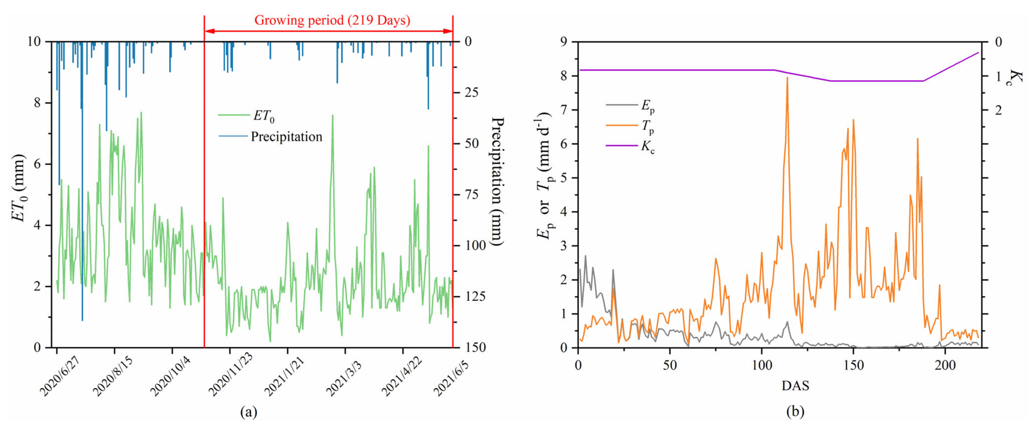
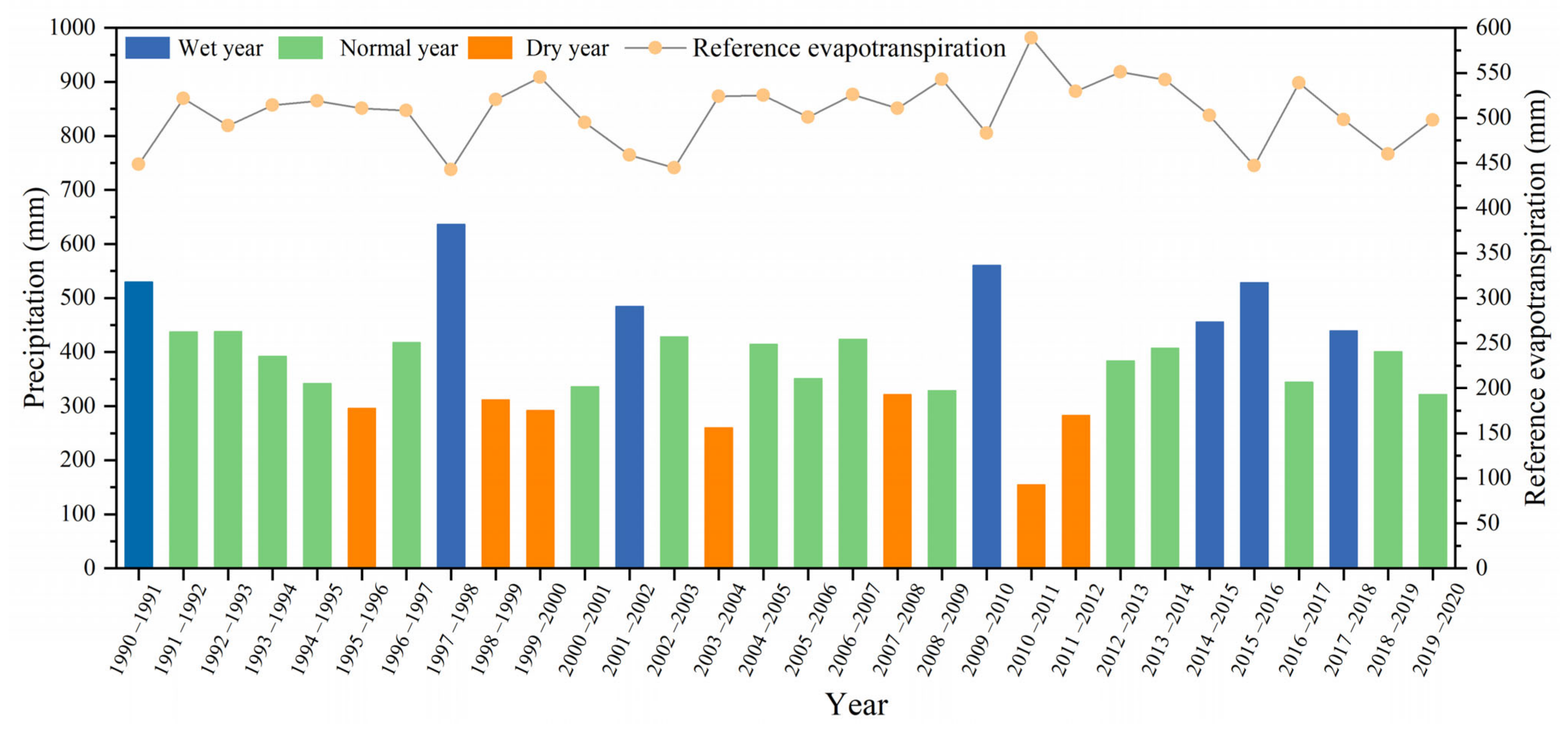
2.1. Experimental Site Description and Data Collection

This study was conducted from 2020 to 2021 at the Coastal Area Research Station of Jiangsu Hydraulic Research Institute, located in Dongtai, Jiangsu Province, Eastern China (120°53′ E, 32°51′ N, mean altitude 4 m above sea level, approximately 5 km away from the Yellow Sea). Formed by sedimentation, the topography in this area is extremely flat (slope ranging from 0.1/1000 to 1/1000), and the dominated land use type is cultivated land for rice and wheat farming. The experimental site has a subtropical monsoon climate, and the long-term average annual air temperature, precipitation, relative humidity, sunshine duration, pan evaporation, and solar radiation are 14.9 °C, 969.2 mm, 79.6%, 1685.5 h, 1064 mm, and 1169 MJ m−1, respectively (meteorological data series of 1953–2020 from the weather station of Dongtai, No. 58251). More than 60% of precipitation is concentrated between June and September. The measured basic physical soil properties at 0–300 cm depth in the experimental field are present in Table 1. The salinity of the 0–300 cm soil profile was averaged at 2.75 dS m−1 (saturated electrical conductivity ECe), which is classified as a slightly saline soil [34].
At the research station (Figure 1), field observations of soil water–salt content and crop growth were conducted in two hydrologically independent rectangular fields (Field A: 80 m × 91 m; Field B: 80 m × 81 m) which were installed with parallel lateral subsurface drainpipes (a perforated plastic pipe of 50 mm diameter). The drain depth of the two fields was set at 0.9 m below the field surface, and the drain spacing was 22.75 and 8.9 m for fields A and B, respectively. The excess soil water collected by the drainpipes of the two fields was uniformly discharged into a nearby collector pond. During the study period, the rain-fed winter wheat (Triticum aestivum L.) variety Ningmai 13 was sown on 30 October 2020 and harvested on 5 June 2021 for both fields. Urea (225 kg ha−1) was combined with 375 kg ha−1 of compound fertilizer (N:P2O5:K2O = 15:15:15) as the base fertilizer, and additional fertilization of 75 kg ha−1 urea and 125 kg ha−1 compound fertilizer was conducted on 24 January 2021, before the winter wheat reviving stage. Other agronomic measures, such as weed control and pest management, were practiced according to local experience.
Observation of soil moisture, salinity, and groundwater table fluctuations in the two fields began simultaneously in June 2020 and ended in July 2021. Soil samples (with five replicates) were obtained using a posthole auger at depths of 20, 50, 80, 110, and 140 cm to test the soil gravimetric water content and soil water electrical conductivity (EC1:5, dS m−1). Groundwater stage gauges (HOBO, U20-001 Onset) were installed in an observation well (depth of 3 m below the soil surface) located at the middle site between two parallel drainpipes to continuously measure the groundwater table variations in each field. Groundwater samples for salinity tests (EC, dS m−1) were monthly collected by a 200-mL cylindrical bucket from three sampling wells (5 cm diameter, 3 m depth) located in the middle position of each field. The canopy cover (CC) and biomass of cultivated wheat were observed at the seedling stage (10 December 2020), tillering stage (1 January 2021), jointing stage (21 March 2021), boot stage (7 April 2021), ripening stage (21 May 2021), and harvest (5 June 2021) for both the two fields. An automatic color threshold image analysis package was used to estimate the CC values [35], and the image resources were captured at five random and non-overlapping observation plots (2 × 2 m for per plot) in each field using a digital camera (Alpha 6400 E18-135 APS-C 24 MP, SONY, Shanghai, China) fixed by a monopod (1.5 m) from the top of the canopy. Five non-adjacent wheat plant areas were selected in each field as the sampling plots (0.5 × 0.5 m per plot) to obtained the in-season aboveground biomass. The field-collected wheat samples were firstly oven-dried at 105 °C for 30 min and then at 75 °C for 48 h to obtain a constant dry weight for biomass measurement.
Weather data, including air temperature, precipitation, solar radiation, wind speed at 2.0 m height, and relative humidity, were recorded hourly by an automatic meteorological station inside the experimental site. Daily reference evapotranspiration (ET0) derived from meteorological data was estimated using an FAO Penman–Monteith method-based ET0 calculator [36]. The variations in precipitation and ET0 during the study period (June 2020 to July 2021) are presented in Figure 2a.

2.2. Model Description

2.2.1. HYDRUS Model

The HYDRUS (2D/3D) software package used in this study is a finite element numerical model that simulates transient or cumulative water and solute transport in variably saturated porous media, based on the two- or three-dimensional form of Richards’ equation [18] and convection–dispersion equation [37]. The van Genuchten–Mualem constitutive relationship was employed in HYDRUS to estimate the soil water retention curve and the unsaturated water conductivity function [38,39].
The model setup of HYDRUS includes geometry establishment, boundary condition selection, and initial condition definition. In this study, a two-dimensional rectangular flow domain was designed for simulating the soil profile (vertical section perpendicular to the drainpipe) for fields A and B. The length of the flow domain corresponded to the actual field size with a depth of 300 cm. As there was no significant difference in soil proprieties within the 30–300 cm soil profile (Table 1), the model domain was divided into 0–30 cm for the surface plough layer and 30–300 cm for the sub-surface layer. The right and left sides of the flow domain were assigned to the no-flux boundary because an impermeable plastic film separated each field at this experimental site. The subsurface drainpipe was modelled by opening a series of 5 cm diameter circular holes on the flow domain at a depth of 90 cm with a horizontal spacing of 22.75 and 8.9 m for fields A and B, respectively. The boundary setting of this model domain is presented in Figure 3. A seepage face was imposed as the boundary condition for these opening holes, simulating the outflow through the drainpipe. An atmospheric boundary condition regarding time-variable rainfall, surface runoff, and evapotranspiration was specified at the soil surface. The bottom boundary was described by a variable pressure head condition, which represented a fluctuating water table (daily field-measured data). Notably, the rise of the field-measured water table is a response to rainfall infiltration, while the atmospheric boundary of HYDRSU also considers the rainfall events, which may accentuate the effect of rainfall events on the simulation results as the model operated under these two boundaries. Therefore, to reduce the water table rise caused by rainfall influencing the simulation of SPD performances, the data of water table depth less than the drain depth (0.9 m) was uniformly adjusted to 0.9 m before setting the bottom boundary condition. Furthermore, the total amount of dissolved salt in rainwater was disregarded because its average EC value was only 0.16 dS m−1. The average groundwater salinity during the investigation period (3.16 g L−1) was set at the bottom boundary to simulate the condition of saline groundwater. The initial conditions within the model domain were imposed by the measured soil water content and salt content at the beginning of the investigation, with a linear variable distribution from the soil surface to the bottom.
Daily potential evapotranspiration (ETp) values derived from the daily ET0 were calculated using crop coefficients at the early (0.7), middle (1.15), and late (0.4) stages of the winter wheat growing season [40] (Figure 2b). The estimated ETp was further separated into potential daily evaporation (Es) and transpiration (Tp) based on the variation in the leaf area index (LAI) [41]. The LAI variations in the studied winter wheat were estimated using an LAICC relationship formula which is applicable to a wide range of field conditions [42]. The distribution of root growth defined in HYDRUS relies on the model reported by Vrugt et al. [43], and the root parameters of maximum depth and density were adopted from field observations at harvest assuming a linear root growth system for the model setting (0–40 cm region with a maximum root density at a 10 cm soil depth). A piecewise linear model proposed by Feddes [22] was implemented in the HYDRUS software package to describe the effect of soil water- or salt-stress on the root water uptake of winter wheat, and the associated threshold and function slopes of Feddes’ model were set to the default values of the HYDRUS database.
Soil properties were essentially the same in the two studied fields. Therefore, the model was calibrated using soil moisture and salt content throughout the investigation of Field A, and validation was based on the corresponding data of soil water and salt content measured from Field B during the same period. Before calibration, the saturated and residual water contents inputted into the model were obtained from the soil samples at the beginning of the study period. The van Genuchtens model parameters, including the residual and saturated water contents, the inverse of air-entry value, the dimensionless soil pore size distribution index, and the soil saturated hydraulic conductivity, were initially predicted using the ROSETTA neural network approach, which relies on the site-measured soil bulk density and particle size distributions [44]. Then, based on the dataset of measured water content in field A, the soil hydraulic parameters were verified by repeating model trials until an optimal calibration result was obtained (Table 2). In addition, the longitudinal dispersivity (DL) and transverse dispersivity (DT) related to solute transport properties were set according to the proposed relation of DL/DT = 10 [45], and DL was set to one tenth of the model flow domain. Molecular diffusion in the soil solution was assumed to be negligible during the model simulation [46]. To suit the data input requirements of the HYDRUS model, the measured soil gravimetric water content was converted to volumetric water content based on the bulk density in different soil layers, and the measured soil salinity (EC1:5) was described in terms of the liquid phase concentration (g L−1). In this study, the saturated soil electrical conductivity (ECe) was estimated using a linear relationship: ECe = 7.96EC1:5 + 0.33, obtained in the laboratory. The estimated ECe values were further converted to the electrical conductivity of the soil solution (ECsw), based on the recommended assumption of ECsw/ECe = 2 [47,48]. The liquid phase concentration (g L−1) of the simulated soil was obtained from the corresponding ECsw values based on an empirical conversion equation suggested by Grattan [49].

2.2.2. AquaCrop Model

AquaCrop is a canopy-level and engineering type of crop model that is used to evaluate crop water productivity within a soil–plant–atmosphere continuum [50,51]. To describe the response of crop growth to field water availability, the data requirements of the AquaCrop model consist of irrigation and fertility regimes as well as groundwater conditions. In AquaCrop, the aboveground biomass was calculated as a function of daily crop transpiration and normalized water productivity associated with air CO2 concentrations and atmospheric evaporative demand [31]. The grain yield (t ha−1) as a component of the final crop biomass was estimated using the harvest index (HI), which linearly increased during the crop growing stages from yield formation to physiological maturity [52]. To describe the effect of salt stress on crop production, AquaCrop employs a computer routine called ‘BUDGET’ to dynamically simulate soil salt movement and retention [53]. Moreover, the effect of groundwater behavior on crop production was considered by estimating the capillary rise using a function of water table depth and soil hydraulic characteristics [28], because the upward flux from groundwater becomes pronounced as the water content ranges within the field capacity and wilting point [54].
The input parameters of the AquaCrop model pertain to the climate of the experimental site, soil characteristics, farm management, groundwater status, crop growth, and yield parameters. AquaCrop and HYDRUS share a set of climate data during the wheat growing season, and the mean annual CO2 concentration was set at 0.39% according to the data from the Mauna Loa Observatory. The soil profile designed in the AquaCrop model was also divided into two layers (topsoil 0–30 cm; and subsoil 30–300 cm), with the input of the relevant soil information gathered before this study (Table 1). Surface runoff was not observed because the growing season was concentrated during the rainless period, and rainwater was expected to be totally converted to soil infiltration. Groundwater status was set under varying depth with constant water salinity, and the corresponding data of water table depth fluctuation were gathered from the HYDRUS modelling results of the pressure head distribution. Meanwhile, irrigation management was disregarded owing to rainfed cropping throughout the growing season, and adequate soil fertility in this study ensured few restrictions for crop development. The crop parameters in the AquaCrop model consist of conservative and non-conservative parameters (Table 3). The conservative parameters are generally crop-specific and show less response to time, field management, and climatic and geographic conditions, which are often obtained from the default values of the AquaCrop manual [55,56]. The non-conservative parameters associated with planting practices and crop phenology were mostly obtained from field measurement or adjusted by calibration and validation procedures.
The calibration and validation procedures were conducted by evaluating the agreement between AquaCrop-simulated and field-measured data of the seasonal progression of canopy cover and crop biomass. The model under Field A was used for calibration, and the differences between simulated and measured data were minimized based on trial and error by repeatedly tuning the phenology-related parameters [55,57]. The calibrated model was then validated using the conditions of Field B, and the applicability of the model was verified only when the statistical error of the validation results ranged in an acceptable level.

2.3. Model Evaluation Criterion

The goodness of fit between the measured and model-simulated values was assessed using statistical indicators, including the mean error (ME), normalized root mean square error (RMSEn), Nash–Sutcliffe efficiency coefficient (NSE), and coefficient of determination (R2):
M E = i = 1 N S i M i N
R M S E n = i = 1 N M i S i 2 N S ¯
N S E = 1 i = 1 N M i S i 2 i = 1 N M i S ¯ 2
R 2 = i = 1 N M i M ¯ S i S ¯ i = 1 N M i M ¯ 2 i = 1 N S i S ¯ 2 2
where M i and S i are the ith measured and simulated value, respectively. M ¯ and S ¯ are the means of the total N number data of the measured and simulated values, respectively. The positive or negative ME value indicates an overestimation or underestimation of the simulation results. The simulation result is considered reasonable when the RMSEn value is less than 0.3 [58]. The model accuracy increases as R2 and NSE approach 1.0, and the model simulation is remarkable if the NSE value is far less than 0.

2.4. Simulation Scenarios

In the scenario setting, the horizontal spacing was set at 10, 20, 30, and 40 m between two adjacent subsurface drainpipes, which refers to the actual and practical layout of the SPD system in fields subjected to a shallow groundwater table [14,59,60]. Furthermore, a scenario designed to simulate the absence of subsurface drainage was treated as the control (ND). Salinity levels of shallow groundwater were categorized under three levels: 30% (low level), 60% (medium level), and 90% (high level) of the average value of total dissolved solute (35.1 g L−1) of porewater within 1.5–3.5 m soil depth in the local area [4]. For each scenario, the response of soil salt dynamics to the combined effect of SPD drain spacing and groundwater salinity were assessed through a long-term model operation, during which the historical climate data for 1990–2020 were obtained from the meteorological station in Dongtai (No. 58251). Regarding precipitation, years (1990–2020) were divided into three classes (wet, normal, dry) using the Weibull equation [61] with separating points of 25%, 50%, and 75% probability, respectively (Figure 4). The calibrated and validated HYDRUS model was employed to evaluate the long-term effect of SPD on soil salt dynamics under different drain spacings and groundwater salinity levels. Additionally, simulations of seasonal rain-fed crop grain yield (GY) and associated water productivity (WP) and groundwater supply (GS) in different precipitation years were conducted using the calibrated and validated AquaCrop model. The input data of water table depth fluctuations and initial soil water–salt distribution affected by SPD for AquaCrop operation in years with different precipitation levels were separately gathered from the HYDRUS results.

3. Results and Discussion

3.1. Model Performance Evaluation

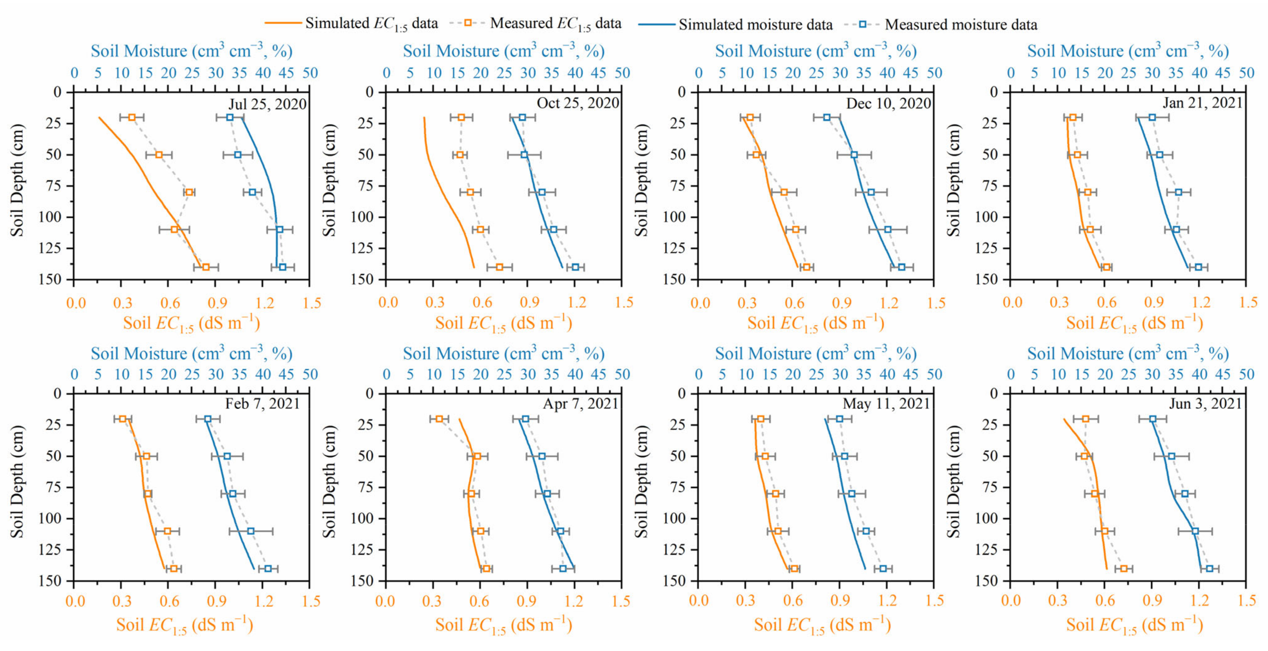
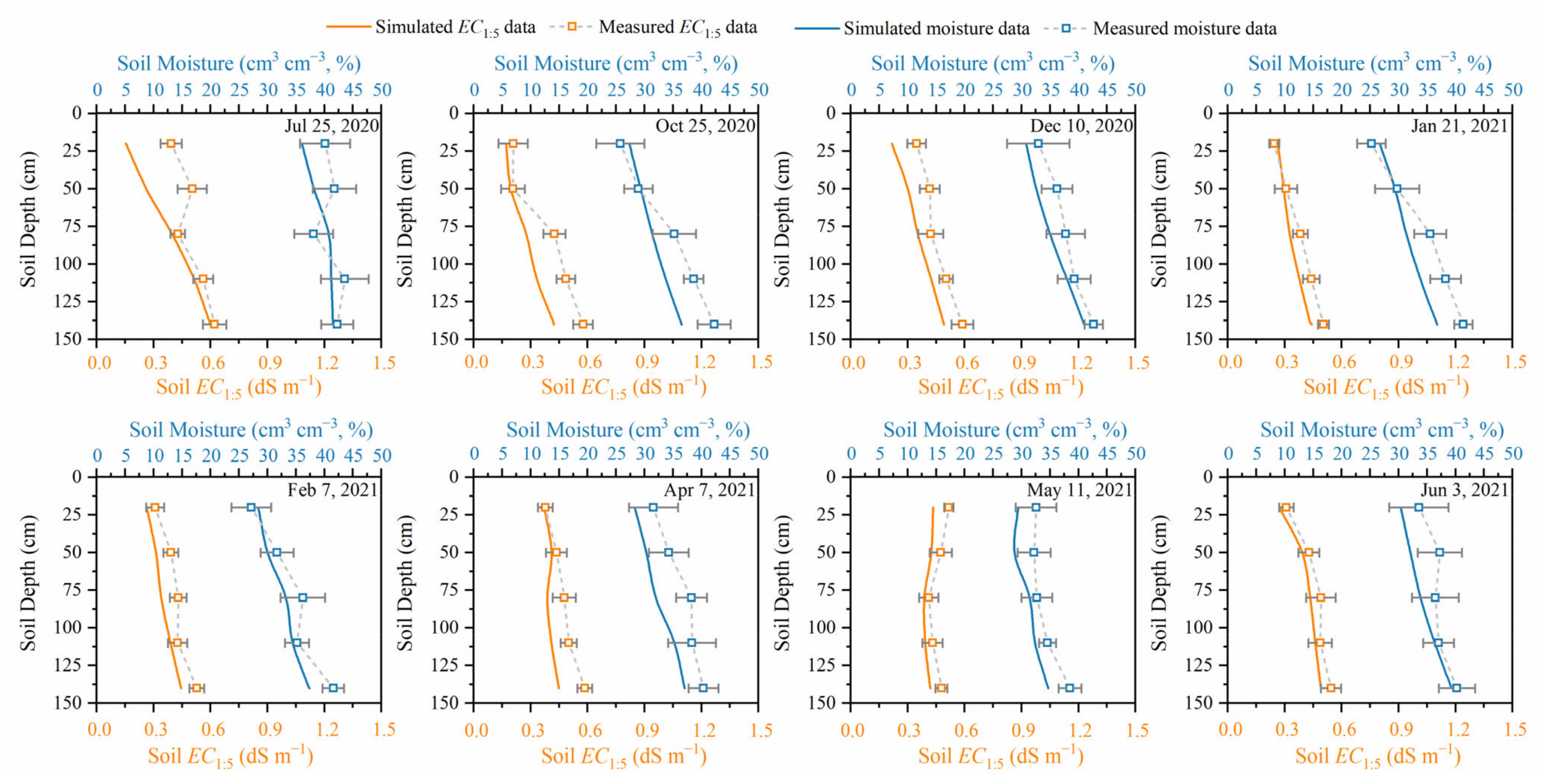
3.1.1. HYDRUS Model Calibration and Validation

The measured moisture and salt contents (EC1:5) in the soil profiles of fields A and B throughout the investigation period were compared with the corresponding simulation values for model calibration (Figure 5) and further validation (Figure 6), respectively. The simulated data at different soil depths and dates adequately represented soil water and salt distribution under SPD, and captured the variation trend of the measured data during the experimental period. The statistical indicators used to evaluate the differences between the measured and simulated values are presented in Table 4. Negative ME values were obtained for both soil moisture and salt content during calibration and validation, indicating a general underestimation during the simulation period. The extent of deviation in moisture content can be attributed to the assumption of constant root distribution characteristics, which likely increased crop water uptake and reduced the moisture content among root zones that involve the field sampling positions. By contrast, the over/underestimated salt content can be partly attributed to the model running at the daily step with the assumption that the rainfall amount is evenly varied daily, which potentially limits the occurrence of surface runoff caused by short-term (hourly or by the minute) heavy rainfall events and converts more rainwater to infiltration for soil leaching. Moreover, the statistical indicators suggest a lower model accuracy for representing soil salt dynamics than soil moisture because higher RMSEn values and lower NSE and R2 values were observed in both the calibration and validation stages. The explanation was that HYDRUS establishes the convection dispersion equation based on the solution of Richards’ equation, and thus the simulation error of soil moisture will be added to the solute simulation. Although the statistical errors in the validation stage were generally larger than those in the calibration stage for both soil moisture and salt content simulations, the corresponding indicators of RMSEn, NSE, and R2 for evaluating the established model performance all ranged within an acceptable limit. Generally, despite certain deviations between the measured and simulated salt contents, the HYDRUS-simulated results showed reasonable agreement among field-measured values, and the estimation errors were on the lower side of the range reported in previous model studies related to subsurface pipe drainage [18,62].

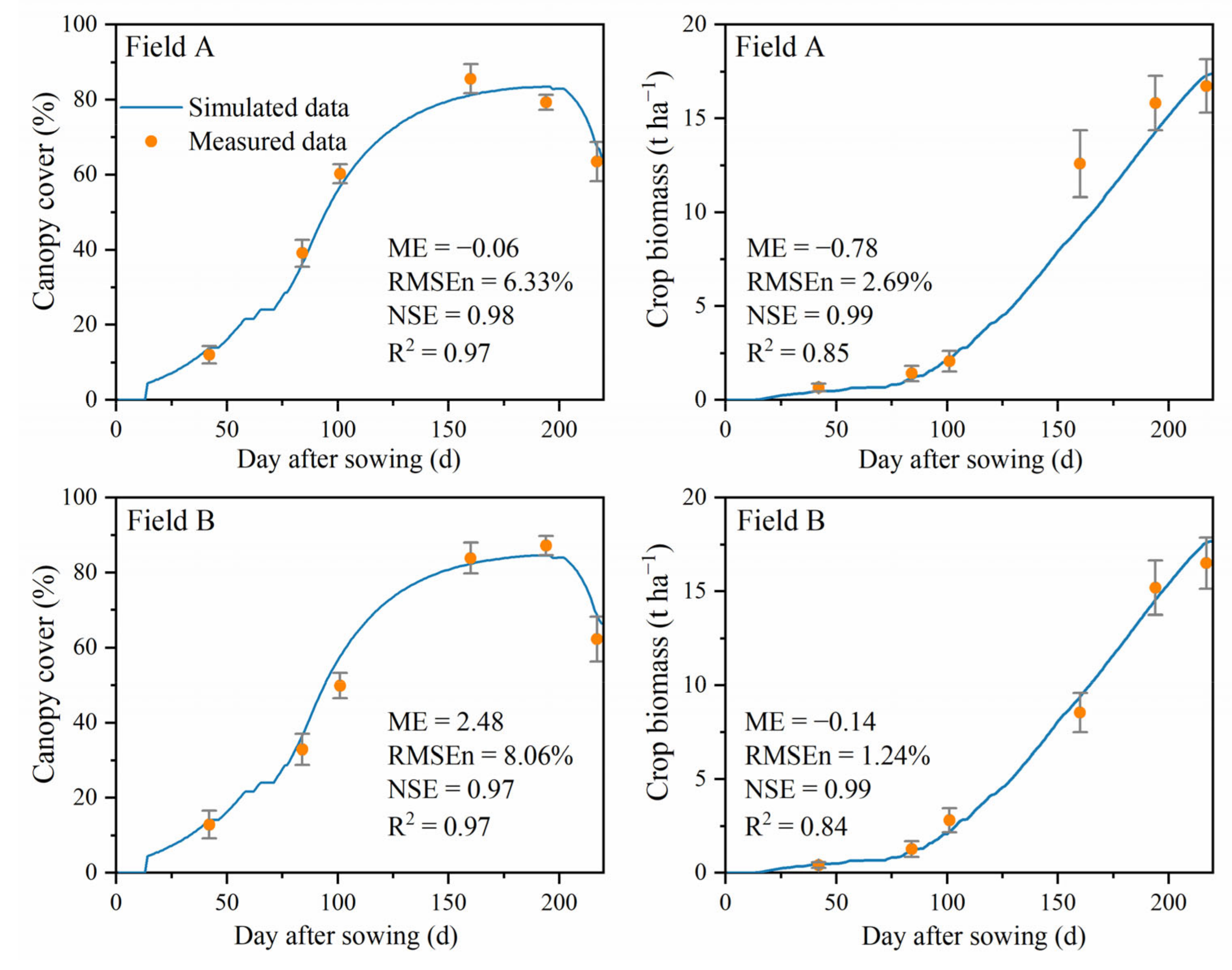
3.1.2. AquaCrop Model Calibration and Validation

Figure 7 presents the difference between the field-measured and AquaCrop-simulated seasonal progression of winter wheat canopy cover and biomass. In the calibration stage, the negative ME values suggested that the AquaCrop model generally underestimated both canopy cover and biomass. The simulated values tended to be lower than the measured values during the middle growth stage of winter wheat. In the validation stage, the AquaCrop model results overestimated the canopy cover, and this tendency was more pronounced before reviving the green stage (approximately 100 DAS), while the biomass progression was slightly underestimated. Notably, the positive deviation of the simulated final biomass values from the corresponding measured values could result from the stable parameter setting of normalized water productivity (15 g m−2) throughout the wheat growing season, because water productivity represents the rate of crop transpiration converted to biomass production, which is expected to decline during the late growth stage [63,64]. Furthermore, the AquaCrop model estimates the flux of groundwater capillary transport to the soil surface based on the total water balance, resulting in the dynamic distributions of soil water being less extensively described [65]. By contrast, the HYDRUS model calculated the upward movement of soil water from the saturated zone of groundwater to the unsaturated zone based on the finite element method in a field-based model flow domain. Therefore, the inconsistent calculation pattern between these two models inevitably aggravates the prediction errors. Overall, despite certain occasional deviations between simulated and measured values of canopy cover and biomass, the corresponding RMSEn was lower than 10%, and NSE and R2 were close to 1 for both calibration and validation stages. These findings indicate that the established model presents a satisfactory simulation accuracy and further proves the feasibility of using the AquaCrop model to evaluate crop growth in SPD-applied fields based on the HYDRUS-estimated water table behaviors.

3.2. Scenario Evaluation and Analysis

3.2.1. Response of Drainage Performance to Groundwater Salinity

In Figure 8, the 30-year variation in solute concentration within the soil layer above the drain depth (0–0.9 m depth) is nearly in conformity with the annual precipitation, with high values of soil solute concentration in dry years and lower values in wet years. The groundwater salinity is the determinant of the range of soil solute concentration, because the average soil solute concentration under low groundwater salinity conditions for scenarios with different drainage spacings were 65.9% and 51.2% lower than those of high and medium salinity scenarios throughout the simulation period. Compared with the no-SPD scenario (ND), the 30-year average values of soil solute concentration of the four drain-spacing scenarios decreased by 11.1%, 13.8%, and 14.6% with groundwater salinity at low, medium, and high levels, respectively. However, there was no continuous downward trend of soil solute concentration during the long-term application of SPD, indicating that the desalination performance of SPD may not be relevant to its application time when rainfall is leached with a constant groundwater salinity. In fact, the average shoreline extension rate was approximately 200 m year−1 during the last half century [66] in the coastal tidal flats of Jiangsu Province, and the salinity level of shallow groundwater generally declines as the distance from the shoreline increases [67]. Therefore, the salt content in the soil profile should gradually decrease during the long-term development of muddy deposition in nearshore areas, and the application of SPD can enhance such decreasing trends to improve the efficiency of land reclamation. Additionally, the discrepancies among the four drainage scenarios increased as the salinity level of the groundwater increased from low to high. For instance, the 30-year average value of the 10 m spacing scenario was only 0.22 g L−1 lower than that of the 40 m spacing scenario under low groundwater salinity conditions, whereas under medium and high salinity levels, the difference between these two scenarios increased to 0.50 and 0.67 g L−1, respectively. This phenomenon suggests that the advantage of SPD with smaller drain spacing in controlling soil solute could be further pronounced as the field salinization is aggravated by increased groundwater salinity.
After applying SPD for 30 years under different groundwater salinity conditions, the total amount of discharged water and solute mass was estimated using the established field-size HYDRUS model, as shown in Figure 9. The cumulative water discharge amount was negatively related to the drain spacing and showed less response to the groundwater salinity. The scenarios with different drain spacings obtained the highest discharge amounts at high salinity levels, possibly due to the salt stress limiting the root water uptake and ensuring relatively high soil moisture [13]. In addition, for all the groundwater salinity levels, the values of the cumulative discharged solute mass of the 40 m spacing scenarios were 74.6%, 47.2%, and 29.3% lower than those of the scenarios with 10 m, 20 m, and 30 m spacing, respectively, suggesting that increased drainage spacing resulted in a reduction in salt discharge, while the extent of such reduction would gradually decrease with further increase in the drain spacing [15].

3.2.2. Response of Crop Yield, Water Productivity, and Groundwater Supply to Different Scenarios

Figure 10 presents the box plots of the AquaCrop-simulated grain yield (GY), water productivity (WP), and groundwater supply (GS) to winter wheat under different precipitation category years and SPD drain spacings. As precipitation is the dominant water source for rain-fed winter wheat growth, the GY and WP values generally varied in an accordant tendency, with higher values in wet years and lower values in dry years, which is in contrast to the variation in GS. Several studies reported similar results that shallow groundwater tends to move upward by capillary forces under deficit irrigation conditions to supply evapotranspiration, but such a supplement may not effectively improve crop production when crops are subject to the restricted water table in drained fields [54,68]. In terms of groundwater salinity, the values of GY, WP, and GS under low groundwater salinity almost varied in the same range in the same precipitation years. In contrast, under the medium and high groundwater salinity, the SPD-applied scenarios generally produced higher GY and WP values compared to the no-SPD scenarios, and the corresponding increases in GY, WP, and GS were 0.81–1.65 t ha−1, 0.13–0.35 kg m−3, and 6.06–31.03 mm, respectively.
Additionally, among the four SPD-applied scenarios, the GY and WP values changed little with the drain spacing, and the maximum differences in GY and WP between the 10 m and 40 m drain spacing were only 0.37 t ha−1 and 0.11 kg m−3, respectively. The GS values slightly decreased with increasing drain spacing in the normal and wet years under medium and high groundwater salinity, the average GS values of 10 m drain spacing scenarios increased by 2.16%, 3.47%, and 3.66% as compared to the 20 m, 30 m, and 40 m drain spacing scenarios, respectively. This is because the closer drain spacing allowed more of the infiltrated water to laterally discharge rather than undergo deep percolation for groundwater recharge [69], resulting in less upward flux of capillary supply for evapotranspiration [70,71].

4. Conclusions

This study demonstrated that the applicability of the AquaCrop model in simulating crop growth in fields with the SPD system could be improved by employing the HYDRUS model-predicted water table behaviors. The HYDRUS and AquaCrop were co-applied to assess the long-term influence of different precipitation years and groundwater salinity on the effect of the SPD systems with different drain spacings on soil water–salt transport, crop yield, water productivity, and groundwater upward supply. Results suggest that narrowing the drain spacing could facilitate soil solute discharge under rainfall leaching and restrict soil salinization caused by capillary-raised saline groundwater. However, there was no continuous downward trend of soil solute concentration during the long-term application of SPD when the drain fields were subjected to constant groundwater salinity. Additionally, the application of SPD could increase grain yield by 0.81–1.65 t ha−1, water productivity by 0.13–0.35 kg m−3, and groundwater supply by 6.06–31.03 mm compared to the no-SPD scenarios, but such increases would be less pronounced in dry years with groundwater salinity at the low level. The present study’s findings indicated that the cooperation of hydrologic and crop models can provide theoretical guidance for long-term agricultural salinity management in coastal areas, where rainwater is regarded as the primary resource for soil leaching and crop water uptake. Additionally, a small drain spacing layout pattern may lead to increased equipment installation and maintenance investment. Therefore, a trade-off between land reclamation performance and infrastructure expenditure of the SPD system should be investigated further.

Author Contributions

Conceptualization, P.L. and Z.J.; methodology, Y.Z.; software, P.L. and Y.Y.; validation, P.L., Z.J. and W.L.; formal analysis, P.L.; investigation, Y.Y. and W.L.; resources, P.L. and Y.Z.; data curation, P.L.; writing—original draft preparation, P.L. and Z.J.; writing—review and editing, P.L. and Z.J.; visualization, P.L. and Y.Y.; supervision, W.L.; project administration, P.L.; funding acquisition, P.L. and Z.J. All authors have read and agreed to the published version of the manuscript.

Funding

This research was funded by the National Natural Science Foundation of China, grant number 52109068; the China Postdoctoral Science Foundation, grant number 2022M712690; the Science and Technology Funding project of City-School Cooperation in Yangzhou, China, grant number YZU202101; the Postdoctoral Research Funding Program of Jiangsu province, China, grant number 2021K220B.

Data Availability Statement

The data that support this study cannot be publicly shared due to ethical or privacy reasons and may be shared upon reasonable request to the corresponding author if appropriate.

Acknowledgments

We are grateful to the editors and reviewers for their valuable suggestions on improving the manuscript.

Conflicts of Interest

The authors declare no conflict of interest.

References

  1. Schuerch, M.; Spencer, T.; Temmerman, S.; Kirwan, M.L.; Wolff, C.; Lincke, D.; McOwen, C.J.; Pickering, M.D.; Reef, R.; Vafeidis, A.T.; et al. Future response of global coastal wetlands to sea-level rise. Nature 2018, 561, 231–234. [Google Scholar] [CrossRef] [Green Version]
  2. Wu, W.T.; Yang, Z.Q.; Tian, B.; Huang, Y.; Zhou, Y.X.; Zhang, T. Impacts of coastal reclamation on wetlands: Loss, resilience, and sustainable management. Estuar. Coast. Shelf Sci. 2018, 210, 153–161. [Google Scholar] [CrossRef]
  3. Robinson, C.E.; Xin, P.; Santos, I.R.; Charette, M.A.; Li, L.; Barry, D.A. Groundwater dynamics in subterranean estuaries of coastal unconfined aquifers: Controls on submarine groundwater discharge and chemical inputs to the ocean. Adv. Water Resour. 2018, 115, 315–331. [Google Scholar] [CrossRef]
  4. Zhan, L.C.; Xin, P.; Chen, J.S. Subsurface salinity distribution and evolution in low-permeability coastal areas after land reclamation: Field investigation. J. Hydrol. 2022, 612, 128250. [Google Scholar] [CrossRef]
  5. Long, X.H.; Liu, L.P.; Shao, T.Y.; Shao, H.B.; Liu, Z.P. Developing and sustainably utilize the coastal mudflat areas in China. Sci. Total Environ. 2016, 569, 1077–1086. [Google Scholar] [CrossRef]
  6. Iost, S.; Landgraf, D.; Makeschin, F. Chemical soil properties of reclaimed marsh soil from Zhejiang Province PR China. Geoderma 2007, 142, 245–250. [Google Scholar] [CrossRef]
  7. Velmurugan, A.; Swarnam, T.P.; Lal, R. Effect of land shaping on soil properties and crop yield in tsunami inundated coastal soils of Southern Andaman Island. Agric. Ecosyst. Environ. 2015, 206, 1–9. [Google Scholar] [CrossRef]
  8. Setiawan, I.; Morgan, L.; Doscher, C.; Ng, K.; Bosserelle, A. Mapping shallow groundwater salinity in a coastal urban setting to assess exposure of municipal assets. J. Hydrol. Reg. Stud. 2022, 40, 100999. [Google Scholar] [CrossRef]
  9. Forkutsa, I.; Sommer, R.; Shirokova, Y.I.; Lamers, J.P.A.; Kienzler, K.; Tischbein, B.; Martius, C.; Vlek, P.L.G. Modeling irrigated cotton with shallow groundwater in the Aral Sea Basin of Uzbekistan: I. Water dynamics. Irrig. Sci. 2009, 27, 331–346. [Google Scholar] [CrossRef]
  10. Islam, M.N.; Bell, R.W.; Barrett-Lennard, E.G.; Maniruzzaman, M.J.A.f.S.D. Shallow surface and subsurface drains alleviate waterlogging and salinity in a clay-textured soil and improve the yield of sunflower in the Ganges Delta. Agron. Sustain. Dev. 2022, 42, 16. [Google Scholar] [CrossRef]
  11. Fang, D.; Guo, K.; Ameen, A.; Wang, S.C.; Xie, J.; Liu, J.T.; Han, L.P. A Root Density Tradeoff in an Okra-Assisted Subsurface Pipe Drainage System for Amelioration of Saline Soil. Agronomy 2022, 12, 866. [Google Scholar] [CrossRef]
  12. Sloan, B.P.; Basu, N.B.; Mantilla, R. Hydrologic impacts of subsurface drainage at the field scale: Climate, landscape and anthropogenic controls. Agric. Water Manag. 2016, 165, 1–10. [Google Scholar] [CrossRef]
  13. Wang, Z.H.; Heng, T.; Li, W.H.; Zhang, J.Z.; Zhangzhong, L.L. Effects of subsurface pipe drainage on soil salinity in saline-sodic soil under mulched drip irrigation. Irrig. Drain. 2020, 69, 95–106. [Google Scholar] [CrossRef]
  14. Nozari, H.; Azadi, S.; Zali, A. Experimental study of the temporal variation of drain water salinity at different drain depths and spacing in the presence of saline groundwater. Sustain. Water Resour. Manag. 2018, 4, 887–895. [Google Scholar] [CrossRef]
  15. Shao, X.H.; Chang, T.T.; Cai, F.; Wang, Z.Y.; Huang, M.Y. Effects of subsurface drainage design on soil desalination in coastal resort of China. J. Food Agric. Environ. 2012, 10, 935–938. [Google Scholar]
  16. Tuohy, P.; O’Loughlin, J.; Fenton, O. Modeling performance of a tile drainage system incorporating mole drainage. Trans. Asabe 2018, 61, 169–178. [Google Scholar] [CrossRef] [Green Version]
  17. Bonaiti, G.; Borin, M. Efficiency of controlled drainage and subirrigation in reducing nitrogen losses from agricultural fields. Agric. Water Manag. 2010, 98, 343–352. [Google Scholar] [CrossRef]
  18. Ebrahimian, H.; Noory, H. Modeling paddy field subsurface drainage using HYDRUS-2D. Paddy Water Environ. 2015, 13, 477–485. [Google Scholar] [CrossRef]
  19. Lu, P.R.; Zhang, Z.Y.; Sheng, Z.; Huang, M.Y.; Zhang, Z.M. Assess Effectiveness of Salt Removal by a Subsurface Drainage with Bundled Crop Straws in Coastal Saline Soil Using HYDRUS-3D. Water 2019, 11, 943. [Google Scholar] [CrossRef] [Green Version]
  20. Tao, Y.; Li, N.; Wang, S.L.; Chen, H.R.; Guan, X.Y.; Ji, M.Z. Simulation study on performance of nitrogen loss of an improved subsurface drainage system for one-time drainage using HYDRUS-2D. Agric. Water Manag. 2021, 246, 106698. [Google Scholar] [CrossRef]
  21. Krevh, V.; Filipovic, V.; Filipovic, L.; Matekovic, V.; Petosic, D.; Mustac, I.; Ondrasek, G.; Bogunovic, I.; Kovac, Z.; Pereira, P.; et al. Modeling seasonal soil moisture dynamics in gley soils in relation to groundwater table oscillations in eastern Croatia. Catena 2022, 211, 105987. [Google Scholar] [CrossRef]
  22. Feddes, R.A. Simulation of field water use and crop yield. Soil Sci. 1978, 129, 193. [Google Scholar]
  23. Simunek, J.; Hopmans, J.W. Modeling compensated root water and nutrient uptake. Ecol. Model. 2009, 220, 505–521. [Google Scholar] [CrossRef]
  24. Ranjbar, A.; Rahimikhoob, A.; Ebrahimian, H.; Varavipour, M. Simulation of nitrogen uptake and dry matter for estimation of nitrogen nutrition index during the maize growth period. J. Plant Nutr. 2022, 45, 920–936. [Google Scholar] [CrossRef]
  25. Zhou, J.; Cheng, G.D.; Li, X.; Hu, B.X.; Wang, G.X. Numerical Modeling of Wheat Irrigation using Coupled HYDRUS and WOFOST Models. Soil Sci. Soc. Am. J. 2012, 76, 648–662. [Google Scholar] [CrossRef]
  26. Roy, P.C.; Guber, A.; Abouali, M.; Nejadhashemi, A.P.; Deb, K.; Smucker, A.J.M. Crop yield simulation optimization using precision irrigation and subsurface water retention technology. Environ. Model. Softw. 2019, 119, 433–444. [Google Scholar] [CrossRef]
  27. Zhao, J.; Han, T.; Wang, C.; Jia, H.; Worqlul, A.W.; Norelli, N.; Zeng, Z.H.; Chu, Q.Q. Optimizing irrigation strategies to synchronously improve the yield and water productivity of winter wheat under interannual precipitation variability in the North China Plain. Agric. Water Manag. 2020, 240, 106298. [Google Scholar] [CrossRef]
  28. Goosheh, M.; Pazira, E.; Gholami, A.; Andarzian, B.; Panahpour, E. Improving Irrigation Scheduling of Wheat to Increase Water Productivity in Shallow Groundwater Conditions Using Aquacrop. Irrig. Drain. 2018, 67, 738–754. [Google Scholar] [CrossRef]
  29. Zhang, C.; Xie, Z.A.; Wang, Q.J.; Tang, M.; Feng, S.Y.; Cai, H.J. AquaCrop modeling to explore optimal irrigation of winter wheat for improving grain yield and water productivity. Agric. Water Manag. 2022, 266, 107580. [Google Scholar] [CrossRef]
  30. Hammami, Z.; Qureshi, A.S.; Sahli, A.; Gauffreteau, A.; Chamekh, Z.; Ben Azaiez, F.E.; Ayadi, S.; Trifa, Y. Modeling the Effects of Irrigation Water Salinity on Growth, Yield and Water Productivity of Barley in Three Contrasted Environments. Agronomy 2020, 10, 1459. [Google Scholar] [CrossRef]
  31. Hsiao, T.C.; Heng, L.; Steduto, P.; Rojas-Lara, B.; Raes, D.; Fereres, E. AquaCrop-The FAO Crop Model to Simulate Yield Response to Water: III. Parameterization and Testing for Maize. Agron. J. 2009, 101, 448–459. [Google Scholar] [CrossRef]
  32. Akhtar, F.; Tischbein, B.; Awan, U.K. Optimizing Deficit Irrigation Scheduling Under Shallow Groundwater Conditions in Lower Reaches of Amu Darya River Basin. Water Resour. Manag. 2013, 27, 3165–3178. [Google Scholar] [CrossRef]
  33. Tenreiro, T.R.; Jerabek, J.; Gomez, J.A.; Zumr, D.; Martinez, G.; Garcia-Vila, M.; Fereres, E. Simulating water lateral inflow and its contribution to spatial variations of rainfed wheat yields. Eur. J. Agron. 2022, 137, 126515. [Google Scholar] [CrossRef]
  34. Shirokova, Y.; Forkutsa, I.; Sharafutdinova, N. Use of Electrical Conductivity Instead of Soluble Salts for Soil Salinity Monitoring in Central Asia. Irrig. Drain. Syst. 2000, 14, 199–205. [Google Scholar] [CrossRef]
  35. Patrignani, A.; Ochsner, T.E. Canopeo: A Powerful New Tool for Measuring Fractional Green Canopy Cover. Agron. J. 2015, 107, 2312–2320. [Google Scholar] [CrossRef] [Green Version]
  36. Razzaghi, F.; Zhou, Z.J.; Andersen, M.N.; Plauborg, F. Simulation of potato yield in temperate condition by the AquaCrop model. Agric. Water Manag. 2017, 191, 113–123. [Google Scholar] [CrossRef]
  37. Abbasi, F.; Simunek, J.; Feyen, J.; van Genuchten, M.T.; Shouse, P.J. Simultaneous inverse estimation of soil hydraulic and solute transport parameters from transient field experiments: Homogeneous soil. Trans. ASAE 2003, 46, 1085–1095. [Google Scholar] [CrossRef] [Green Version]
  38. Mualem, Y. A new model for predicting the hydraulic conductivity of unsaturated porous media. Water Resour. Res. 1976, 12, 513–522. [Google Scholar] [CrossRef] [Green Version]
  39. Genuchten, M.T.v. A Closed-form Equation for Predicting the Hydraulic Conductivity of Unsaturated Soils. Soil Sci. Soc. Am. J. 1980, 44, 892–898. [Google Scholar] [CrossRef] [Green Version]
  40. Allen, R.G.; Pereira, L.S.; Raes, D.; Smith, M. Crop Evapotranspiration—Guidelines for Computing Crop Water Requirements; Food and Agriculture Organization of the United Nations (FAO): Rome, Italy, 1998. [Google Scholar]
  41. Zhu, Y.H.; Ren, L.L.; Horton, R.; Lu, H.S.; Wang, Z.L.; Yuan, F. Estimating the Contribution of Groundwater to the Root Zone of Winter Wheat Using Root Density Distribution Functions. Vadose Zone J. 2018, 17, 1–15. [Google Scholar] [CrossRef] [Green Version]
  42. Nielsen, D.C.; Miceli-Garcia, J.J.; Lyon, D.J. Canopy Cover and Leaf Area Index Relationships for Wheat, Triticale, and Corn. Agron. J. 2012, 104, 1569–1573. [Google Scholar] [CrossRef] [Green Version]
  43. Vrugt, J.A.; van Wijk, M.T.; Hopmans, J.W.; Simunek, J. One-, two-, and three-dimensional root water uptake functions for transient modeling. Water Resour. Res. 2001, 37, 2457–2470. [Google Scholar] [CrossRef] [Green Version]
  44. Schaap, M.G.; Leij, F.J.; van Genuchten, M.T. ROSETTA: A computer program for estimating soil hydraulic parameters with hierarchical pedotransfer functions. J. Hydrol. 2001, 251, 163–176. [Google Scholar] [CrossRef]
  45. Ramos, T.B.; Simunek, J.; Goncalves, M.C.; Martins, J.C.; Prazeres, A.; Pereira, L.S. Two-dimensional modeling of water and nitrogen fate from sweet sorghum irrigated with fresh and blended saline waters. Agric. Water Manag. 2012, 111, 87–104. [Google Scholar] [CrossRef]
  46. Radcliffe, D.E.; Šimůnek, J. Soil Physics with HYDRUS; CRC Press: Boca Raton, FL, USA; Taylor &Francis Group: Abingdon, UK, 2010. [Google Scholar]
  47. Skaggs, T.H.; Shouse, P.J.; Poss, J.A. Irrigating forage crops with saline waters: 2. Modeling root uptake and drainage. Vadose Zone J. 2006, 5, 824–837. [Google Scholar] [CrossRef]
  48. Karandish, F.; Simunek, J. An application of the water footprint assessment to optimize production of crops irrigated with saline water: A scenario assessment with HYDRUS. Agric. Water Manag. 2018, 208, 67–82. [Google Scholar] [CrossRef] [Green Version]
  49. Grattan, S. Irrigation Water Salinity and Crop Production; UCANR Publications: Oakland, CA, USA, 2002; Volume 9. [Google Scholar]
  50. Mondal, M.S.; Saleh, A.F.M.; Akanda, M.A.R.; Biswas, S.K.; Moslehuddin, A.Z.M.; Zaman, S.; Lazar, A.N.; Clarke, D. Simulating yield response of rice to salinity stress with the AquaCrop model. Environ. Sci. -Process. Impacts 2015, 17, 1118–1126. [Google Scholar] [CrossRef] [Green Version]
  51. Foster, T.; Brozovic, N.; Butler, A.P.; Neale, C.M.U.; Raes, D.; Steduto, P.; Fereres, E.; Hsiao, T.C. AquaCrop-OS: An open source version of FAO’s crop water productivity model. Agric. Water Manag. 2017, 181, 18–22. [Google Scholar] [CrossRef]
  52. Saab, M.T.A.; Todorovic, M.; Albrizio, R. Comparing Aqua Crop and CropSyst models in simulating barley growth and yield under different water and nitrogen regimes. Does calibration year influence the performance of crop growth models? Agric. Water Manag. 2015, 147, 21–33. [Google Scholar] [CrossRef]
  53. Raes, D.; Steduto, P.; Hsiao, T.C.; Fereres, E. AquaCrop-The FAO Crop Model to Simulate Yield Response to Water: II. Main Algorithms and Software Description. Agron. J. 2009, 101, 438–447. [Google Scholar] [CrossRef] [Green Version]
  54. Pourgholam-Amiji, M.; Liaghat, A.; Ghameshlou, A.N.; Khoshravesh, M. The evaluation of DRAINMOD-S and AquaCrop models for simulating the salt concentration in soil profiles in areas with a saline and shallow water table. J. Hydrol. 2021, 598, 126259. [Google Scholar] [CrossRef]
  55. Davarpanah, R.; Ahmadi, S.H. Modeling the effects of irrigation management scenarios on winter wheat yield and water use indicators in response to climate variations and water delivery systems. J. Hydrol. 2021, 598, 126269. [Google Scholar] [CrossRef]
  56. Montoya, F.; Camargo, D.; Ortega, J.F.; Corcoles, J.I.; Dominguez, A. Evaluation of Aquacrop model for a potato crop under different irrigation conditions. Agric. Water Manag. 2016, 164, 267–280. [Google Scholar] [CrossRef]
  57. Kumar, M.; Sarangi, A.; Singh, D.K.; Rao, A.R. Modelling the Grain Yield of Wheat in Irrigated Saline Environment with Foliar Potassium Fertilization. Agric. Res. 2018, 7, 321–337. [Google Scholar] [CrossRef]
  58. Xu, J.Z.; Bai, W.H.; Li, Y.W.; Wang, H.Y.; Yang, S.H.; Wei, Z. Modeling rice development and field water balance using AquaCrop model under drying-wetting cycle condition in eastern China. Agric. Water Manag. 2019, 213, 289–297. [Google Scholar] [CrossRef]
  59. Qian, Y.Z.; Zhu, Y.; Ye, M.; Huang, J.S.; Wu, J.W. Experiment and numerical simulation for designing layout parameters of subsurface drainage pipes in arid agricultural areas. Agric. Water Manag. 2021, 243, 106455. [Google Scholar] [CrossRef]
  60. Tao, Y.; Wang, S.L.; Xu, D.; Guan, X.Y.; Ji, M.Z.; Liu, J. Theoretical analysis and experimental verification of the improved subsurface drainage discharge with ponded water. Agric. Water Manag. 2019, 213, 546–553. [Google Scholar] [CrossRef]
  61. Chow, V.T.; Maidment, D.R.; Mays, L.W. Handbook of Applied Hydrology; McGraw-Hill: New York, NY, USA, 1988. [Google Scholar]
  62. Liu, Y.; Ao, C.; Zeng, W.; Kumar Srivastava, A.; Gaiser, T.; Wu, J.; Huang, J. Simulating water and salt transport in subsurface pipe drainage systems with HYDRUS-2D. J. Hydrol. 2021, 592, 125823. [Google Scholar] [CrossRef]
  63. Sandhu, R.; Irmak, S. Assessment of AquaCrop model in simulating maize canopy cover, soil-water, evapotranspiration, yield, and water productivity for different planting dates and densities under irrigated and rainfed conditions. Agric. Water Manag. 2019, 224, 105753. [Google Scholar] [CrossRef]
  64. Huang, M.; Wang, C.; Qi, W.; Zhang, Z.; Xu, H. Modelling the integrated strategies of deficit irrigation, nitrogen fertilization, and biochar addition for winter wheat by AquaCrop based on a two-year field study. Field Crops Res. 2022, 282, 108510. [Google Scholar] [CrossRef]
  65. Raes, D.; Steduto, P.; Hsiao, T.C.; Fereres, E. Reference Manual AquaCrop; FAO Land and Water Division: Rome, Italy, 2012. [Google Scholar]
  66. Song, Y.; Shen, Y.M.; Xie, R.F.; Li, J.L. A DSAS-based study of central shoreline change in Jiangsu over 45 years. Anthr. Coasts 2021, 4, 115–128. [Google Scholar] [CrossRef]
  67. Shang, T.X.; Xu, Z.W.; Gong, X.L.; Li, X.Q.; Tian, S.B.; Guan, Y.X. Application of electrical sounding to determine the spatial distribution of groundwater quality in the coastal area of Jiangsu Province, China. J. Hydrol. 2021, 599, 126348. [Google Scholar] [CrossRef]
  68. Zhang, K.; Shao, G.C.; Wang, Z.Y.; Cui, J.T.; Lu, J.; Gao, Y. Modeling the impacts of groundwater depth and biochar addition on tomato production under climate change using RZWQM2. Sci. Hortic. 2022, 302, 111147. [Google Scholar] [CrossRef]
  69. Aissa, I.B.; Bouarfa, S.; Vincent, B.; Chaumont, C.; Perrier, A. Drainage performance assessment in a modernized oasis system. Irrig. Drain. 2013, 62, 221–228. [Google Scholar] [CrossRef]
  70. Gao, X.Y.; Bai, Y.N.; Huo, Z.L.; Xu, X.; Huang, G.H.; Xia, Y.H.; Steenhuis, T.S. Deficit irrigation enhances contribution of shallow groundwater to crop water consumption in arid area. Agric. Water Manag. 2017, 185, 116–125. [Google Scholar] [CrossRef]
  71. Li, H.J.; Yi, J.; Zhang, J.G.; Zhao, Y.; Si, B.C.; Hill, R.L.; Cui, L.L.; Liu, X.Y. Modeling of Soil Water and Salt Dynamics and Its Effects on Root Water Uptake in Heihe Arid Wetland, Gansu, China. Water 2015, 7, 2382–2401. [Google Scholar] [CrossRef] [Green Version]
Figure 1. Location of the experimental site. Digital Elevation Model data source: National Earth System Science Data Centre, National science & Technology Infrastructure of China (http://www.geodata.cn (accessed on 11 December 2022)).
Agronomy 13 00588 g001
Figure 2. (a) Daily reference crop evapotranspiration (ET0) and precipitation during the investigation. (b) Daily potential evaporation (Ep), transpiration (Tp), and crop coefficient (Kc) during the winter growing season. DAS refers to the days after wheat sowing.
Agronomy 13 00588 g002
Figure 3. Two-dimensional modelling domain of Field B (part of the left side), including imposed boundary conditions and distribution of soil layers.
Agronomy 13 00588 g003
Figure 4. Variation in precipitation and reference evapotranspiration during winter wheat growing season in Dongtai County from 1990 to 2020.
Agronomy 13 00588 g004
Figure 5. Comparison of field-measured and HYDRUS-simulated values of soil moisture and salinity (EC1:5) in field A during the investigation period for model calibration. Note: The date and its corresponding stage are before sowing (25 July and 25 October 2020), overwintering stage (10 December 2020 and 21 January 2021), reviving green stage (7 February 2021), jointing stage (7 April 2021), grain-filling stage (11 May 2021), and maturity stage (3 June 2021). The error bars refer to the standard error of replicates as follows.
Agronomy 13 00588 g005
Figure 6. Comparison of field-measured and HYDRUS-simulated values of soil moisture and salinity (EC1:5) in field B during the investigation period for model validation.
Agronomy 13 00588 g006
Figure 7. Comparison of field-measured and AquaCrop-simulated values of canopy cover and biomass during the winter wheat growth season for model calibration (Field A) and validation (Field B).
Agronomy 13 00588 g007
Figure 8. Temporal dynamics of soil solute concentrations at 0–0.9 m soil depth under low (a), medium (b), and high (c) groundwater salinity levels and five drain spacings in 30 years’ meteorological condition (1990–2020). ND refers to the no-SPD scenario.
Agronomy 13 00588 g008
Figure 9. Simulation of 30 years cumulative discharge of water (point line) and solute mass (bar chart) by subsurface pipe drainage under low, medium, and high groundwater salinity condition.
Agronomy 13 00588 g009
Figure 10. Comparison of simulated (a) grain yield, (b) water productivity, and (c) groundwater supply in a rain-fed winter wheat field under different groundwater salinity levels and drain spacings in wet, normal, and dry years. The top and bottom range of the box represent percentiles 25 and 75 of data. The box whisker represents an outlier range. The lines and red squares within the box represent median and mean values, respectively.
Agronomy 13 00588 g010
Table 1. Soil properties in the experimental site.
Depth (cm)Bulk Density (g cm−3)Field Capacity (cm3 cm−3)Wilting Point (cm−3 cm−3)Saturated Water Content (cm−3 cm−3)Mechanical Composition (%)Soil Texture
SandSlitClay
0–301.36 a0.22 a0.12 a0.46 b40.956.32.8Silt loam
30–1001.42 b0.29 b0.14 a0.42 a35.461.33.3
100–2001.44 b0.31 b0.15 a0.42 a35.560.44.1
200–3001.45 b0.32 b0.15 a0.41 a33.962.23.9
Note: Data are means of five replications, and those followed without the same letter differ significantly at p = 0.05 level. Soil textures are determined by the USDA (United States Department of Agriculture) textural soil classification system.
Table 2. van Genuchtens parameters describing soil hydraulic properties used in this model study.
Soil Layer (cm)θr (cm3 cm−3)θs (cm3 cm−3)αnlKs (cm day−1)
0~30 cm0.0370.4630.0191.4190.5105.31
30~300 cm0.0410.4150.0131.4530.558.52
NOTE: θr and θs denote the residual and saturated water contents; α is the inverse of the air-entry value; n is a pore size distribution index; l is a pore connectivity parameter, set to 0.5 as proved valid for most soil types [38]; and Ks is the saturated hydraulic conductivity.
Table 3. Input parameters of AquaCrop model used in this study.
Parameter DescriptionValueStatus
Non-conservative parameters
    Sowing rate250 kg seed hm−2M
    Cover per seeding1.5 cm2 plant M
    Initial canopy cover5.2%M
    Canopy growth coefficient3.2% day−1C
    Canopy decline coefficient6.9% day−1C
    Maximum canopy cover93%C
    Time from sowing to emergence12 dayM
    Time from sowing to max canopy175 dayM
    Time from sowing to senescence 197 dayM
    Time from sowing to maturity 219 dayM
    Time from sowing to flowing 181 dayM
    Minimum effective rooting depth0.3 mC
    Maximum effective rooting depth1.15C
    Time from sowing to maximum rooting depth90 dayC
    Sharp factor describing root zone expansion1.5D
    Reference harvest index41%C
    Minimum temperature of pollination fail5 °CD
    Maximum temperature of pollination fail35 °CD
    Salinity stress, lower thresholds 6 dS m−1D
    Salinity stress, upper thresholds20 dS m−1D
Conservative parameters
    Base temperature0 °CD
    Upper temperature26 °CD
    Canopy cover per seeding1.5 cm2 Plant−1D
    Normalized crop water productivity15 g m−2D
    Canopy expansion, upper threshold0.2%D
    Canopy expansion, lower threshold0.65%D
    Stomatal conductance threshold0.65%D
    Stomata stress coefficient curve shape2.5D
    Senescence stress upper threshold0.7%D
  Senescence stress coefficient curve shape2.5D
Note: Status M means the value of the parameter refers to the field measurement; Status D means the value of the parameter is taken from the model reference manual; Status C means the value was obtained by model calibration.
Table 4. Statistical evaluation of HYDRUS models for simulating soil moisture and salt content.
StageData SeriesMERMSEnNSER2
CalibrationMoisture (cm3 cm−3)−1.6117.72%0.7490.822
Salt content (dS m−1)−0.05818.63%0.6770.764
ValidationMoisture (cm3 cm−3)−3.45211.71%0.5950.778
Salt content (dS m−1)−0.09829.30%0.4340.690
Disclaimer/Publisher’s Note: The statements, opinions and data contained in all publications are solely those of the individual author(s) and contributor(s) and not of MDPI and/or the editor(s). MDPI and/or the editor(s) disclaim responsibility for any injury to people or property resulting from any ideas, methods, instructions or products referred to in the content.

