A Comprehensive Step-by-Step Guide to Using Data Science Tools in the Gestion of Epidemiological and Climatological Data in Rice Production Systems

Abstract

The application of data science (DS) techniques has become increasingly essential in various fields, including epidemiology and climatology in agricultural production systems. In this sector, traditionally large amounts of data are acquired, but not well-managed and -analyzed as a basis for evidence-based decision-making processes. Here, we present a comprehensive step-by-step guide that explores the use of DS in managing epidemiological and climatological data within rice production systems under tropical conditions. Our work focuses on using the multi-temporal dataset associated with the monitoring of diseases and climate variables in rice in Colombia during eight years (2012–2019). The study comprises four main phases: (I) data cleaning and organization to ensure the integrity and consistency of the dataset; (II) data management involving web-scraping techniques to acquire climate information from free databases, like WordClim and Chelsa, validation against in situ weather stations, and bias removal to enrich the dataset; (III) data visualization techniques to effectively represent the gathered information, and (IV) a basic analysis related to the clustering and climatic characterization of rice-producing areas in Colombia. In our work, a process of evaluation and the validation of climate data are conducted based on errors (r, R^2, MAE, RSME) and bias evaluation metrics. In addition, in phase II, climate clustering was conducted based on a PCA and K-means algorithm. Understanding the association of climatic and epidemiological data is pivotal in predicting and mitigating disease outbreaks in rice production areas. Our research underscores the significance of DS in managing epidemiological and climatological data for rice production systems. By applying a protocol responsible for DS tools, our study provides a solid foundation for further research into disease dynamics and climate interactions in rice-producing regions and other crops, ultimately contributing to more informed decision-making processes in agriculture.

1. Introduction

Rice (Oryza sativa L.) is a cereal of high importance for humans, given that it is produced on almost all continents and is a staple food in the diets of more than half of the world’s population [1]. According to the FAO, world production in 2018 was 761 million tons (t), with a cultivation area of 164 million hectares (ha) [2]. In Colombia, the rice cultivation area in 2020 was 596,414 ha, making up approximately 35% of the total area planted in semi-annual cycle crops [3] Rice cultivation occurs in 23 departments and 211 municipalities in Colombia, involving more than 16,000 producers and 25,000 agricultural production units (APUs) [4]. Health problems of biotic origin, caused by emerging and re-emerging pests and diseases, are a significant problem in rice production, and generate losses of more than 25% of the global production, with losses of between 80 and 100% in severe cases [5,6].

The behavior of pathogens and the diseases they cause in plants are dynamic in nature, and their importance varies depending on multiple factors, such as variation in environmental conditions, the genetic component of the host, the intensity of the production system, and changes in the genetic and pathogenic variabilities of the pathogen [7]. In the rice production systems across the world, it has been identified under different data analysis approaches that diseases are affected by meteorological variables, and this information has been used to predict their behavior in space and time [8,9].

Given that the space–time dynamics of diseases and their potential impact on production systems are highly influenced by edaphoclimatic variables, it is necessary to guarantee a level of confidence in the meteorological data, since the representativeness and quality of this can considerably influence the accuracy, precision, and reproducibility of the models [9,10]. However, guaranteeing the availability, timeliness, quality, and representativeness of the meteorological data in the spatial and temporal dimensions required according to the scale of analysis is a significant challenge. In this regard, the most reliable sources of meteorological data are those from in situ observations from conventional or automatic stations that comply with the guidelines of the WMO (World Meteorological Organization). However, these observations are expensive and, in many cases, unviable, given the high climatic variability. A solution to this is to evaluate, validate, and eliminate the bias of synthetic climate products derived from remote sensors, re-analysis, weather radars, and other tools [11,12].

These tools include previously validated global, spatialized, and freely accessible databases, such as CHELSA and Worldclim (WC), which can solve some of the limitations of obtaining the meteorological data described above. The CHELSA database originates from downscaling the ERA-Interim climate reanalysis to a 1 km resolution [13,14]. Meanwhile, WC corresponds to a set of average monthly interpolated climate data from meteorological stations on a multi-resolution grid [15]. These datasets have been validated and used in studies for purposes of flow estimation, evapotranspiration, the estimation of precipitation and its spatio-temporal variability, and for modeling the distribution of pathogen populations in plants as a function of climate [16,17,18,19].

The implementation of epidemiological simulation models that use climatic or agrometeorological variables as predictors is based on the free and open access to meteorological data at local and regional levels. However, the data volume required for a high-resolution representation of the Earth’s surface of approximately 30–33 arcseconds (900 m to 1 km) [20] requires intelligent data reductions and reference point prioritization; therefore, high-level skills and advanced computing are needed to execute, analyze, and adjust the models if necessary [21,22].

For this reason, data science (DS) is a useful alternative to classical analysis methods, given its ability to analyze a large volume (size) and variety (complex data sources and structure) of data; to assess its veracity (uncertain quality) and value; as well as its speed (fast-rate acquisition rate) [23,24]. DS is an interdisciplinary field focusing on the study of methods and techniques to extract knowledge from data and help us understand multiple phenomena [25]. The process of applying DS concepts is divided into four stages: (i) data acquisition, (ii) data cleaning, (iii) visualization, and (iv) analysis [26].

Considering the abovementioned points, in this work, a robust methodological process based on DS and the spatial analysis of data of climatic and epidemiological origins in productive systems of commercial rice cultivation in Colombia is proposed as a basis for the design and management of databases, their visualization, and the application of analysis tools. The purpose of these tools is to find spatio-temporal patterns that favor decision-making behavior in agricultural planning and the selection of techniques and technologies, as well as climate-smart agricultural practices for rice production. As such, this work aims to apply DS tools to the management of climatic and epidemiological information in rice production systems in Colombia.

2. Materials and Methods

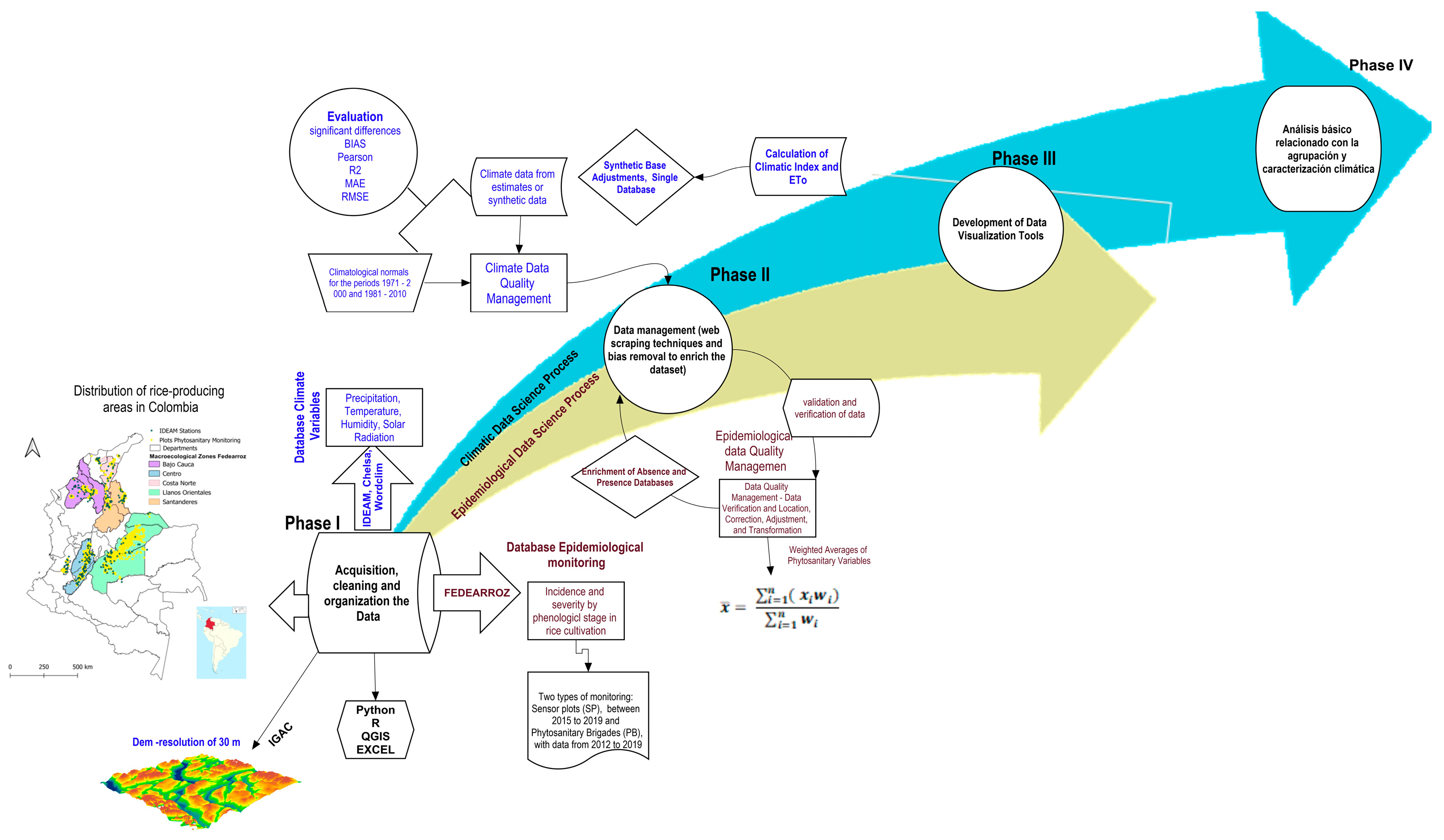
2.1. Description of Approach Used

Our study was based on the application of phases of data science. This comprehensive approach underpinned our study’s methodology, enabling the exploration and interpretation of crucial data pertinent to the phytosanitary data and climatic variables within the context of rice production systems in Colombia (Figure 1).

We implemented three phases. (i) Management, Cleaning, and Organization of Databases: our initial phase involved the meticulous management, cleaning, and organization of databases housing phytosanitary monitoring data and climatic variables within rice production systems in Colombia. (ii) Acquisition of Climatic Data via Web Scraping: in the second phase, we opted to procure a novel set of climatic data through the utilization of web-scraping tools. To achieve this, we accessed spatialized databases of climatological normals obtained from CHELSA and WORLDCLIM (WC). These datasets were subjected to a rigorous evaluation, validation, and adjustment process to rectify any identified biases. (iii) Development of Data Visualization Tools: in the final phase, our focus shifted towards the development of various tools dedicated to the visualization of epidemiological and climatic data. Emphasis was placed on an initial phase of analysis, where a method for ascertaining homologous and heterologous climatic zones was employed. Notably, this classification approach involved unsupervised methods using the spatial K-means algorithm.

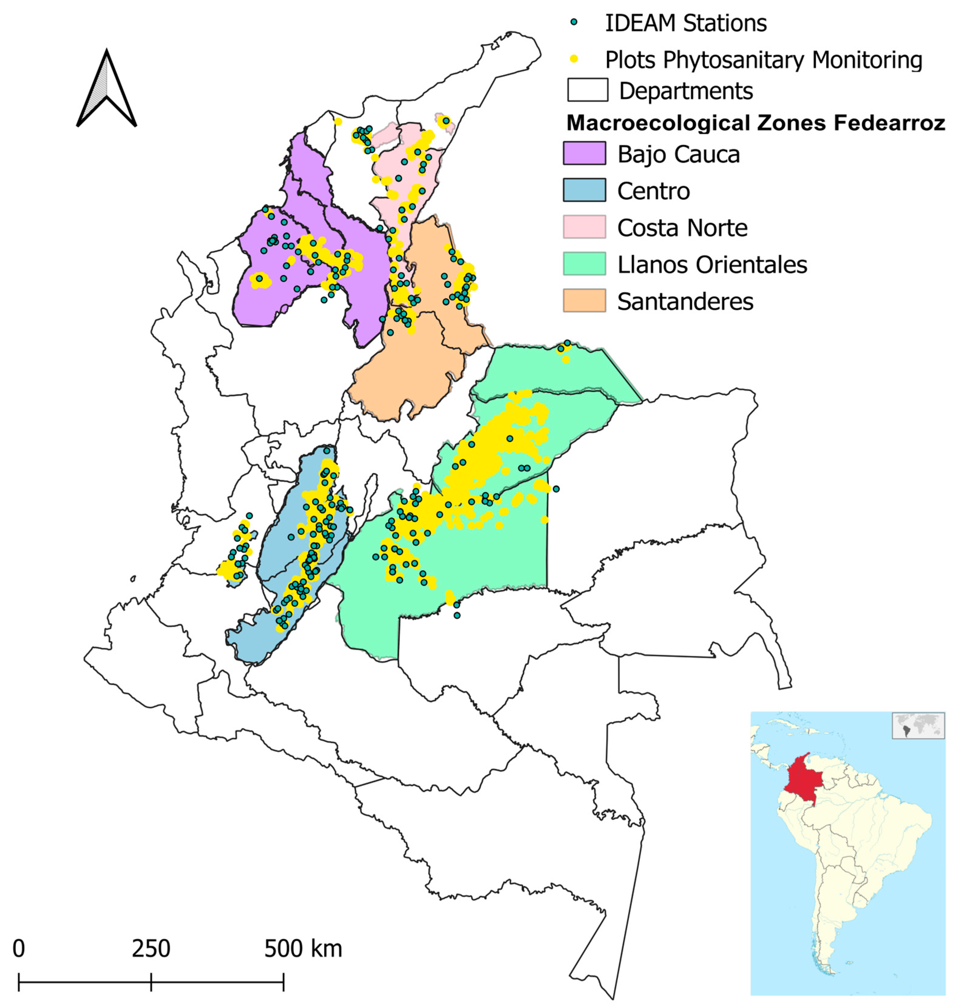
2.2. Basic Description of the Study Zone

The present work was conducted with the data collected from the main commercial rice cultivation areas in Colombia, which were distributed in a large area of the warm zones of the country, and in which the dryland planting system was predominant. Fedearroz classifies the following five areas as rice-growing, given their agrological and geographical conditions: Costa Norte, Santanderes region, Zona Centro (where irrigated rice predominates), Bajo Cauca (where crops are rainfed in most municipalities), and Llanos Orientales, where both systems are present (irrigated and dryland with a predominance of the dryland system) (Figure 2) [27].

The Costa Norte area, considered the “Dry Caribbean”, includes the departments of Atlántico, Cesar, La Guajira, Magdalena, and some municipalities in the department of Bolívar. The Santanderes region includes the rice-growing municipalities of the departments of Norte de Santander and Santander. The Zona Centro includes areas located in the valleys of the Magdalena and Cauca rivers belonging to the departments of Cundinamarca, Huila, Tolima, and to Cauca and Valle del Cauca, respectively. Bajo Cauca, considered the “Humid Caribbean”, includes the departments of Antioquia, Bolívar, Córdoba, Sucre, and some rice-growing municipalities in Chocó. The Llanos Orientales refers to the immense plains just east of the Andes and comprises the departments of Arauca, Casanare, Guaviare, Meta, Vichada, and the municipality of Paratebueno in Cundinamarca (Figure 2) [3,27].

2.3. Part A: Management of Epidemiological Data Associated with the Monitoring of Rice Diseases in Colombia

Information regarding the epidemiological data associated with the monitoring of pathogens that affect rice cultivation in Colombia was provided by Fedearroz, under a collaboration agreement. These data were obtained from the national disease monitoring program conducted on commercial rice plantations, where the producers made management decisions directly. The program included two types of monitoring: (i) sensor plots (SPs), which included data obtained between the period ranging from 2015 to 2019, and (ii) phytosanitary brigades (PBs), with data ranging from 2012 to 2019.

In both types of monitoring, the data were recorded in order to quantify the measures of intensity of the diseases associated with the rice crop, which were estimated based on a field evaluation protocol using quantity parameters, such as number of plants, panicles or leaves affected, size and number of lesions incidence (I), and severity (S) [28,29,30].

SPs consisted of phytosanitary sampling conducted on approximately 145 commercial rice production farms, located in a radius of up to 30 km around the automatic meteorological stations installed by Fedearroz. This network complies with the guidelines of the World Meteorological Organization (WMO) and the protocols of the Institute of Hydrology, Meteorology, and Environmental Studies (IDEAM). Phytosanitary sampling was performed periodically over 7 phenological stages determined in the monitoring protocol by Fedearroz. The stages are (2) sowing to emergence; (3) seedling to the start of tillering; (4) maximum tillering to start of floral primordium; (5) start of floral primordium to start of budding; (6) maximum clogging to start of flowering; (7) flowering with doughy grain; and (8) harvest [29]. For the purposes of the abovementioned points, it was considered that the rice crop was normally inhabited by pathogens; however, there were critical times when they had an economic impact (for more information, see Supplementary Information Table S1) [28]. It should be noted that 26,832 items were processed in the original LS dataset.

PB monitoring was conducted on nearly 2900 commercial rice crops at the end of their production cycles, that is, between phenological stages 7 and 8. PBs is considered a rapid monitoring mechanism that allows the rapid determination of the incidence levels of phytosanitary limitations in the maturation phases and the execution of a regional diagnosis to warn of possible increases or epidemics, and thus formulate prevention or mitigation strategies for the subsequent crop cycle [30].

Sampling was conducted mainly by measuring the incidence of various diseases, in particular, brown spot complex (Sarocladium oryzae, Fusarium spp., and Pseudomonas spp.). The severity of this disease was evaluated (for more information, see the Supplementary Information in Table S2), according to the disease descriptors [28,29,30]. It should be noted that the consolidated PB dataset comprised 19,056 records in the original database. Finally, both datasets were enriched with presence and absence variables, obtained from the original data.

2.4. Data Quality Management and Visualization Tools for Rice Disease Intensity Estimators

The analysis, processing, and visualization of the data were performed using a multiphase method. (i) Cleaning and data quality stage: the validation and verification of data according to the phenological stage were conducted. In this process, the spatial location and homogenization of coordinates were confirmed; when there were missing data, central regions were applied by village and/or municipality where the information was available. Additionally, disease level values were adjusted, removing those that were not true. Missing data for the evaluation dates and phenological stages were estimated, as long as the data for sowing dates, variety, or data for previous stages per farm and year that allowed the estimation were available. (ii) Inclusion of new variables: all pieces of monitoring data were associated with intensity measures, such as presence (1) or absence (0) and incidence, determined as the ratio between the number of stems affected by the disease and the number of stems evaluated and the severity, quantified according to Fedearroz’s internal criteria and protocols, which were previously validated by the technical staff. (iii) With this clean dataset, an exploratory analysis and data visualization using some descriptive metrics were conducted, for which the mean and its graphic representation using the boxplot diagram were used.

In the analysis of the databases, imbalances were identified in the composition of the data, which generated biases attributed to imbalances in the size of the samples obtained for each year, department, variety, and phenological stage. Therefore, the weighted means of the variables were calculated using a weighting parameter specific to each database, considering the weight of each piece of data captured based on its subpopulation by department, year, variety, and phenological stage of the cultivation in which it was monitored. For this process, theoretical bases of the weighting method were used [31]. Equation (1) was used for the calculation:

$$\overline{\mathit{x}}=\frac{{\sum }_{\mathit{i}=1}^{\mathit{n}}{({\mathit{x}}_{\mathit{i}}\times \mathit{w}}_{\mathit{i}})}{{\sum }_{\mathit{i}=1}^{\mathit{n}}{\mathit{w}}_{\mathit{i}}}$$

(1)

$\overline{\mathit{x}}$: where weighted means of the variables. ${\mathit{w}}_{\mathit{i}}$ = corresponds to the weight of each weighting factor (year, department, variety, and phenological stage). ${\mathit{x}}_{\mathit{i}}$ = value of the variable analyzed (incidence and severity).

2.5. Part B: Climate Data Management and Analysis

2.5.1. Management of Data from Weather Stations

A vector-type geographic layer was unified with the coordinates of the plots monitored by Fedearroz, on which circular buffers of 30 km (+/−100 m altitude) were projected for the variables associated with minimum temperature (TMIN), average temperature (TAVE), maximum temperature (TMAX), and potential evapotranspiration (ET), while a buffer of 15 km was projected for precipitation (PCPT). A digital elevation map for Colombia (dem) was used at a resolution of 30 m [32], in which the stations present and the buffer range were validated according to the altitude. The representative area of the meteorological stations was calculated based on the coordinates (latitude and longitude) assuming the sphericity of the Earth and taking as a reference the minimum potential variations of temperature and precipitation as a function of elevation for the low tropical zones [33,34].

Based on the abovementioned ideas, another set of meteorological stations from the IDEAM free dataset (http://dhime.IDEAM.gov.co/atencionciudadano/ (accessed on 1 November 2021)) was established and, with the help of the buffer projections, the stations located within the study area were selected. The data were extracted from climatological normals for the periods of 1971–2000 and 1981–2010 from IDEAM. Subsequently, the precipitation data for both normals were compared to determine whether there were significant differences between the two periods and, where this was the case, these climatologies were specifically analyzed. This process was conducted to guarantee consistency in the weather patterns. To identify changes in the weather and determine whether these were due to errors in the data processing, a comparative analysis with the neighboring climatology was performed. Based on this, we decided to work with the 1971–2000 climatology, which presented the best performance based on the relatively low amount of variation and adjustment needed.

Subsequently, the concept of web scraping was applied to extract the data from the stations located in the previously described buffer zone for the following variables: PCPT, TMIN, TAVE, and TMAX for the periods 1971 to 2000, and ET for 1981–2010. In the case of ET, this period was used because, since the 1981–2010 climatology results, the IDEAM has reported information on this estimated variable. Web scraping consists of a technique in which the data located on freely accessible websites are extracted and stored in a central local database, spreadsheet, or file with multiple extensions. In this process, the URL of the website is used for this purpose, which, in addition to automating the process, has a strong impact on optimization over time and data management [35].

The distribution of the stations was heterogeneous, In accordance with the rice-producing areas in Colombia. The data were used from 214 meteorological stations for PCPT, 227 stations for ET, and 82, 84, and 79 stations for TMIN, TAVE, and TMAX, respectively. The stations consulted for each variable are foupresentednd in the Supplementary Materials associated with Table S4.

2.5.2. Management of Climate Data from Estimates or Synthetic Data

Two synthetic climate datasets were validated, namely, (1) Climatologies At High Resolution For The Earth’s Land Surface Areas, known as CHELSA V 2.1 [15], and (2) Global Climate Data, known as WORLDCLIM V 2 (WC) [15]. This was performed with the aim of enabling the use of the climatic data of variables at fine spatial resolutions (~1 km) for the climatic characterization of rice zones based on clustering and on the determination of homologous and climatically heterologous zones that are described in later sections.

CHELSA is an estimated dataset that originates from downscaling the ERA-Interim climate re-analysis to a 1 km resolution [14]. To improve the resolution, precipitation accuracy, and downscaling, orographic predictors, including wind fields, valley exposure, and boundary layer height were incorporated, with subsequent bias corrections. The resulting data consist of monthly time series of temperature and precipitation over the period of 1979–2018 [36]. Meanwhile, WORLDCLIM V 1.4 corresponded to a set of average monthly interpolated climate data from meteorological stations on a multi-resolution grid [37]. Its origin is based on a dataset that consists of the precipitation records of 47,554 locations, average temperatures for 24,542 locations and minimum, and maximum temperatures for 14,835 locations; in all cases, the locations were distributed around the world [15,37]. In version 2.1, it was refined to include additional stations, other factors, such as cloud cover and distance to the ocean, and high-resolution datasets on vapor pressure [15].

Data extraction from both data sources was performed using Worldclim V2.1 and CHELSA V2.1 web-scraping methods for the multi-year monthly climatologies for 1971–2000 and 1981–2010, respectively, and for the IDEAM stations in the same location. The selected meteorological variables were PCPT, ET, TMAX, TAVE, and TMIN.

2.6. Evaluation of the Quality of Climatological Data from Estimates vs. In Situ Data

A comparative analysis was conducted between the two synthetic datasets with those observed in situ of the climatological normals. In the realm of data analysis, assessing and comparing the quality of different data sources is of paramount importance. Various metrics have been developed to facilitate this process, allowing analysts to gain an insight into the degree of variation and approximation between datasets. For this, significant differences were analyzed, and the error of the differences was subsequently calculated. For this purpose, five different metrics were calculated and used to validate the estimated data. (i) Pearson’s correlation coefficient (r), which establishes the relationship between the observed and estimated data, is a widely used metric that quantifies the strength and direction of the linear relationship between two variables; it provides a measure of how closely their data points are aligned [38]. (ii) Coefficient of determination (R²), in which the best possible score is 1.0 and can be negative when the estimation model is arbitrarily worse [39], is used to establish the proportion of variation explained. In the context of comparing two data sources, a high R² value indicates that one dataset is a good predictor of the other, while a low value suggests a poor fit. (iii) BIAS calculates the differences between the estimate (data from Chelsea and Worldclim) and true value (in situ data); it is a metric that evaluates the systematic errors or discrepancies between two datasets. It provides insights into the overall deviation between the datasets, which may arise from measurements or the data collection values processed [40]. (iv) Mean absolute error (MAE) is a metric that quantifies the average magnitude of errors between two datasets. It provides a measure of the absolute differences between corresponding data points in the datasets. A smaller MAE indicates less variations or errors between the datasets, while a larger MAE suggests a greater dissimilarity [41]. (v) Root mean square error (RMSE) accounts for both the magnitude and spread of errors, providing a more comprehensive evaluation of variation. Lower RMSE values indicate a greater similarity between datasets, while higher values signal a greater dissimilarity, the last of which is very sensitive to the presence of extreme items in the data [41].

By analyzing the performance of the datasets, it was established that CHELSA should be used for the PCPT and ET variables and WC for TMIN, TAVE, and TMAX. However, it was necessary to calculate a simple linear regression model to adjust the variables selected and estimated by WC, based on the error of differences with the data from the multi-year monthly observations recorded by the IDEAM. To this end, the parameters used to make the adjustment and correction of the bias were those associated with the equation of the regression model line (Equation (2)). The adjustment factor was obtained per station and applied to all the data extracted from WC that were within a radius of influence of 30 km from each station. Once the adjustment was performed, the normals were unified to apply them to the clustering. In cases in which there was no influence station, they were not adjusted, taking the extracted data for the cluster analysis.

$$\mathit{Y}=\mathit{\beta }0+\mathit{\beta }1\mathit{X}1+\mathit{\epsilon }$$

(2)

where $\mathit{Y}$ corresponds to the multi-year monthly value of the variables observed in situ; $\mathit{X}1$ to the monthly multiannual value of WC; $\mathit{\beta }1$ to the adjustment factor for each station, which is multiplied by the $\mathit{X}$ value; and $\mathit{\beta }0$ to the adjustment value, called the y-intercept, which is added to the value of BX to obtain the $\mathit{Y}$ value.

To achieve a better climate characterization, the PCPT, ET, and temperature data, previously validated and adjusted, were complemented with other climatological variables obtained from estimated datasets that were considered to be of agricultural and phytosanitary importance for the purposes of the study (

Table 1. Meteorological variables extracted from the CHELSA and WORLDCLIM datasets.

Variable	Abbreviation	Physical Unit	Period	Periodicity	Source
Precipitation	PCPT	mm	1981–2010	Monthly multiannual	CHELSA
Minimum temperature	TMIN	°C	1971–2000 (WC) y 1981–2010 (CH)	Monthly multiannual	CHELSA and Worldclim
Average temperature	TAVE	°C	1971–2000 (WC) y 1981–2010 (CH)	Monthly multiannual	CHELSA and Worldclim
Maximum temperature	TMAX	°C	1971–2000 (WC) y 1981–2010 (CH)	Monthly multiannual	CHELSA and Worldclim
Solar radiation	RSDS	MJ m−2 d−1	1981–2010	Monthly multiannual	CHELSA
Evapotranspiration potential (Penman–Monteith)	ET	mm	1981–2010	Monthly multiannual	CHELSA
Relative humidity	RH	%	1981–2010	Monthly multiannual	CHELSA
Vapor pressure deficit	VPD	hPa	1981–2010	Monthly multiannual	CHELSA
Total cloud cover	TCC	%	1981–2010	Monthly multiannual	CHELSA

). Likewise, the calculation of two indices was included: (i) the aridity index [42,43], which expressed the relationship between PCPT precipitation and ET potential evapotranspiration obtained by the Penman–Monteith method, and (ii) an index based on the equations and the methodological report described by [44]. From the mathematical expressions, the thermal oscillation index was proposed, which enabled the elucidation of the oscillation of temperatures, calculated as a difference in maximum and minimum temperatures, normalized with the average temperature (Equation (3)):

$$\mathit{T}\mathit{h}\mathit{e}\mathit{r}\mathit{m}\mathit{a}\mathit{l} \mathit{o}\mathit{s}\mathit{c}\mathit{i}\mathit{l}\mathit{l}\mathit{a}\mathit{t}\mathit{i}\mathit{o}\mathit{n} \mathit{i}\mathit{n}\mathit{d}\mathit{e}\mathit{x} = \frac{\mathit{T}\mathit{M}\mathit{A}\mathit{X}-\mathit{T}\mathit{M}\mathit{I}\mathit{N}\mathrm{}}{\mathit{T}\mathit{A}\mathit{V}\mathit{E}}$$

(3)

Within the proposed methodological process, the coherence of the magnitudes and spatial variability of the variables RSDS, RH, VPD, and TCC were validated. However, their performance was not analyzed with respect to the in situ data, since, in order to conduct this analysis, complete series (30 years or more) were required and, when reviewing the IDEAM data, the stations available with, for example, the solar radiation variable, had data available for 20 years or less [45]. Regarding the other variables, when these were estimated, a bias could have occurred due to the methodology, missing data, and errors inherent in the process that could have affected the performance analysis.

2.7. Practical Application of Climate Data Management: Agroclimatic Zoning for Rice-Producing Regions in Colombia

Each plot evaluated within the Fedearroz phytosanitary monitoring program was assigned the values of the climatological normals of the variables originating from the estimated datasets (Table 1), which were previously unified and adjusted. This was performed to facilitate the classification of homologous or heterologous rice-producing areas, based on their agro-climatic characteristics, making it possible to group the data analysis and find the relationships between the distribution of pathogens and climatic characteristics that determined each area.

Based on the analyses performed, it was established that the datasets should be used in combination to perform climate clustering. Therefore, an adjusted WC was used for temperatures (minimum, average, and maximum) and CHELSA for the other variables. Considering the analyses conducted, the estimated climate datasets constituted an option for performing spatial analyses of homogeneous areas, after validating the data and adjusting them if technically feasible.

It was proposed to conduct this classification because, in the rice production sector in Colombia, there is currently no zoning of producing regions based on agroclimatic characteristics and multiple variables. The current zoning applied by the rice-growers’ union is empirical and considers some geographical characteristics, as shown in Figure 1. The determination of climatic homologous zones is a concept that has been applied with the objective of characterizing climate at a macroscale (region, country, and other levels), thus being able to identify multiple important phenomena, such as climate risk zones, differential impact of climate variability and change phenomena, and optimal areas for planting plant species [46,47]. This analysis was conducted under multiple approaches, such as multivariate statistics and machine learning based on unsupervised classification tools, where the use of the K-means algorithm was widespread [46,47].

In our work, the clustering methodology used by [48] was taken as a reference, with some variations considered basic to improve the methodological adjustment. Multivariate statistics were used in a multistage process as follows. (i) Application of principal component analysis (PCA) to determine the important agroclimatic variables in the classification and grouping of producing areas (Table S3). In addition, PCA could be used to enable us to graphically elucidate the variation explained by the components and their interrelationship with the clusters employed in our analysis. PCA is a statistical procedure that seeks to reduce the dimensionality of a dataset by calculating new variables called principal components as linear combinations of the original variables [49]. (ii) To group the areas (homologues and heterologous zones based on climatic varication), a cluster analysis was performed, a process based on the differences of various types of objects and that uses distance regulation functions to produce unsupervised classification models [50]. For this, the K-means grouping method was implemented in the sklearn library run in the Colab Python environment [51]. This method consists of an algorithm that separates a set of data into k groups based on the distance between the data and the central regions of the groups [52]. This produces a separation of the objects into groups from which the metric to be minimized can be calculated [52]. K-means is a widely recognized and employed method for its suitability for climate clustering [46,47]. The use is supported by the following key justifications: simplicity and speed, interpretability, scalability, proven effectiveness, flexibility in number of clusters (K), robustness, and availability in tools and libraries [52,53]. In addition, for this process, the cluster number to be determined is a critical factor for obtaining good results. Therefore, to establish the grouping criterion, the elbow method was applied, which consisted of examining the percentage of variance explained based on the number of clusters [54]. The “elbow method” is a widely used technique in data analysis and clustering to determine the optimal number of clusters (K). The process involves executing the K-means algorithm with a range of K values, typically from 1 to a predetermined upper limit [54]. For each K value, the algorithm computes the sum of squared distances (often referred to as the within-cluster sum of squares between data points and their assigned cluster centroids) [54]. Subsequently, once the clusters were generated, the clusters were spatially projected onto the rice-producing areas. This process was validated by the Fedearroz technical team, confirming that the analytical process agreed with the empirical groupings, but with a higher spatial resolution and with the general climatic classification of the rice-producing areas in Colombia. (iii) Finally, for each cluster, the attributes of the agroclimatic variables that were important for the climatic characterization that determined each cluster were described.

2.8. Basic Analysis of the Information, Libraries, and Software Used

When considering the large amount of data and the option of obtaining variables derived from these and other sources for the purpose of this study, a data science approach was applied (outlined in the Introduction). For this, several tools were applied to clean, visualize, and analyze the data. The free software Python 3.12.0 was used in the Colab, Visual Studio Code, and Spyder environments. Specific functions of the Pandas libraries were applied for data management, Numpy was used for numerical calculations and the data analysis, Matplotlip for the creation and customization of graphs, and Sklearn [51] as a machine learning and statistical modeling tool. This last library was applied to perform a regression analysis, error analysis, grouping, and dimensionality reduction. Additionally, to manage the geographic data, the free software Qgis 3.16.6 [55] was used to extract gridded data and spatialize the evaluated variables.

3. Results

3.1. Data Gestion Tools Used

Our results present the advantages of data science tools’ implementation, specifically tailored for the management of data stemming from phytosanitary monitoring and climatic stations. This meticulous process enabled us to assess data quality, identify and eliminate outliers, address missing data, compute new variables, and efficiently concatenate databases, among other essential tasks. To achieve this, we harnessed the power of various open source library functions designed for Python and executed them across diverse environments.

The workflow we implemented proved to be a game changer, as it facilitated a swift, accurate, and partially automated data management process. This efficiency was made possible by harnessing the numerous advantages offered by tools available in libraries, such as Pandas, Matplotlib, Numpy, Plotly, Seaborn, Sklearn, and others. Our utilization of these resources not only expedited data handling, but also enhanced the precision of our analysis, ultimately contributing to the robustness and reliability of our findings.

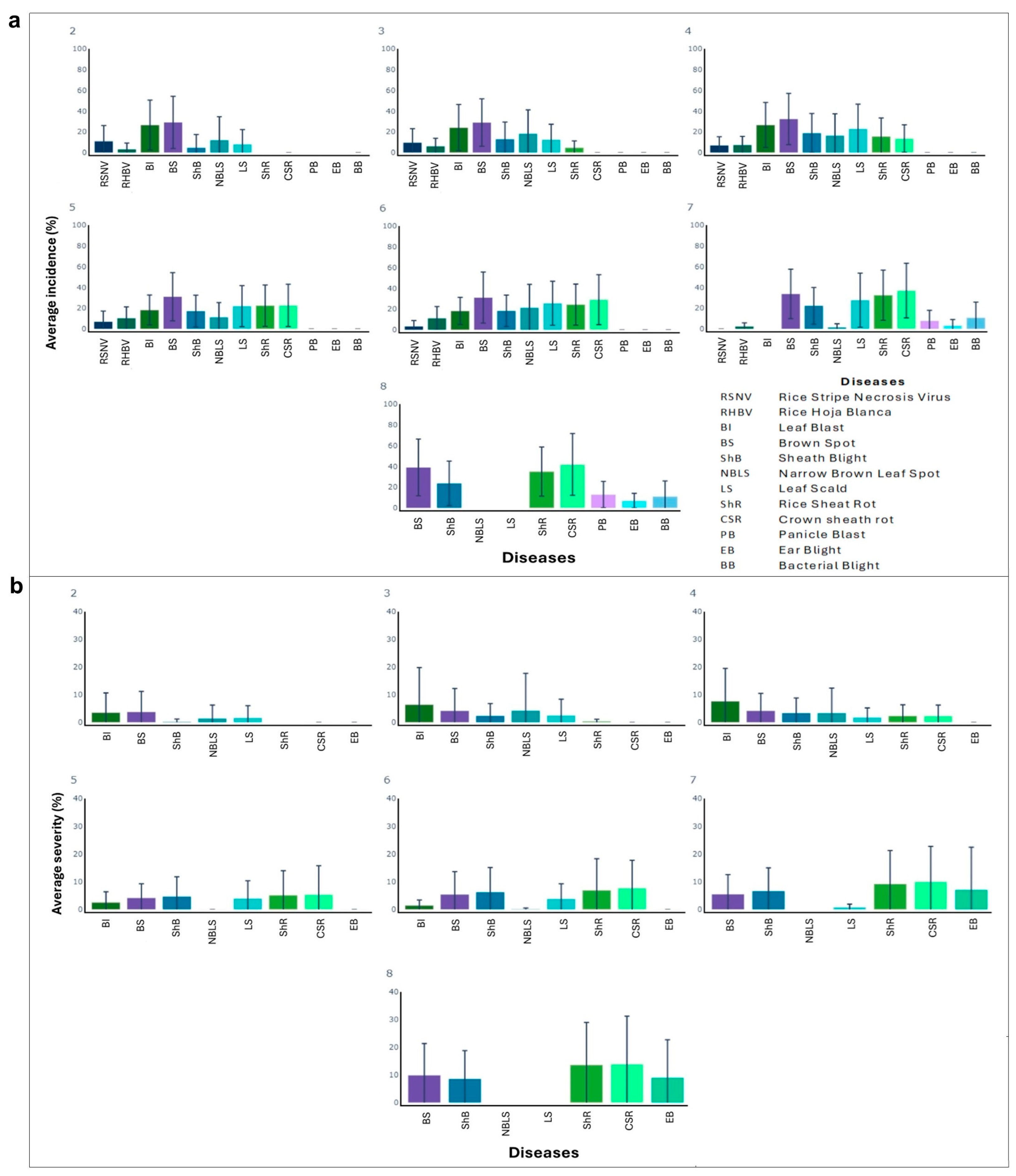
3.2. Part A: Data Quality Management and Visualization Tools for Rice Disease Intensity Estimators

A descriptive analysis of the epidemiological data associated with the SP and PB monitoring programs was performed. It was observed that, in 2016, a greater number of samplings were conducted and, consequently, an increase in the presence of diseased plants was observed compared to the other years analyzed (Figure S1). The abovementioned results occurred due to the implementation of a special monitoring program, which allowed the sampled population to increase in that year. By using the boxplot diagram as a visualization tool, it could be validated that medians close to zero predominated in most diseases and there was a high deviation and variation of the data considering the amount of extreme data (Figure S2).

The visualization based on the weighted means of the data from SP indicated that, during all phenological stages, the disease with the highest incidence was brown spot (BS), with values between 35% and 40%, followed by leaf blast (BI), which, from stages 2 to 6, presented incidences between 18% and 28%. During the stages considered as reproductive, specifically 5 to 8, the most relevant diseases in addition to BS were crown sheath rot (CSR), BS, rice sheath rot (ShR), and leaf scald (LS), with incidences between 18% and 40% (Figure 3a).

Regarding the average severity of the diseases evaluated in the SP program, the results indicate that BI on leaves presents the highest levels, with values between 4% and 8% during stages 2 to 4. Meanwhile, in the reproductive stages 5 to 8, the BS, rice sheath rot (ShR), and CSR diseases present severities between 8% and 15%, and grain spot between 7% and 10% (Figure 3b).

3.3. Part B: Management of Climatological Data from In Situ and Estimated or Synthetic Stations

When comparing the climatological normals of precipitation for the periods of 1971–2000 and 1981–2010 from in situ stations, consistency in the values and patterns of precipitation were found in most of the stations. Specifically, in 96.3% of the analyzed stations, the R² was greater than 80%, and in 97% the r was greater than 0.9 (Figure 4a,b). However, six stations were identified that, in the climatological period of 1981–2010, presented anomalies with respect to the period of 1971–2000, which physically did not maintain the precipitation patterns of those areas with respect to the predominant large-scale atmospheric circulation. This behavior was evaluated with the R² statistics, whose value tended to be 0, while that of r was less than 0.2 (Figure S3a,b). Additionally, regarding the analysis of the error metrics, an average of the RMSE and MAE was obtained for the precipitation variable between 10 to 12 mm, with more than 50% of the data being less than 11 mm (Figure S3c).

With respect to the estimated or synthetic data, the spatial distribution of the values of the variables extracted from the datasets for the study area was analyzed. As expected, a decrease in the temperature with an increasing altitude was evident. CHELSA reproduced lower minimum and maximum temperature values than WC for the study area. Regarding the precipitation in the distribution maps, there are important differences between CHELSA and WC, which can be attributed to the origin of the data, the estimation method, the related variables, the bias corrections, or other factors (Figure 4c,d).

For the specific study area (rice-producing areas in Colombia), the satisfactory performance of the annual values of the evaluated datasets was presented, considering the values of r and R². When comparing the estimated precipitation with respect to observations from in situ stations, R² values of 0.70 and 0.72 were obtained with the data from the CHELSA and WC sources, indicating that the variation of the observed annual PCPT correlated with the estimated variation. Regarding the minimum, average, and maximum temperatures, an acceptable performance was observed for both datasets, with R² values between 0.65 for TMAX estimated with CHELSA, and 0.84 for the same variable with WC (Figure 4a,b). Meanwhile, the ET estimated by CHELSA had the worst performance, with an R² of 0.02 (Figure 4a).

In general, it was observed that the datasets preserved, in most of the points compared, the seasonality of the climatologies of precipitation, evapotranspiration, and temperature. It is important to highlight that CHELSA tends to represent the rainiest areas in the country better than WC. This includes locations in the Pacific and Orinoquía regions, as well as in the Amazon foothills, among other regions, whose annual rainfall ranges between approximately 4000 and 11,000 mm. (Figure 4c). Meanwhile, WC better represents temperature values, since CHELSA tends to represent lower values in this variable (Figure 4d).

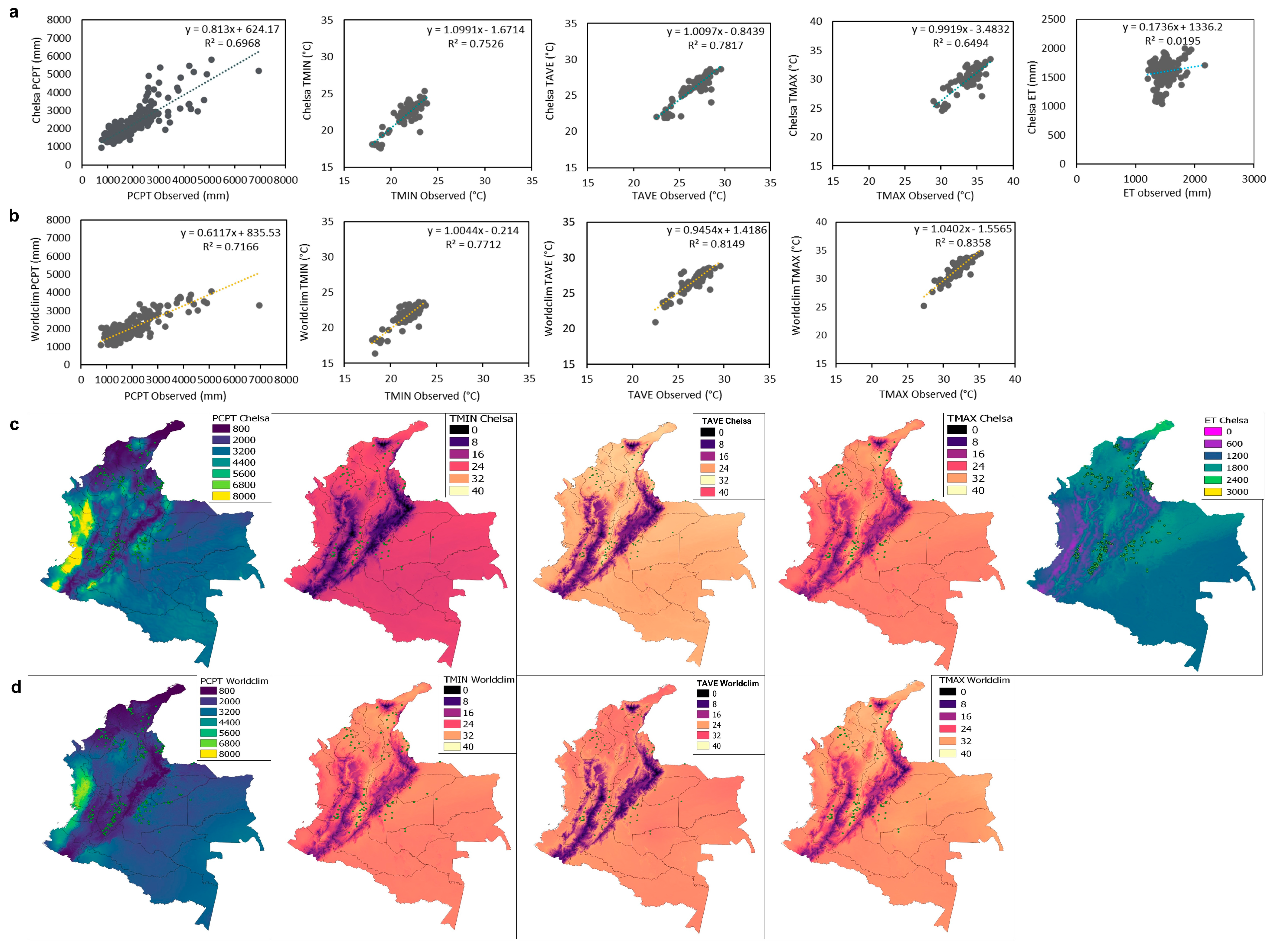
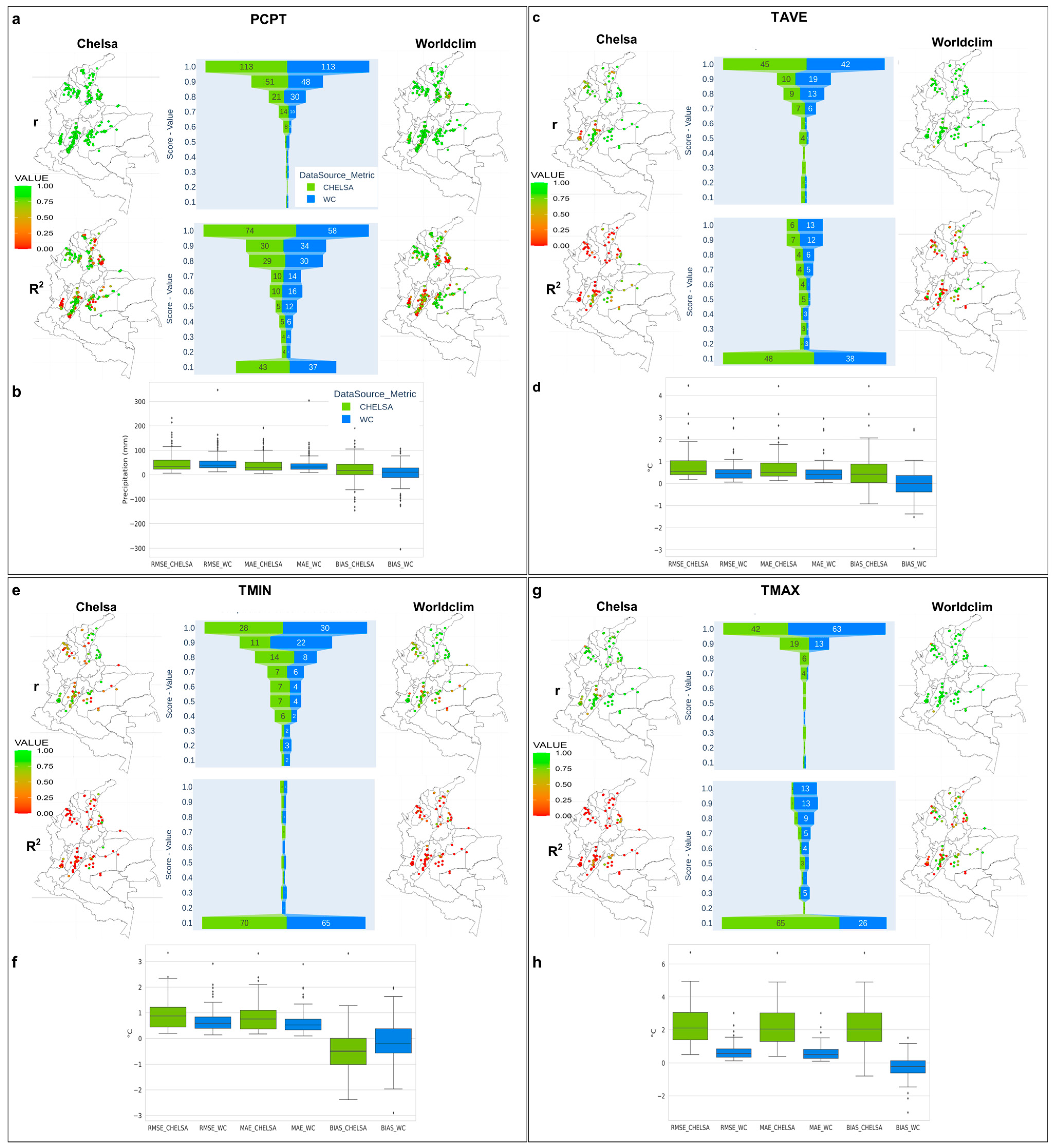
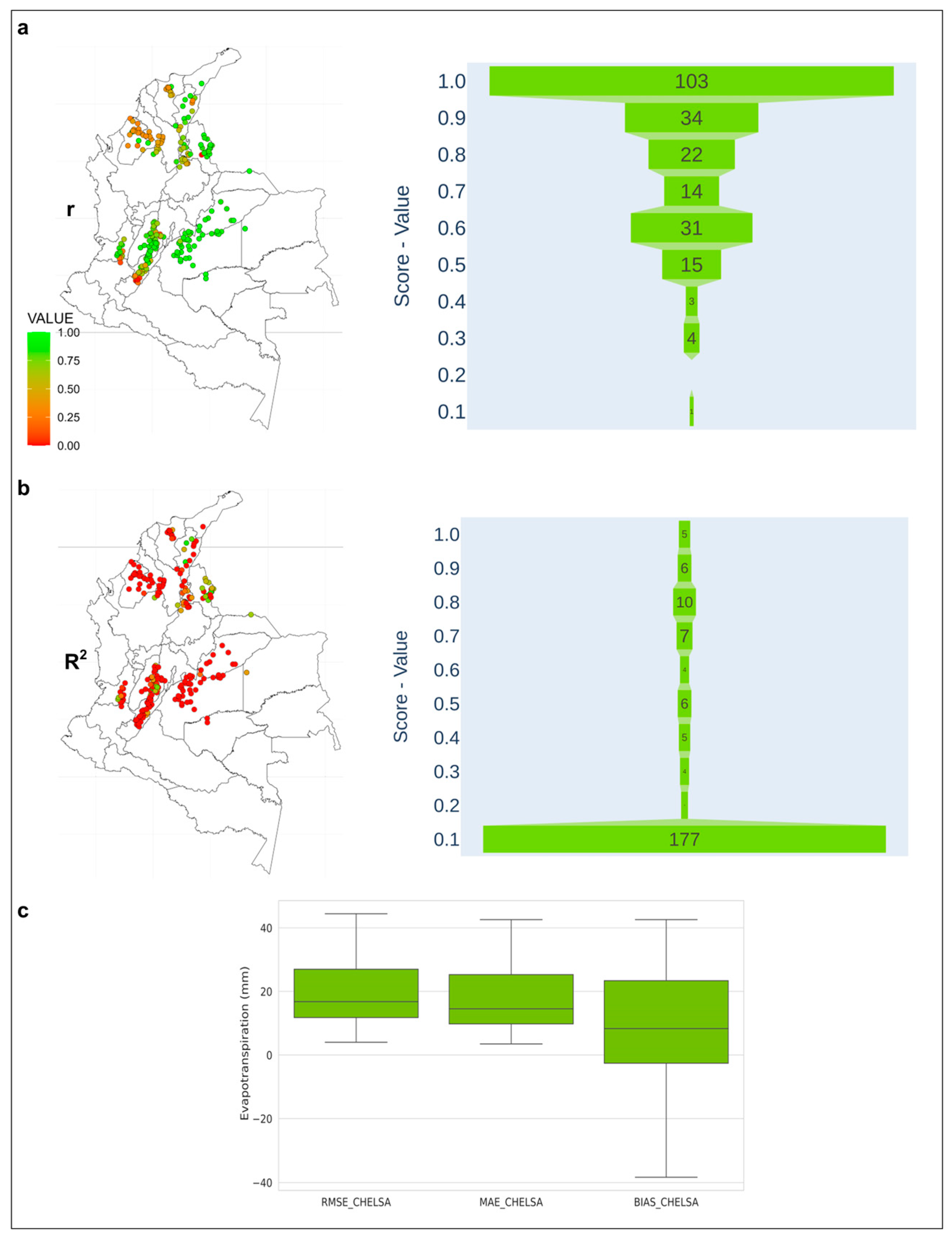
3.4. Evaluation of the Quality of Climatological Data from Estimates vs. Data from In Situ Stations

When analyzing in detail the comparison of the values of the monthly PCPT climatologies between the stations (214 in total), it was found that CHELSA presented an R² ≥ 0.70 for 66.8% (143) and WC for 63.5% (136) of the stations. Meanwhile, the r was greater than 0.7 for 93% (199) of the stations evaluated for CHELSA and for 94% (201) for WC (Figure 5a). However, the bias values were between −143 to 196 mm with an approximate mean of 20 mm for CHELSA and 13 mm for WC (Figure 5b). At a general level, the error values are acceptable, considering that different methodological processes may occur in the calculation of climatological normals, as a result of aspects related to the characteristics of the time series, number of observations, missing data, and errors in the recording and processing of the data. Meanwhile, the extreme data reported in the metrics are due to the stations that present anomalies between the climatological normals.

When analyzing the monthly behavior and seasonality of temperatures (minimum, average, and maximum) estimated by the datasets with respect to the observed data, it was evident that WC presented a better approximation than CHELSA, considering the following results for each variable: TMIN estimated by WC presented an R² ≥ 0.7 for 9.5% (8) of the stations, while in CHELSA, the corresponding figure was 10.7% (9) (Figure 5e). However, r ≥ 0.7 occurred in 72.3% (60) of the stations for CHELSA and in 79.5% (66) for WC (Figure 5e). TAVE, on the other hand, had an R² ≥ 0.7 for 25% (21) of the stations evaluated for CHELSA and 42.85% (36) for WC. Values of r ≥ 0.7 were presented in 84.5% (71) of the stations for CHELSA and in 95.23% (80) for WC (Figure 5c). Regarding the TMAX, the WC estimation was obtained for 50.6% (40) of the stations with R² ≥ 0.7, while CHELSA had this level of the coefficient in only 8.86% (7) of the evaluated stations. In this regard, for estimates of the variable in CHELSA, 89.87% (71) of the stations presented r ≥ 0.7, and with WC, the corresponding figure was 97.5% (77) (Figure 5g).

The analyses of the RMSE and MAE error metrics used confirm that CHELSA presents a worse performance than WC, in relation to TMIN, TAVE, and TMAX (Figure 5d,f,h). Specifically, for the TMIN variable estimated by CHELSA, the values of MAE and RMSE both range between 0.18 and 3.34 °C with an approximate average of 0.89 °C, while for the estimates with WC, they are between 0.10 and 2.92 °C, with an average of 0.68 °C (Figure 5f). For TAVE, the value of the errors is between 0.13 and 4.45 °C, with an approximate average of 0.80 °C, while WC presents values between 0.04 to 2.96 °C, with an approximate average of 0.5 °C (Figure 5d).

The values evaluated for TMAX with CHELSA present a magnitude of errors between 0.35 and 6.7 °C, with an average of 2.3 °C, while with WC, the values are between 0.1 and 3 °C, with an average value of 0.6 °C (Figure 5h). Regarding bias, the value of this for TMIN estimates was between −2.38 and 1.95 °C, with an approximate mean of 0.3 °C for both datasets (Figure 5f). The TAVE values were between 1.5 and 2 °C, with an approximate average of 0.27 °C (Figure 5d). The TMAX estimates had a greater magnitude bias, especially with CHELSA, where it was between 0.8 and 6.7 °C with a mean of 2 °C, while for WC, this was between −3.0 and 1.5 °C with a mean of −0.2 °C (Figure 5h).

When evaluating the estimation of the ET data for CHELSA with respect to the observed data, it was evident that the estimated ET for most of the stations presented an R² around 0.1 (Figure 6b). However, r ≥ 0.7 occurred in 70% (159) of the stations (Figure 6a). The analyses of the RMSE and MAE error metrics used indicated that CHELSA presented a worse performance, given that the MAE and RMSE values ranged between 4 and 40 mm with an approximate average of 18 mm, while the BIAS ranged between −38 and 42 mm (Figure 6c).

To obtain a better performance and enable the use of the WC temperature estimates, adjustment factors based on linear regression were calculated and applied to the temperature values and thus reduced biases. When conducting this process, it was observed that the adjusted WC presented a better approximation than the initial WC. Specifically, the following results were obtained for each variable: TMIN for adjusted WC presented an R² ≥ 0.7 for 63.4% of stations (52 in total) (Figure 7a); for TAVE, R² ≥ 0.7 for 99.2% of the evaluated stations (75) (Figure 7c); and, finally, for TMAX, R² ≥ 0.7 was obtained for 90.4% of the stations (76) (Figure 7e).

In addition to the results obtained, when evaluating the performance of the adjusted WC, it was found that the bias tended to zero (0) and the errors were reduced for all variables (Figure 7b,d,f). The values of the RMSE and MAE metrics for TMIN were between 0.06 to 0.5 °C, with an approximate mean of 0.18 °C (Figure 7b). In TAVE, the values of both metrics ranged between 0.03 to 0.4 °C with an approximate mean of 0.15 °C (Figure 7d). For TMAX, they were between 0.06 to 0.5 °C, with a mean around 0.2 °C (Figure 7f).

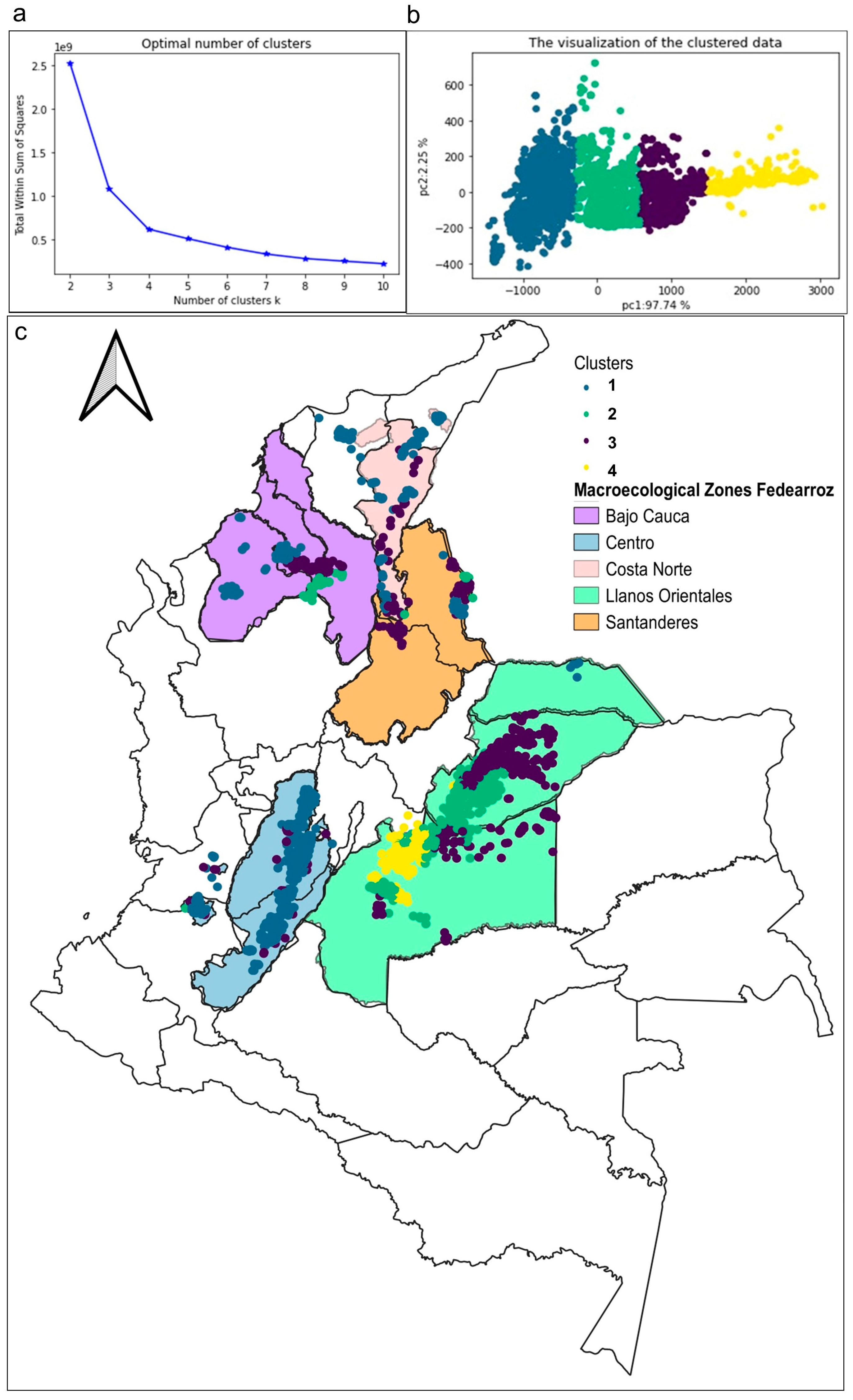
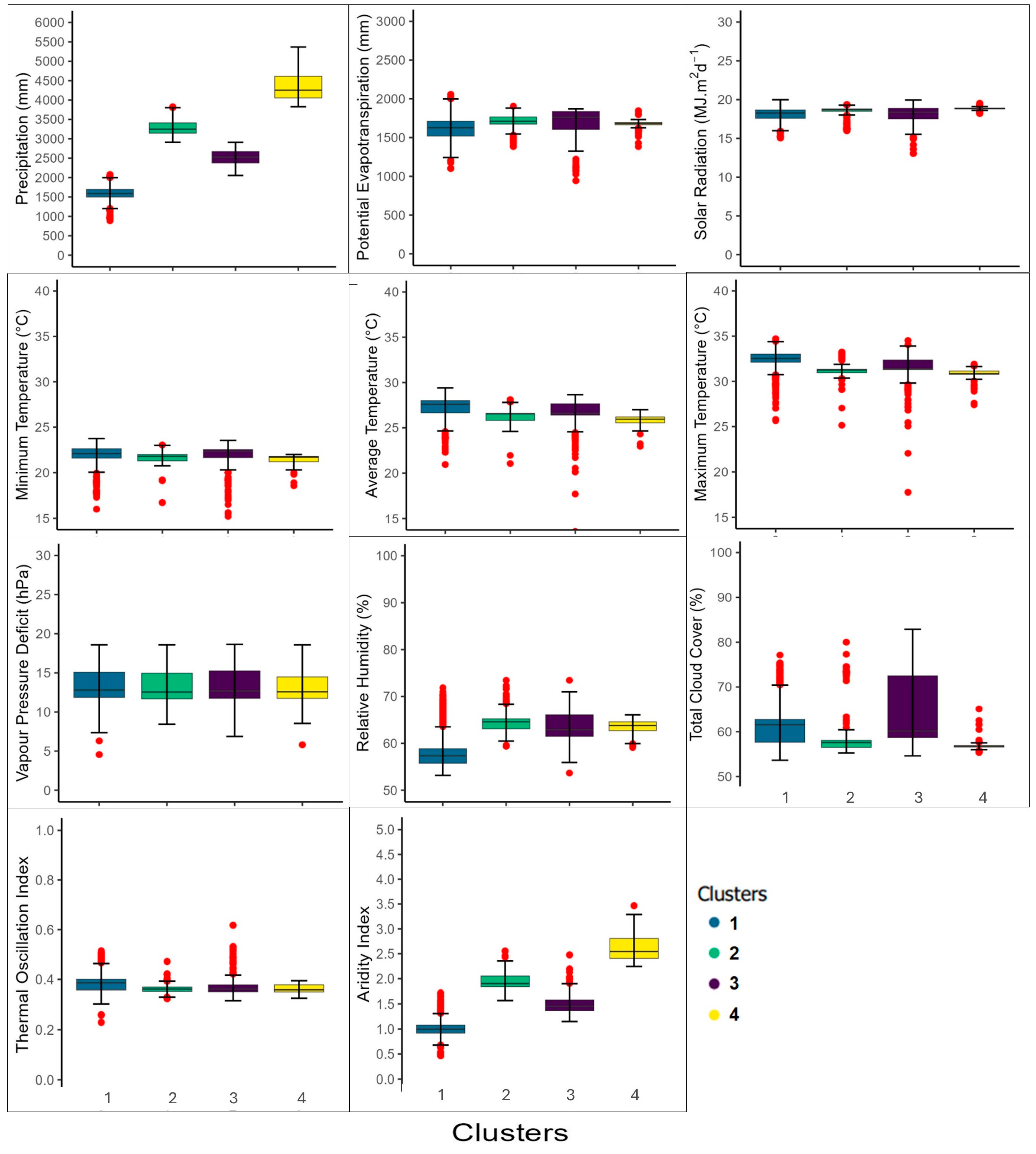
3.5. Agroclimatic Zoning for Rice-Producing Regions in Colombia

Based on the elbow method, it was determined that the optimal number of groups, or the climatic cluster, for the rice-producing areas in Colombia was four, when considering the climatic variables evaluated (Figure 8a). It was found that the first component, composed mainly of the precipitation and annual accumulated evapotranspiration variables (Table S3), explained 97.7% of the climatic variance of these areas (Figure 8b), observing a high variability in these two variables for each climatic cluster (Figure 9), which allowed groupings of climatically homologous zones based to their specific characteristics to be generated.

Cluster 1 includes plots at altitudes between 2 and 1253 m above sea level, located mainly in the northwest, termed Bajo Cauca by Fedearroz, in the north of the Caribbean region and in a large part of the Zona Centro (Figure 8c). These regions are characterized climatically by presenting the lowest annual accumulated PCPT, with values between 700 and 2200 mm per year (it should be noted that these areas may present a difference in the distribution of annual rainfall, which was not considered), with an aridity index between 0.5 and 1.8. In this area, the TMAX ranges between 26 and 35 °C, and the TMIN between 21 and 29 °C. The ET is between 1100 and 2100 mm per year, RSDS between 15 and 20 MJ m⁻² day⁻¹, and DPV between 5 and 18 hPa (Figure 9).

Cluster 2 includes plots with altitudes between 20 and 1370 m above sea level, located mainly in the Llanos Orientales, southern Bajo Cauca and eastern Santanderes (Figure 8c). The accumulated annual PCPT ranges between 2800 and 3800 mm per year, with an aridity index between 1.5 and 2.5, TMAX ranging between 25 and 33 °C, TMIN between 17 and 22 °C, ET between 1300 and 1800 mm per year, RSDS between 16 and 19 MJ m⁻² day⁻¹, and DPV between 8 and 18 hPa (Figure 9). Cluster 3 is composed of plots that are at altitudes between 12 and 1450 m above sea level, located mainly north of the Llanos Orientales, which includes a large part of the department of Casanare, eastern Meta, and some small areas in Bajo Cauca and Costa Norte (Figure 8c). This group presents an annual accumulated PCPT that ranges between 2000 and 3000 mm per year with an aridity index between 1.2 and 2.5, TMAX between 25 and 35 °C, TMIN between 15 and 23 °C, ET between 900 and 1800 mm annually, RSDS between 12 and 20 MJ m⁻² day⁻¹, and DPV between 7 and 18 hPa (Figure 9)

Finally, cluster 4 is at altitudes between 178 and 790 m above sea level, located mainly in what is known as Piedemonte Llanero, in the department of Meta (Figure 8c). It presents the highest annual accumulated PCPT, which ranges between 3800 and 5400 mm annually, with an aridity index between 2.5 and 3.5, TMAX between 27 and 32 °C, TMIN between 18 and 22 °C, ET between 1300 and 1800 mm annually, RSDS between 18 and 20 MJ m⁻² day⁻¹, and DPV between 8 and 18 hPa (Figure 9).

4. Discussion

4.1. Management of Epidemiological and Climatic Data in Rice Production Systems

We were able to have versatile and automated elements for the collection, storage, processing, and evaluation of large-scale data through the application of a multiple set of data science tools in a responsible way and under a step-by-step protocol. This, in turn, enabled agile and timely analyses and decision-making behavior in the context of the phytosanitary and comprehensive management of rice cultivation based on the integration of epidemiological and climatological monitoring. This new field represents an excellent opportunity, given its applicability in basic sciences, such as atmospheric and applied sciences, including agrometeorology, agronomy, and especially in epidemiology, where advances have been achieved with excellent results [53,56].

Data management for epidemiological information in rice cultivation enabled the identification of temporal patterns and phenology based on the levels of incidence and severity for the period of analysis, allowing us to validate that, although pathogens were present throughout the crop cycle, their impact occurred at critical periods [28]. In this regard, the reproductive and maturation phases increased the intensity of diseases, such as BS, CSR, and ShB, while in the vegetative period, there was an increase in BI, a finding that is consistent with previous reports [57]. It is important to highlight that the results obtained show the intensity values of the different pathologies evaluated, which does not necessarily mean that they are the diseases that have the most economic importance, given that, in many cases, the producer performs the strict control of those pathologies that have a potential to damage crops and cause losses. An example that illustrates this point is BI on the leaf and stem, which is considered the disease that most significantly limits the crop [58].

On the other hand, the evaluation of the estimated datasets from the CHELSA and WC sources showed that the rainiest areas of the country, especially the Pacific and Orinoquía regions, and areas of the Amazon foothills close to the Andes Mountain range were best represented by CHELSA. This may have been because this database captured the topographic heterogeneity of precipitation at small scales and showed a more consistent relationship between the terrain and the resulting precipitation patterns, while for WC, it produced poor correlations between elevation and precipitation [14]. These results coincide with those reported in [59].

Regarding the temperature represented by the datasets, TAVE values of around 27 °C can be observed in the rice-growing areas, especially the Llanos Orientales, Costa Norte, and Santanderes regions, which match the findings of [60]. This indicates that these regions present a homogeneous relief, composed mainly of extensive cultivated grass savannahs, especially in the Llanos Orientales. Due to the abovementioned points, the distribution of the average air temperature was very uniform, presenting values that varied around 25 °C.

The r for the PCPT presented values above 0.7 for both sets of data estimated at most observed points. However, the behavior of R² indicated that, depending on the location and dataset, the values tended to be overestimated or underestimated, thus generating biases, given that said coefficient was considered hypersensitive to external values and insensitive to additive and proportional differences between the model predictions and measured data, as established by [61].

The synthetic databases evaluated mostly maintained the seasonality of the meteorological variables analyzed (PCPT, ET, TMIN, TAVE, and TMAX). Regarding the PCPT from CHELSA, this presented better behavior in terms of monthly magnitudes, although it presented slightly higher errors and biases than WC, This was because, whether the variable was calculated or measured indirectly for both CHELSA and IDEAM, there may have been aspects related to the characteristics of the time series, number of observations, missing data, and errors in the recording and processing of the data, which generated a greater bias between estimation and observation values.

CHELSA 2.0 based the data for this variable on ERA5, including orographic wind effects, combined the height of the planetary boundary layer to approximate the orographic effect on precipitation intensity, and included cloud cover information derived from MODIS [62]. On the other hand, WC was based on the data from weather stations that were interpolated with latitude, longitude, and elevation as independent variables, and, in version 2.1, it was refined to include additional stations and other factors, such as cloudiness, distance to the ocean, and satellite-derived covariates [15]. Other studies obtained similar results, finding a satisfactory performance of CHELSA for PCPT in mountain areas of the Himalayas, Brazil, and Colombia [16,59,63].

When analyzing the monthly behavior and seasonality of TMIN, TAVE, and TMAX, it was evident that the monthly seasonality of the variables was preserved in both sets of data. However, there were considerable biases between the estimated temperature values with respect to the observed ones, especially for TMIN and TMAX. This was the case for both datasets, with CHELSA presenting a worse performance than WC for the zone of study. This was attributed to local influences on the climate, which were not included in the estimated dataset, since, due to the origin of the downscaling from ERA5 and the differences between the altitude and location of the stations, uncertainties inherent to the process arose. This coincided with some previously reported results where, when evaluating the reliability of ERA5 in the replication of average and extreme temperatures throughout Europe, it was found that this tended to underestimate the temperature values [64]. In another study, in the Urabá area in Colombia, when comparing CHELSA 1.2 and WC 2.0, it was found that CHELSA presented a worse performance for average temperatures [16].

4.2. Agroclimatic Zoning for Rice-Producing Regions in Colombia

The application of gridded data from estimates of a fine spatial resolution (~1 km), together with the application of the K-means method, allowed for an exhaustive, quantitative, and coherent classification of rice-growing areas in Colombia based on the existing spatial climate variability. Traditionally, Fedearroz classified five areas as rice-growing regions based on their agrological and geographical conditions [27]. However, the clustering obtained determined four homologous areas that partially differed from the classification established by Fedearroz, given that it included the spatial variability of climate and not just geographical delimitation.

Annual precipitation, evapotranspiration, and aridity index were the variables that had the greatest influence on the generation of homologous and heterologous climate zones for the rice production system in Colombia. These variables were related to one another and were used with the zoning method conducted at other latitudes [65]. The annual accumulated value of the PCPT was an important factor for the classification of the homologous rice-growing zones, which was the basis for the determination of dryland and irrigated production systems. The high variability found in this variable was associated with the behavior and distribution of rainfall in Colombia, given that the monthly level was determined by the cloudiness systems associated with the local circulation of each slope and, in turn, was conditioned by the altitude, the orientation of the mountains, and the convective activity in each locality [66].

The rice-growing areas analyzed included areas with a single rainy period in the year and unimodal behavior. This was particularly the case in the Llanos Orientales region, which had maximum rainfall levels in the months of June and July [60] and was where clusters 2, 3, and 4 were found. This is also the case for the regions that directly receive trade winds from the north, such as Bajo Cauca and part of Costa Norte (clusters 1, 2, and 3), which present a unimodal distribution with a dry period defined between December and March [60]. Meanwhile, bimodal distributions, with two periods, occurred in the regions through which the intertropical confluence zone (ITCZ) passes twice a year [60], which, in the context of this study, mainly comprised the Zona Centro (most of cluster 1 and some parts of cluster 3). On the other hand, some regions did not present a defined monomodal or bimodal distribution, but rather sustained rains with little variation from one month to the next [60]. These areas included the upper basin of the Magdalena River at latitudes lower than 3° in the department of Huila, which was in cluster 1.

In general, the climatic clusters found coincided with the climatic demands of rice cultivation for the areas concerned. As such, TAVE, depending on the phenological stage, can range between 18 to 33 °C, solar radiation between 300 and 700 Cal cm day (12.6–29.3 MJ m⁻² day⁻¹), and PCPT can be higher than 1800 mm [67,68]. In studies conducted in northern Bangladesh, it was reported that the highest production was achieved with rainfall between 1800 and 2500 mm, given that with less rainfall, there was drought stress, while in the opposite situation of >2500 mm, excess rainfall and flooding were presented [69]. However, it is important to specify that such conditions are determined by the water balances in each area and its characteristics, given that the water consumption of crops is also affected by losses that occur due to runoff, infiltration, and evapotranspiration, which in turn depend on other aspects, such as the type of soil and distribution of rainfall. Regarding the distribution of rainfall, this is even more important than the level, especially in vegetative states of the plant [70]. It is also important to clarify that, since zoning was conducted based on average monthly values, it was likely that variables, such as solar radiation, were reduced with respect to crop requirements; moreover, this variable is influenced by cloud coverage, which changes frequently, even in one day.

In the context of a modern and sustainable agricultural utilizing data analysis tools for the management of epidemiological monitoring and climate-related data, it is imperative to acknowledge and address the inherent advantages previously described, but is important to acknowledge the limitations of our study and present the potential perspectives. These may serve as crucial reference points for interpreting our findings and also pave the way for future investigations in this field.

In our study, the following parameters were considered as limited factors. (i) Availability and quality of data sources, both for epidemiological monitoring and climate data. (ii) Temporal and spatial resolutions, because the data used in our analysis may not have been fine-grained enough to capture localized variations in rice production systems. (iii) The specific context in which rice production systems operate can vary greatly, depending on factors, such as cultural practices, regional climate variations, and socioeconomic conditions. Our study may not have accounted for all these contextual factors, which could have influenced the generalizability of our findings.

From these perspectives, we believe that that future research should emphasize the integration of multiple data sources, including remote sensing, IoT devices, and ground-based monitoring, to provide a comprehensive view of rice production systems. In addition, advanced machine learning and artificial intelligence techniques can further enhance data analysis tools. These methods can help in pattern recognition, early warning systems, and decision support for managing rice production under changing climate conditions. Likewise, it is necessary to conduct localized studies that account for regional variations and the influence of cultural and socioeconomic factors, and should be integrated into long-term studies that consider the dynamic nature of climate and disease trends in rice production systems, which can provide a more accurate picture of the challenges and opportunities. On the other hand, this kind of study may involve farmers, agricultural extension services, and local communities in the design and implementation of data analysis tools that can enhance the practicality and adoption of these systems.

5. Conclusions

Four phases of the data science process were used (data cleaning and organization; data management; visualization techniques; and analysis only of climate data) as data management tools for the variables associated with the epidemiological and climatology monitoring of rice production systems. This approach made it viable, rapid, efficient, timely, and highly automated with the help of implemented algorithms. Taking these aspects into account, temporal patterns and changes in disease incidence and severity were identified according to the phenological stage of rice cultivation. Furthermore, the application of data science allowed us to characterize the climatic zones in rice-producing areas in Colombia, evaluating and integrating different synthetic databases (CHELSA and Worldclim) and in situ measurements. The implemented statistical clustering tools favored the determination of homologous areas based on climatic characteristics, allowing the grouping of rice-producing areas based on multiple variables and agroclimatic indices. Overall, the application of data science had a positive impact on the management of the epidemiological and climatic data associated with the rice production system, enabling a more effective and automated approach, which led to a better understanding and decision-making practices in the agricultural field.

References

1. Mitra, D.; De Los Santos-Villalobos, S.; Parra-Cota, F.I.; Montelongo, A.M.G.; Blanco, E.L.; Lira, V.L.; Olatunbosun, A.N.; Khoshru, B.; Mondal, R.; Chidambaranathan, P.; et al. Rice (Oryza sativa L.) plant protection using dual biological control and plant growth-promoting agents: Current scenarios and future prospects. Pedosphere 2023, 33, 268–286. [Google Scholar] [CrossRef]
2. The Food and Agriculture Organization Corporate Statistical Database (FAOSTAT), 2023 Crops and livestock products (Rice) 2023.
3. DANE, FNA. Boletin Tecnico. Encuesta Nacional de Arroz Mecanizado (ENAM) I y II Semestre 2020; Departamento Administrativo Nacional de Estadistica (DANE) y Fondo Nacional del Arroz de Fedearroz (FNA): Colombia, South America, 2020; p. 55. Available online: https://www.dane.gov.co/index.php/estadisticas-por-tema/agropecuario/encuesta-de-arroz-mecanizado/encuesta-nacional-de-arroz-mecanizado-enam-historicos (accessed on 8 October 2021).
4. Federación Nacional de Arroceros, FEDEARROZ. Fondo Nacional del Arroz (FNA) Contexto mundial y nacional del cultivo del arroz 2000–2020, 2021.
5. Savary, S.; Nelson, A.; Willocquet, L.; Pangga, I.; Aunario, J. Modeling and mapping potential epidemics of rice diseases globally. Crop Prot. 2012, 34, 6–17. [Google Scholar] [CrossRef]
6. Savary, S.; Willocquet, L.; Pethybridge, S.J.; Esker, P.; McRoberts, N.; Nelson, A. The global burden of pathogens and pests on major food crops. Nat. Ecol. Evol. 2019, 3, 430–439. [Google Scholar] [CrossRef] [PubMed]
7. Lal, M. Diversity analysis of Rhizoctonia solani causing sheath blight of rice in India. Afr. J. Biotechnol. 2014, 13, 4595–4605. [Google Scholar]
8. Bregaglio, S.; Titone, P.; Hossard, L.; Mongiano, G.; Savoini, G.; Piatti, F.M.; Paleari, L.; Masseroli, A.; Tamborini, L. Effects of agro-pedo-meteorological conditions on dynamics of temperate rice blast epidemics and associated yield and milling losses. Field Crops Res. 2017, 212, 11–22. [Google Scholar] [CrossRef]
9. Sun, S.; Bao, Y.; Lu, M.; Liu, W.; Xie, X.; Wang, C.; Liu, W. A comparison of models for the short-term prediction of rice stripe virus disease and its association with biological and meteorological factors. Acta Ecol. Sin. 2016, 36, 166–171. [Google Scholar] [CrossRef]
10. Faybishenko, B.; Versteeg, R.; Pastorello, G.; Dwivedi, D.; Varadharajan, C.; Agarwal, D. Challenging problems of quality assurance and quality control (QA/QC) of meteorological time series data. Stoch. Env. Res. Risk Assess. 2022, 36, 1049–1062. [Google Scholar] [CrossRef]
11. Fathi, M.; Haghi Kashani, M.; Jameii, S.M.; Mahdipour, E. Big Data Analytics in Weather Forecasting: A Systematic Review. Arch. Comput. Methods Eng. 2022, 29, 1247–1275. [Google Scholar] [CrossRef]
12. Wang, T.; Li, Z.; Ma, Z.; Gao, Z.; Tang, G. Diverging identifications of extreme precipitation events from satellite observations and reanalysis products: A global perspective based on an object-tracking method. Remote Sens. Environ. 2023, 288, 113490. [Google Scholar] [CrossRef]
13. Dee, D.P.; Uppala, S.M.; Simmons, A.J.; Berrisford, P.; Poli, P.; Kobayashi, S.; Andrae, U.; Balmaseda, M.A.; Balsamo, G.; Bauer, P.; et al. The ERA-Interim reanalysis: Configuration and performance of the data assimilation system. Q. J. R. Meteorol. Soc. 2011, 137, 553–597. [Google Scholar] [CrossRef]
14. Karger, D.N.; Conrad, O.; Böhner, J.; Kawohl, T.; Kreft, H.; Soria-Auza, R.W.; Zimmermann, N.E.; Linder, H.P.; Kessler, M. Climatologies at high resolution for the earth’s land surface areas. Sci. Data 2017, 4, 170122. [Google Scholar] [CrossRef] [PubMed]
15. Fick, S.E.; Hijmans, R.J. WorldClim 2: New 1-km spatial resolution climate surfaces for global land areas. Int. J. Climatol. 2017, 37, 4302–4315. [Google Scholar] [CrossRef]
16. Bastidas Osejo, B.; Betancur Vargas, T.; Alejandro Martinez, J. Spatial distribution of precipitation and evapotranspiration estimates from Worldclim and Chelsa datasets: Improving long-term water balance at the watershed-scale in the Urabá region of Colombia. Int. J. Sustain. Dev. Plan. 2019, 14, 105–117. [Google Scholar] [CrossRef]
17. Jiménez-Valverde, A.; Rodríguez-Rey, M.; Peña-Aguilera, P. Climate data source matters in species distribution modelling: The case of the Iberian Peninsula. Biodivers. Conserv. 2021, 30, 67–84. [Google Scholar] [CrossRef]
18. Alsafadi, K.; Mohammed, S.; Mokhtar, A.; Sharaf, M.; He, H. Fine-resolution precipitation mapping over Syria using local regression and spatial interpolation. Atmos. Res. 2021, 256, 105524. [Google Scholar] [CrossRef]
19. Ramirez-Gil, J.G.; Morales-Osorio, J.G. Diseases and disorders associated with different stages of crop development and factors that determine the incidence in Hass avocado crops. Rev. Ceres Viçosa 2021, 68, 71–82. [Google Scholar] [CrossRef]
20. Davy, R.; Kusch, E. Reconciling high resolution climate datasets using KrigR. Environ. Res. Lett. 2021, 16, 124040. [Google Scholar] [CrossRef]
21. Kansakar, P.; Hossain, F. A review of applications of satellite earth observation data for global societal benefit and stewardship of planet earth. Space Policy. 2016, 36, 46–54. [Google Scholar] [CrossRef]
22. Balsamo, G.; Agusti-Panareda, A.; Albergel, C.; Arduini, G.; Beljaars, A.; Bidlot, J.; Blyth, E.; Bousserez, N.; Boussetta, S.; Brown, A.; et al. Satellite and In Situ Observations for Advancing Global Earth Surface Modelling: A Review. Remote Sens. 2018, 10, 2038. [Google Scholar] [CrossRef]
23. Pfeiffer, D.U.; Stevens, K.B. Spatial and temporal epidemiological analysis in the Big Data era. Prev. Vet. Med. 2015, 122, 213–220. [Google Scholar] [CrossRef]
24. Simonsen, L.; Gog, J.R.; Olson, D.; Viboud, C. Infectious Disease Surveillance in the Big Data Era: Towards Faster and Locally Relevant Systems. J. Infect. Dis. 2016, 214, S380–S385. [Google Scholar] [CrossRef]
25. Kambatla, K.; Kollias, G.; Kumar, V.; Grama, A. Trends in big data analytics. J. Parallel. Distrib. Comput. 2014, 74, 2561–2573. [Google Scholar] [CrossRef]
26. Biswas, S.; Wardat, M.; Rajan, H. The Art and Practice of Data Science Pipelines: A Comprehensive Study of Data Science Pipelines in Theory, in-the-Small, and in-the-Large. In Proceedings of the 44th International Conference on Software Engineering, Association for Computing Machinery, New York, NY, USA, 5 July 2022; pp. 2091–2103. [Google Scholar]
27. Becerra, I.; Castro, L.; Cortes, C.; Del Valle, C.; Díaz, A.; Flórez, A.; Fonseca, M.; Viveros, J.; Unidad de Planificación Rural Agropecuaria UPRA. 2020 Plan de ordenamiento productivo del arroz en Colombia para el desarrollo, estabilidad y especialización de la cadena arrocera colombiana 2020–2038.
28. Cuevas, A.; Higuera, M.O.L.; Federación Nacional de Arroceros (FEDEARROZ). Fondo Nacional del Arroz (FNA). Adopción Masiva De Tecnología. Guía Para El Monitoreo Y Manejo De Enfermedades. 2017. Available online: https://fedearroz.s3.amazonaws.com/media/documents/cartilla_enfermedades_DqWlBTF.pdf (accessed on 8 October 2021).
29. Federación Nacional de Arroceros (FEDEARROZ). 2015 Protocolo para el Monitoreo lotes sensores de enfermedades e insectos fitófagos en el cultivo de arroz en Colombia. Documento interno 2015.
30. Federación Nacional de Arroceros (FEDEARROZ). 2015 Protocolo Brigada Fitosanitaria Nacional en el cultivo de arroz en Colombia. Documento interno 2015.
31. James, S. Weighted Averaging. An Introduction to Data Analysis Using Aggregation Functions in R; Springer International Publishing: Cham, Switzerland, 2016; pp. 75–95. ISBN 978-3-319-46761-0. [Google Scholar]
32. Instituto Geografico Agustín Codazzi (IGAC). Modelo digital de elevación de Colombia (DEM), resolución de 30 m. 2011.
33. Hubbard, K.G. Spatial variability of daily weather variables in the high plains of the USA. Agric. For. Meteorol. 1994, 68, 29–41. [Google Scholar] [CrossRef]
34. Camargo, M.B.P.; Hubbard, K.G. Spatial and temporal variability of daily weather variables in sub-humid and semi-arid areas of the united states high plains. Agric. For. Meteorol. 1999, 93, 141–148. [Google Scholar] [CrossRef]
35. Singrodia, V.; Mitra, A.; Paul, S. A Review on Web Scrapping and its Applications. In Proceedings of the 2019 International Conference on Computer Communication and Informatics (ICCCI), Coimbatore, India, 23–25 January 2019; pp. 1–6. [Google Scholar]
36. Dumont, M.; Saadi, M.; Oudin, L.; Lachassagne, P.; Nugraha, B.; Fadillah, A.; Bonjour, J.L.; Muhammad, A.; Dörfliger, N.; Plagnes, V. Assessing rainfall global products reliability for water resource management in a tropical volcanic mountainous catchment. J. Hydrol. Reg. Stud. 2022, 40, 101037. [Google Scholar] [CrossRef]
37. Hijmans, R.J.; Cameron, S.E.; Parra, J.L.; Jones, P.G.; Jarvis, A. Very high resolution interpolated climate surfaces for global land areas. Int. J. Climatol. 2005, 25, 1965–1978. [Google Scholar] [CrossRef]
38. Schober, P.; Boer, C.; Schwarte, L.A. Correlation Coefficients: Appropriate Use and Interpretation. Anesth. Analg. 2018, 126, 1763–1768. [Google Scholar] [CrossRef]
39. Tjur, T. Coefficients of Determination in Logistic Regression Models—A New Proposal: The Coefficient of Discrimination. Am. Stat. 2009, 63, 366–372. [Google Scholar] [CrossRef]
40. Lash, T.L.; Fox, M.P.; MacLehose, R.F.; Maldonado, G.; McCandless, L.C.; Greenland, S. Good practices for quantitative bias analysis. Int. J. Epidemiol. 2014, 43, 1969–1985. [Google Scholar] [CrossRef] [PubMed]
41. Karunasingha, D.S.K. Root mean square error or mean absolute error? Use their ratio as well. Inf. Sci. 2022, 585, 609–629. [Google Scholar] [CrossRef]
42. Oliver, J.E. (Ed.) Aridity Indexes. In Encyclopedia of World Climatology; Springer Netherlands: Dordrecht, The Netherlands, 2005; pp. 89–94. ISBN 978-1-4020-3266-0. [Google Scholar]
43. The United Nations Educational, Scientific and Cultural Organization (UNESCO). Map of the World Distribution of Arid Regions: Explanatory Note; UNESCO: London, UK, 1979; ISBN 92-3-101484-6. [Google Scholar]
44. Cleves-Leguizamo, J.A.; Ramírez-Castañeda, L.N.; Díaz, E.D. Proposal of an empirical model to estimate the productivity of ‘Valencia’ orange (Citrus sinensis L. Osbeck) in the Colombian low tropics. Rev. Colomb. Cienc. Hortic 2021, 15, e10860. [Google Scholar] [CrossRef]
45. Benavides, H.; Simbaqueva, O.; IDEAM, UPME. Atlas de Radiación Solar, Ultravioleta y Ozono de Colombia; Fundación Unversitaria Los Libertadores: Bogotá, Colombia, 2017; ISBN 978 958 8067 94 0. [Google Scholar]
46. Carvalho, M.J.; Melo-Gonçalves, P.; Teixeira, J.C.; Rocha, A. Regionalization of Europe based on a K-Means Cluster Analysis of the climate change of temperatures and precipitation. Phys. Chem. Earth Parts A/B/C 2016, 94, 22–28. [Google Scholar] [CrossRef]
47. Sa’adi, Z.; Shahid, S.; Shiru, M.S. Defining climate zone of Borneo based on cluster analysis. Theor. Appl. Clim. 2021, 145, 1467–1484. [Google Scholar] [CrossRef]
48. Ramirez-Gil, J.G.; Lopera, A.A.; Garcia, C. Calcium phosphate nanoparticles improve growth parameters and mitigate stress associated with climatic variability in avocado fruit. Heliyon 2023, 9, e18658. [Google Scholar] [CrossRef]
49. Kurita, T. Principal Component Analysis (PCA). In Computer Vision: A Reference Guide; Springer International Publishing: Cham, Switzerland, 2019; pp. 1–4. ISBN 978-3-030-03243-2. [Google Scholar]
50. Wu, S.; Wai, H.-T.; Li, L.; Scaglione, A. A Review of Distributed Algorithms for Principal Component Analysis. Proc. IEEE 2018, 106, 1321–1340. [Google Scholar] [CrossRef]
51. Pedregosa, F.; Varoquaux, G.; Gramfort, A.; Michel, V.; Thirion, B.; Grisel, O.; Blondel, M.; Prettenhofer, P.; Weiss, R.; Dubourg, V.; et al. Scikit-learn: Machine Learning in Python. J. Mach. Learn. Res. 2011, 12, 2825–2830. [Google Scholar]
52. Abirami, K.; Mayilvahanan, P. Performance analysis of K-means and bisecting K-means algorithms in Weblog data. Int. J. Emerg. Technol. Eng. Res. 2016, 4, 6. [Google Scholar]
53. Jung, S.; Moon, J.; Hwang, E. Cluster-Based Analysis of Infectious Disease Occurrences Using Tensor Decomposition: A Case Study of South Korea. Int. J. Env. Res. Public. Health 2020, 17, 4872. [Google Scholar] [CrossRef] [PubMed]
54. Bholowalia, P.; Kumar, A. EBK-Means: A Clustering Technique based on Elbow Method and K-Means in WSN. Int. J. Comput. Appl. 2014, 105, 17–24. [Google Scholar]
55. QGIS Development Team. Quantum GIS Geographic Information System (Open Source) Geospatial Foundation Project; 2020.
56. Dykes, J.; Abdul-Rahman, A.; Archambault, D.; Bach, B.; Borgo, R.; Chen, M.; Enright, J.; Fang, H.; Firat, E.E.; Freeman, E.; et al. Visualization for epidemiological modelling: Challenges, solutions, reflections and recommendations. Phil. Trans. R. Soc. A. 2022, 380, 20210299. [Google Scholar] [CrossRef] [PubMed]
57. Mehta, S.; Singh, B.; Dhakate, P.; Rahman, M.; Islam, M.A. Rice, Marker-Assisted Breeding, and Disease Resistance. In Disease Resistance in Crop Plants; Wani, S.H., Ed.; Springer International Publishing: Cham, Switzerland, 2019; pp. 83–111. ISBN 978-3-030-20727-4. [Google Scholar]
58. Asibi, A.E.; Chai, Q.; Coulter, J.A. Rice Blast: A Disease with Implications for Global Food Security. Agronomy 2019, 9, 451. [Google Scholar] [CrossRef]
59. Bobrowski, M.; Weidinger, J.; Schickhoff, U. Is New Always Better? Frontiers in Global Climate Datasets for Modeling Treeline Species in the Himalayas. Atmosphere 2021, 12, 543. [Google Scholar] [CrossRef]
60. Pabón, J.D.; Eslava, J.A.; Gómez, R. Generalidades de la distribución espacial y temporal de la temperatura del aire y de la precipitación en Colombia. Meteorol. Colomb. 2001, 4, 47–59. [Google Scholar]
61. Legates, D.R.; McCabe, G.J., Jr. Evaluating the use of “goodness-of-fit” Measures in hydrologic and hydroclimatic model validation. Water Resour. Res. 1999, 35, 233–241. [Google Scholar] [CrossRef]
62. Karger, D.N.; Wilson, A.M.; Mahony, C.; Zimmermann, N.E.; Jetz, W. Global daily 1 km land surface precipitation based on cloud cover-informed downscaling. Sci. Data 2021, 8, 307. [Google Scholar] [CrossRef]
63. De Oliveira-Júnior, J.F.; Correia Filho, W.L.F.; De Barros Santiago, D.; De Gois, G.; Da Silva Costa, M.; Da Silva Junior, C.A.; Teodoro, P.E.; Freire, F.M. Rainfall in Brazilian Northeast via in situ data and CHELSA product: Mapping, trends, and socio-environmental implications. Environ. Monit. Assess. 2021, 193, 263. [Google Scholar] [CrossRef] [PubMed]
64. Velikou, K.; Lazoglou, G.; Tolika, K.; Anagnostopoulou, C. Reliability of the ERA5 in Replicating Mean and Extreme Temperatures across Europe. Water 2022, 14, 543. [Google Scholar] [CrossRef]
65. Ullah, H.; Akbar, M.; Khan, F. Construction of homogeneous climatic regions by combining cluster analysis and L-moment approach on the basis of Reconnaissance Drought Index for Pakistan. Int. J. Climatol. 2020, 40, 324–341. [Google Scholar] [CrossRef]
66. Jaramillo-Robledo, A.; Chaves-Córdoba, B. Distribución De La Precipitación En Colombia Analizada Mediante Conglomeración Estadística. Cenicafé 2000, 51, 102–113. [Google Scholar]
67. Yoshida, S. Physiological Aspects of Grain Yield. Annu. Rev. Plant. Physiol. 1972, 23, 437–464. [Google Scholar] [CrossRef]
68. Yoshida, S. Rice. In Ecophysiology of Tropical Crops; Elsevier: Amsterdam, The Netherlands, 1977; pp. 57–87. ISBN 978-0-12-055650-2. [Google Scholar]
69. Rokonuzzaman, M.; Rahman, M.; Yeasmin, M.; Islam, M. Relationship between precipitation and rice production in Rangpur district. Progress. Agric. 2018, 29, 10–21. [Google Scholar] [CrossRef]
70. Delerce, S.; Dorado, H.; Grillon, A.; Rebolledo, M.C.; Prager, S.D.; Patiño, V.H.; Garcés Varón, G.; Jiménez, D. Assessing Weather-Yield Relationships in Rice at Local Scale Using Data Mining Approaches. PLoS ONE 2016, 11, e0161620. [Google Scholar] [CrossRef] [PubMed]
Figure 1. Flowchart of the main steps of the proposed methodological approach.
Agronomy 13 02844 g001
Figure 2. Macroecological and geographic distributions of rice-producing areas in Colombia and location of meteorological stations and plots sampled in the Fedearroz phytosanitary monitoring program.
Agronomy 13 02844 g002
Figure 3. Behavior of the disease incidence (a) and severity (b) by phenological stage in rice cultivation. Phenological stages classified as (2) sowing to emergence; (3) seedling to the start of tillering; (4) maximum tillering to start of floral primordium; (5) start of floral primordium to start of budding; (6) maximum clogging to start of flowering; (7) flowering with doughy grain; and (8) harvest.
Agronomy 13 02844 g003
Figure 4. Performance of the annual cumulative values of the estimated datasets (a) CHELSA and (b) Worldclim with respect to the IDEAM in situ data for the variables PCPT, TMIN, TAVE, TMAX, and ET, and spatial distribution of the annual cumulative values of PCPT (mm), TMIN, TAVE, TMAX (°C), and ET (mm) climatologies of the (c) CHELSA and (d) Worldclim datasets.
Agronomy 13 02844 g004
Figure 5. Spatial distribution and funnel plot with frequency of the Pearson’s correlation (r) and coefficient of determination (R2) for each dataset of climatological normal estimates by CHELSA and Worldclim WC in relation to the data observed in situ from IDEAM for (a) PCPT, (c) TAVE (e) TMIN, (g) TMAX. Additionally, boxplot with the calculated values of the error metrics RMSE, MAE, BIAS obtained from the comparison between the in situ IDEAM stations and CHELSA and Worldclim for each variable (b) PCPT (mm), (d) TAVE (°C), (f) TMIN (°C) and (h) TMAX (°C). Blue color: WorldClim. Green: Chelsa.
Agronomy 13 02844 g005
Figure 6. Spatial distribution and funnel plot with frequency of the (a) Pearson’s correlation (r) and (b) coefficient of determination (R2), and (c) boxplot with the calculated values of the error metrics RMSE, MAE, and BIAS, obtained from the comparison between the climatological normal of ET (mm) estimated dataset for CHELSA in relation to the data obtained from the IDEAM in situ station. When comparing the results for R2 in relation to the Pearson’s correlation coefficient r, it is observed that the R2 values vary depending on the station and area in the country. Figure S4 shows a visualization of the behavior of the multiannual monthly climatologies of precipitation according to R2 and r values.
Agronomy 13 02844 g006
Figure 7. Spatial distribution and funnel plot with frequency of the coefficient of determination (R2) for each dataset of climatological normals estimated for (a) TMIN, (c) TAVE and (e) TMAX for initial WC (dark blue) and adjusted WC (light blue) values in relation to the observed data for the IDEAM. Additionally, boxplot with the calculated values of the error metrics RMSE, MAE, BIAS obtained from the comparison between initial WC (dark blue) and adjusted WC (light blue) for each variable (b) TMIN (°C), (d) TAVE y (f) TMAX (°C).
Agronomy 13 02844 g007
Figure 8. (a) Optimal number of clusters or homologous climatic zones for rice production in Colombia, obtained using the elbow method. (b) Scatterplot by group and variance explained by each principal component obtained from the analysis. (c) Spatial distribution of the homologous climatic zones of rice production obtained from the K-means clustering analysis based on climatological variables and the bottom of the reference image with the grouping of Fedearroz areas.
Agronomy 13 02844 g008
Figure 9. Boxplot with the characteristics of the climatic variables that determine each cluster or homologous climatic zone obtained from the K-means clustering analysis. Cluster 1 (boxes in blue), cluster 2 (boxes in green), cluster 3 (boxes in purple), and cluster 3 (boxes in yellow).
Agronomy 13 02844 g009