2.3.1. Weight Loss Analysis
The data for most polymers showed a bimodal behavior of monophasic or biphasic degradation kinetics, where the initial stage is defined by a fast rate (burst stage), while the second stage is characterized by a slow rate. The weight loss data was fitted (by a non linear regression) to either one (in case of one stage) or two exponential growth terms [
20] (in case of two reaction stages) as is depicted in Equation 1, using the WinNonlin program (Pharsight). The two-parameter (P
1 and k
1) model describes mainly the initial part of the degradation very well, whereas the four-parameter model is appropriate for fitting hydrolytic degradation over the entire time period.
%P(degrad) is the weight loss percentage of the polymer at time point t. P
1 is the percentage of the weight loss at the end of the first step of degradation. P
0 is the total weight loss of the polymer, which is 100%. k
1 and k
2 are the rate constants of the two steps, respectively. Kinetic parameters for each degraded polymer are summarized in
Table 3.
From the table, it is apparent that most polymers degrade according to biphasic kinetics. The first stage of the reaction is fast (t0.5 varies in the range of several hours to 40 hours) and its amplitude is 20–30%. The ratio between the rate constants of the two reaction stages (k1/k2) is of several folds: 35–349, indicating the difference in the hydrolytic rates of both phases.
It is generally accepted that surface hydrolysis may occur at a different rate than the core hydrolysis due to factors controlling water penetration [
21,
22]. If hydrolysis is slow compared to diffusion, the complete cross section of a polymer matrix is affected by erosion that has been named bulk erosion or homogenous erosion [
23]. With increasing degradation velocity, however, erosion becomes a surface phenomenon because water is consumed mainly on the surface by hydrolysis. This has been designated as surface erosion or heterogeneous erosion. Only fast degrading polymers, such as polyanhydrides and poly(ortho esters), have been reported to be surface eroding. The kinetic factors for the process include the surface concentration of ester bonds and the surface to volume ratio of the sample. For example, the degradation mechanism of crystalline PLA’s with a parabolic-type degradation pattern [
24] can be explained by the following three processes: (1) dissolution of oligomer, (2) preferential hydrolysis of a relatively low molecular weight copolymer in the amorphous regions leading to a narrow molecular weight distribution of the higher molecular weight and crystalline copolymers, and (3) rate-limiting degradation of the copolymer in the crystalline regions. The resulting degradation of crystalline polymer mainly proceeds by the processes (1) and (2) in the initial stage, followed by (3), giving a parabolic-type degradation pattern.
This dissimilarity between the two ongoing processes (cleavage and diffusion) can explain the biphasic reaction in the degradation behavior of the present polymers. At contact with the buffer medium, small polymer chains readily dissolve in the aqueous medium and end groups, which are on the surface of the injected polymer, cleave and dissolve in the medium (burst stage). Following this first contact with the surrounding aqueous medium, the injected polymer is more resistant, and the diffusion of water molecules into the polymer core is the rate limiting factor (second stage).
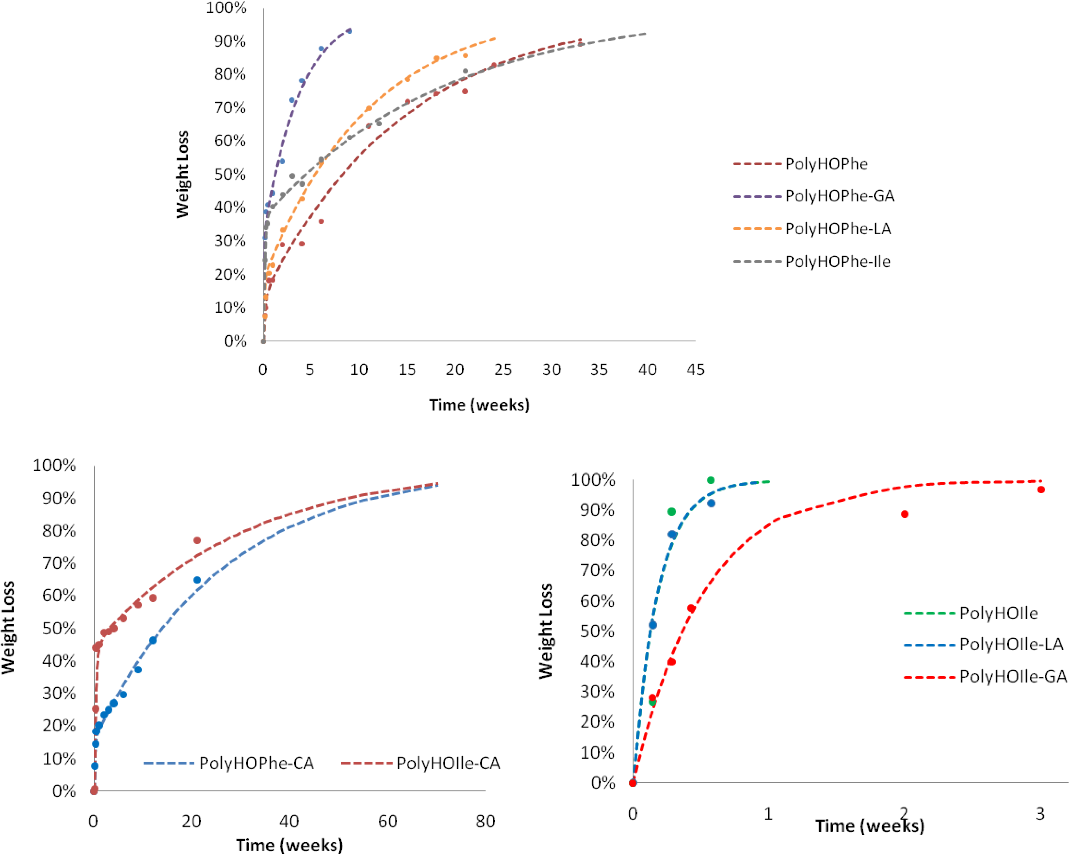
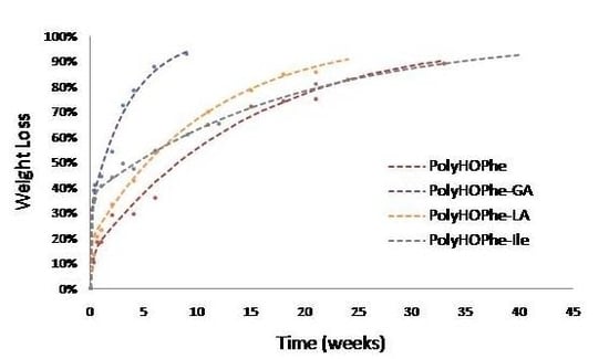
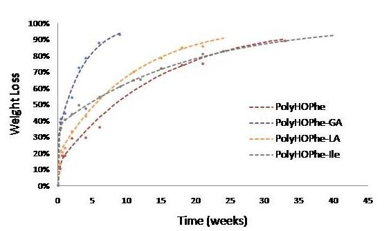
The biphasic reaction of copolymers of HOPhe and copolymers of HOIle is illustrated in
Figure 3. Copolymers of HOPhe with LA and HOIle have a half life of about three months in the burst phase whereas the insertion of GA reduces the half life time to less than a month. Indeed Panyam
et al. [
25] showed that the initial loss rate is found to be more rapid in PLGA polymers with high glycolic acid content. This is consistent with the more hydrophilic nature of the PLGA compared to lactide homo-polymers [
25].
Table 3.
The calculated rate constants (k1, k2, P1 and t(1/2) of each step) resulting from polymers degradation fitting using Equation 1.
Table 3.
The calculated rate constants (k1, k2, P1 and t(1/2) of each step) resulting from polymers degradation fitting using Equation 1.
| Polymer | k1(week−1) | P1 | k2 (week−1) | k1/k2 |
|---|
| t(0.5) h | t(0.5) weeks |
|---|
| PolyHOPhe | 4.75 | 13.45 | 0.0669 | 71 |
| 24.5 | 10.4 |
| Poly-HOPhe-CA | 6.12 | 15.95 | 0.0373 | 164 |
| 19.0 | 18.6 |
| PolyHOPhe-GA | 17.50 | 31.60 | 0.26 | 66.79 |
| 6.7 | 52.6 |
| PolyHOPhe-LA | 12 | 18.83 | 0.09 | 34.83 |
| 9.7 | 17.6 |
| PolyHOPhe-HOVal | 9.87 | 47.6 | 0.093 | 107 |
| 11.8 | 7.5 |
| PolyHOPhe-HOIle | 7.10 | 37.05 | 0.053 | 134 |
| 16.4 | 13.1 |
| PolyHOPhe-HOLeu | 8 | 22.38 | 0.0737 | 276 |
| 14.6 | 9.4 |
| PolyHOLeu | 2.605 | 44.4 | 0.073 | 36.3 |
| 44.8 | 9.5 |
| Poly-HOLeu-CA | 3.62 | 21.96 | 0.027 | 349 |
| 32.2 | 25.6 |
| PolyHOLeu-GA | 10.52 | 31.6 | 0.291 | 46.5 |
| 11.1 | 2.4 |
| PolyHOLeu-LA | 6.46 | 23.9 | 0.0719 | 89.8 |
| 18.0 | 9.6 |
| PolyHOLeu-HOVal | 5.06 | 33.78 | 0.028 | 316 |
| 23.0 | 24.7 |
| PolyHOLeu-HOIle | 5.08 | 26.9 | 0.0587 | 87.6 |
| 22.9 | 11.8 |
| PolyHOIle | 5.42 | – | – | – |
| 21.5 |
| PolyHOIle-CA | 2.91 | 44.62 | 0.0328 | 88.7 |
| 40.0 | 21.1 |
| PolyHOIle-GA | 1.91 | – | – | – |
| 60.9 |
| PolyHOIle-LA | 5.5 | – | – | – |
| 21.2 |
| PolyHOVal | 4.48 | – | – | – |
| 26.0 |
| PolyHOVal-CA | 2.91 | 66.47 | 0.0431 | 158 |
| 40.0 | 16.1 |
| PolyVal-GA | 3.97 | – | – | – |
| 29.3 |
| PolyHOVal-LA | 4.67 | – | – | – |
| 24.9 |
| PolyHOVal-HOIle | 5.10 | – | – | – |
| 22.8 |
Figure 3.
Hydrolysis of copolymers of HOPhe and copolymers of HOIle monitored by weight loss. The broken curves correspond to the theoretical rates whereas the points are the experimental values.
Figure 3.
Hydrolysis of copolymers of HOPhe and copolymers of HOIle monitored by weight loss. The broken curves correspond to the theoretical rates whereas the points are the experimental values.
This trend is inversed when evaluating copolymers of HOIle. The homopolymer and the copolymer with LA present a monophasic behavior and completely degrade in less than a week, whereas it takes three weeks for the HOIle-GA copolymer. These modulations are related to many aspects such as morphology of the sample, crystallinity, molecular weight of the polymer, and hydrophilicity, which may have significant impact on the degradation [
21,
24].
The effect of hydrophobicity on the degradation behavior of the polymers during the burst phase was also studied. Although the water contact angle gives an indication of the hydrophobicity of the polymer, no correlation was found between the water contact angle of the polymers and the weight loss constant, neither with Log P. Many factors are responsible for the contact angle of a polymer’s surface including surface contamination, heterogeneity of the surface structure, reorientation, mobility or roughness of the surface segment, swelling, and deformation [
26]. The properties of a polymer cast from a hydrophobic solvent (chloroform) on glass are different from the same polymer immersed into an aqueous medium. This might be the reason for the lack of correlation between degradation constants and contact angle results.
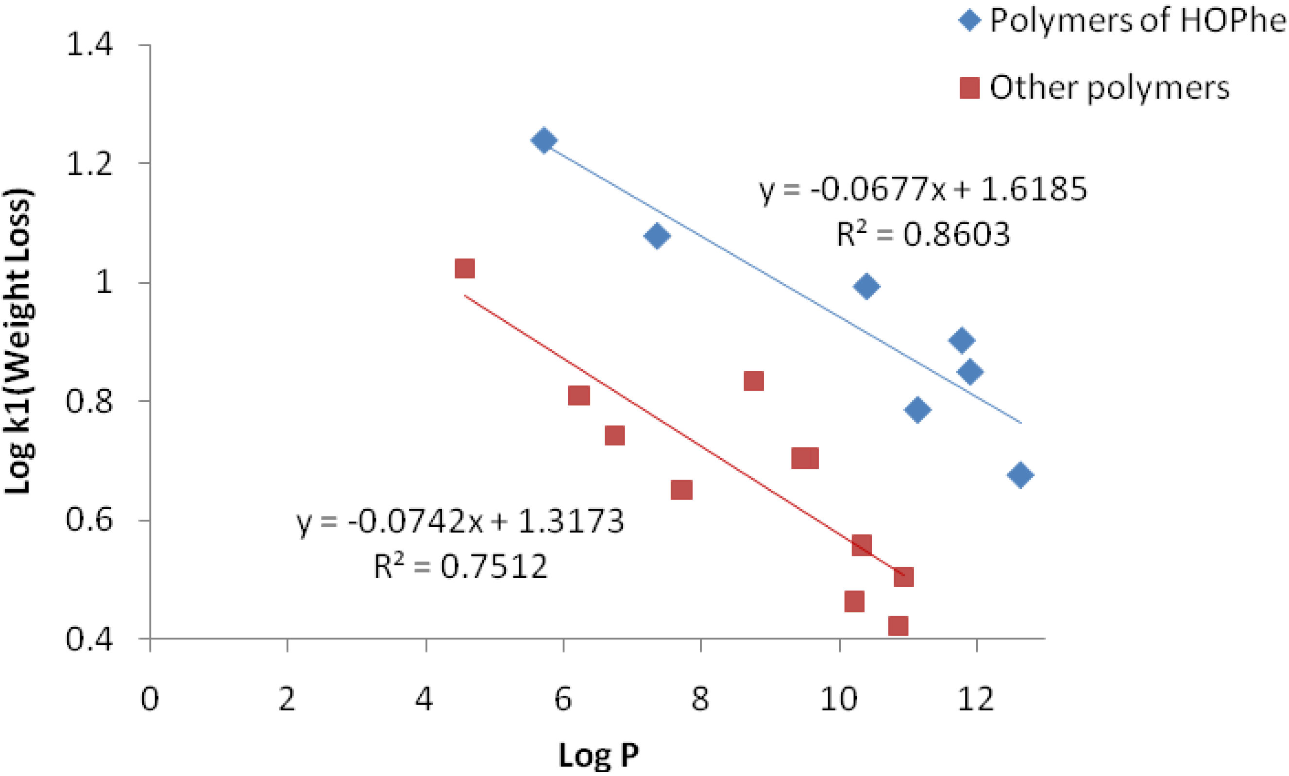
However, a linear correlation between the weight loss constant Log k
1 and the hydrophobicity Log P was found when the polymers were divided into two sets. The first set included homo and copolymers of HOPhe, while the second set involved homo and copolymers of HOVal, HOLeu and HOIle. Log P of the polymers was calculated by the ALOGPS 2.1 program, employing oligomers of 10 units for each polymer. The linear correlations are delineated in
Figure 4.
Figure 4.
Linear Correlation between Log k1 and Log P for the two sets of polymers.
Figure 4.
Linear Correlation between Log k1 and Log P for the two sets of polymers.
It can be concluded that the higher the hydrophobicity of the polymers, the slower the degradation rate. There is no linear dependence between the hydrophobicity (logP) and log k2, since the degradation of the inner part of the sample depends not only on the hydophobicity but also on the packing density of the matrix core.
Three polymers were not included in the linear correlation: PolyHOVal-LA, PolyHOIle-GA and PolyHOVal-GA since they are very hydrophilic and rapidly degrade to completion. The degradation rate of these polymers is not dependent on their hydrophobicity.
The difference between polymers of HOPhe and the other polymers can be explained by the fact that HOPhe is able to intercalate water molecules due to its spatial oriented aromatic ring, so that water molecules are more accessible for degradation during the burst stage. Thus, k1 of HOPhe copolymers are enhanced compared to other hydrophobic polymers.
Inspection of the second stage of the degradation revealed that copolymers of HOPhe and HOLeu are quite resistant to buffer medium and are slowly hydrolyzed during a period of several months (k
2 from 0.02 to 0.3 week
−1, t
1/2 = 3 to 25 weeks), whereas copolymers of HOIle and HOVal have a much shorter life time of several days to weeks (k
1 from 1 to 5 week
−1, t
1/2 = 22 to 60 hours). For copolymers of CA (
Table 1, compounds 20 and 23) their degradation time is extended (k
2 from 0.02 to 0.04 week
−1, t
1/2 = 16 to 21 weeks). However the degradation duration of copolymers of LA (
Table 1, compounds 12 to 15) is similar to the homopolymers.
From
Table 3, it is apparent that copolymers of CA are quite resistant to hydrolytic degradation and that in general these polymers discard only 70% (average) of their weight during five months. The inductive effect of the α-oxygen atom of the repeat unit in α-hydroxy polyesters enhances the reactivity of the ester carbonyl group and the acidity of the carboxylic end group, relative to the caproate ester structure [
27]. Subsequently, the polyesters of α-hydroxy acid appeared to be much more sensitive to hydrolytic reaction than their corresponding caproate copolymers.
2.3.3. GPC Analysis
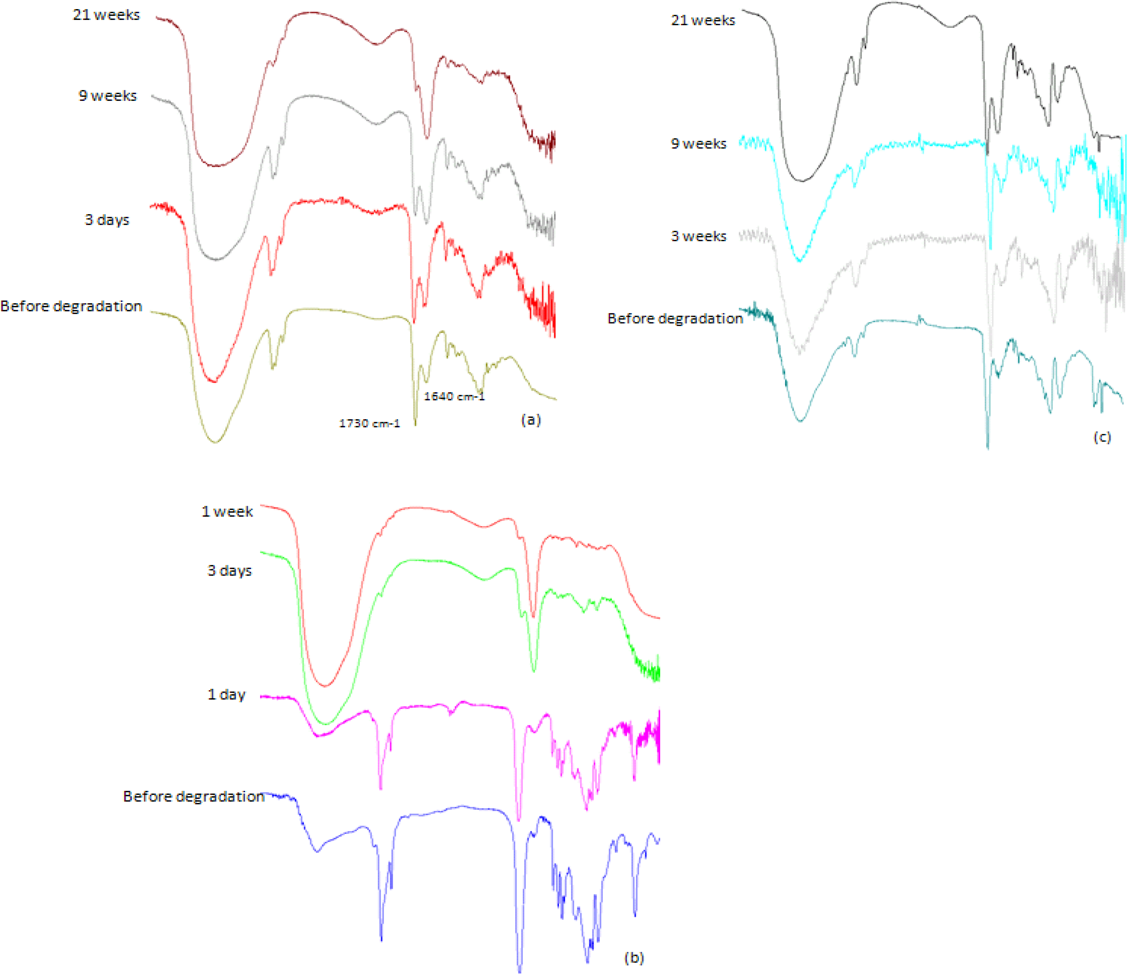
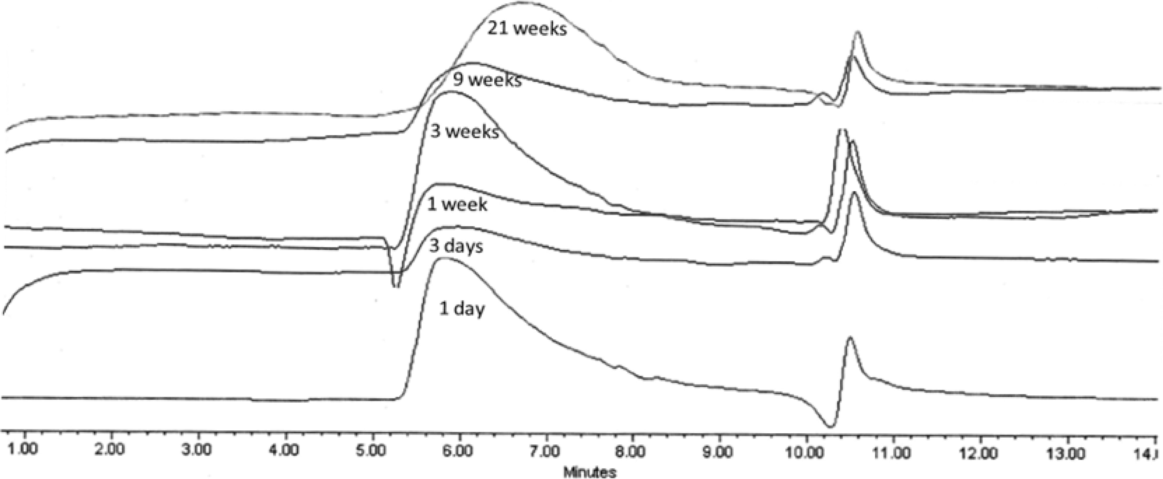
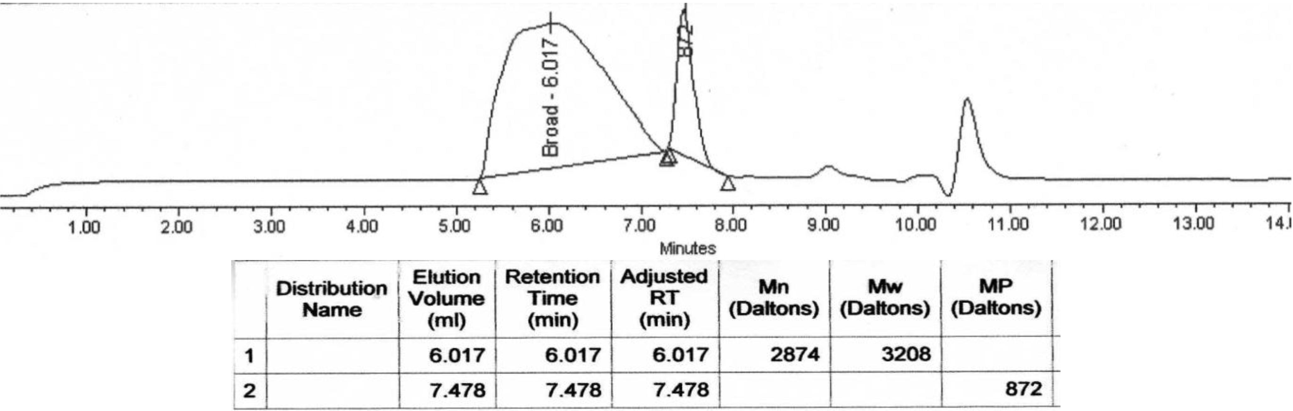
Molecular weight decrease was monitored by GPC analysis during the hydrolysis. Typical changes in the chromatograms during the course of the degradation process for PolyHOPhe-CA are illustrated in
Figure 6. Through the first week the chromatograms look alike and there is no significant change in the elution time of the sample. A slight increase in the molecular weight could be noticed due to the dissolution of small oligomers into the buffer solution [
28]. After three weeks of exposure to buffer, the chromatogram peak slowly moves to longer elution times. The molecular weight of the polymer starts to decrease.
Figure 6.
GPC chromatograms of PolyHOPhe-CA during the degradation.
Figure 6.
GPC chromatograms of PolyHOPhe-CA during the degradation.
The molecular weight decrease data was fitted (by a non linear regression) to a first order reaction rate equation composed of either one or two exponential terms as is presented in Equation 2. The data for some polymers showed a biphasic behavior regarding the molecular weight change while other polymers exhibited a monophasic behavior.
MW
t is the molecular weight of the residual polymer at time t. A
T is the initial molecular weight of the polymer and A
1 is the molecular weight of the polymer at the end of the first step. k
1 and k
2 are the rate constants of the first and second steps. The parameters of all polymers are summarized in
Table 4.
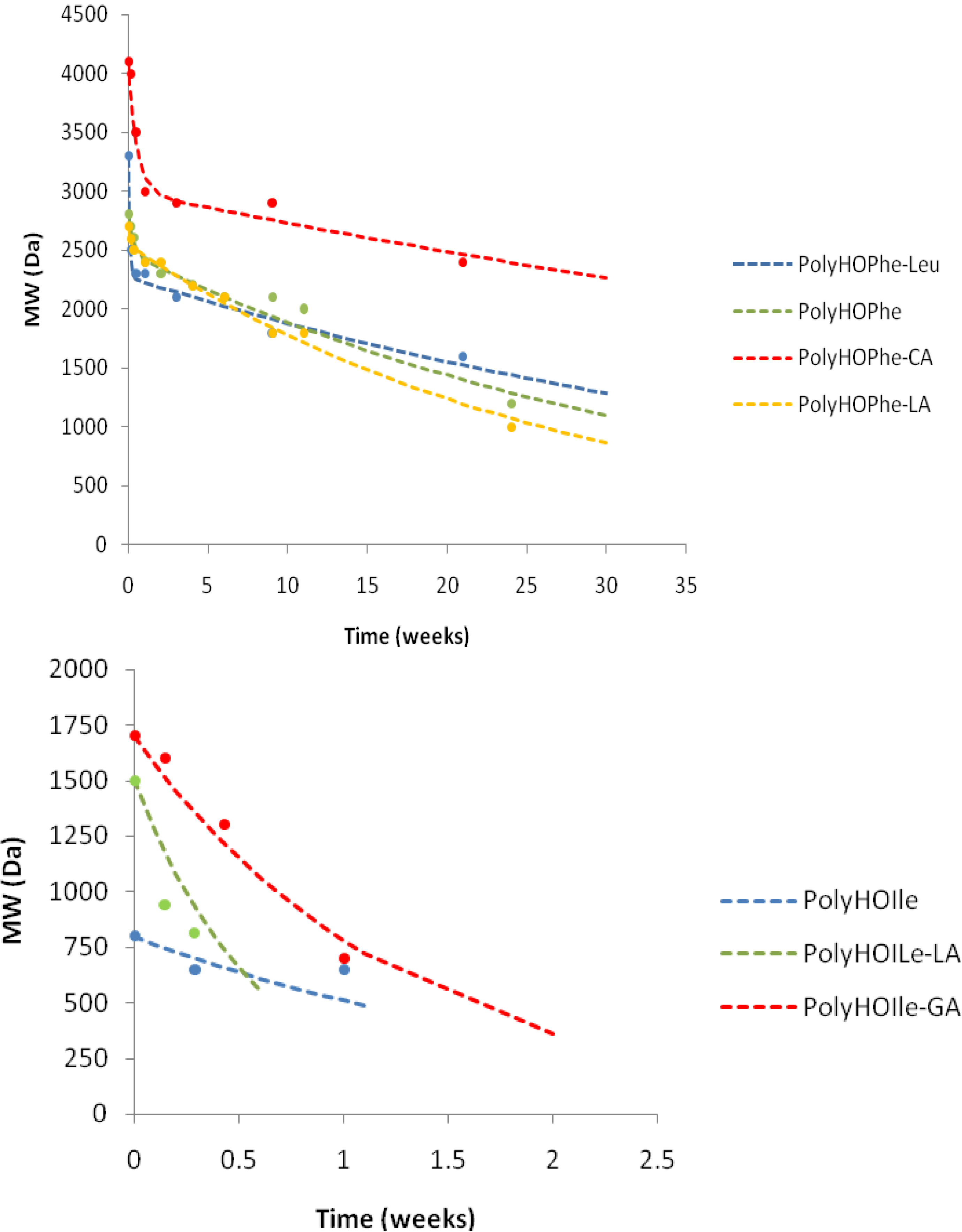
The Mw degradation curves are illustrated (in part) in
Figure 7.
Inspection of
Table 4 reveals that a significant number of polymers exhibited a biphasic behavior along the molecular weight decrease. The kinetic behavior of the molecular weight change was quite similar to that of the outlined weight loss, except for five polymers (PolyHOPhe-HOVal, PolyHOPhe-HOIle, PolyHOLeu-HOIle, PolyHOIle-CA, and PolyHOVal-CA). These polymers demonstrated a biphasic behavior in the weight loss experiment and monophasic behavior in their molecular weight decrease. Their k
1 values were low (from 0.01 to 0.07 week
−1, t
1/2 = 9 to 53 weeks), which is rather in the magnitude of k
2. Their molecular weight decrease was a slow, monophasic process. It is likely that their molecular weight remains constant during the first phase of weight loss (surface oligomers are hydrolyzed only), and the molecular weight decrease starts only towards the second phase of weight loss. For all other polymers, the magnitude of the rate constants for both processes was similar (weight loss and Mw decline), but the molecular weight decrease was slightly slower than the weight loss. The rate constants of the two processes are compared in
Table 5.
Table 4.
Calculated rate constants (k1, k2, A01 and t(1/2)) of molecular weight decrease emerging from fitting the experimental data to Equation 2. A01 is the percentage of the molecular weight decrease at the end of the first step of degradation (A01 = (AT − A1) ÷ AT × 100).
Table 4.
Calculated rate constants (k1, k2, A01 and t(1/2)) of molecular weight decrease emerging from fitting the experimental data to Equation 2. A01 is the percentage of the molecular weight decrease at the end of the first step of degradation (A01 = (AT − A1) ÷ AT × 100).
| Polymer | k1(week−1) | A01 | k2(week−1) | k1/k2 |
|---|
| t(0.5)h | t(0.5)weeks |
|---|
| PolyHOPhe | 3.03 | 11.2 | 0.027 | 105 |
| 38.04 | 25.6 |
| PolyHOPhe-CA | 1.87 | 27 | 0.0094 | 198 |
| 62.2 | 73.2 |
| PolyHOPhe-GA | 1.44 | 28.4 | 0.018 | 80 |
| 80.85 | 38.5 |
| PolyHOPhe-LA | 8.54 | 5.6 | 0.036 | 237 |
| 13.6 | 19.25 |
| PolyHOPhe-Val | 0.0738 | – | – | – |
| 9.4 weeks |
| PolyHOPhe-Ile | 0.0176 | – | – | – |
| 39.4 weeks |
| PolyHOPhe-Leu | 10.39 | 31 | 0.019 | 546 |
| 11.2 | 36.5 |
| PolyHOLeu | 8.157 | 31 | 0.059 | 138 |
| 14.2 | 11.7 |
| PolyHOLeu-CA | 1.26 | 39 | 0.0074 | 170.2 |
| 92.4 | 93.6 |
| PolyHOLeu-GA | 0.786 | 32.8 | 0.0113 | 69 |
| 148 | 61.3 |
| PolyHOLeu-LA | 8.085 | 9.4 | 0.0462 | 89.8 |
| 14.4 | 15 |
| PolyHOLeu-Val | 4.72 | 23 | 0.020 | 236 |
| 24.6 | 34.6 |
| PolyHOLeu-Ile | 0.0738 | – | – | – |
| 9.4 weeks |
| PolyHOIle | 0.448 | – | – | – |
| 260 |
| PolyHOIle-CA | 0.045 | – | – | – |
| 15.4 weeks |
| PolyHOIle-GA | 0.781 | – | – | – |
| 149 |
| PolyHOIle-LA | 1.656 | – | – | – |
| 70.3 |
| PolyHOVal | 0.395 | – | – | – |
| 294 |
| PolyHOVal-CA | 0.0131 | – | – | – |
| 53.0 weeks |
| PolyHOVal-GA | 2.40 | – | – | – |
| 48.5 |
| PolyHOVal-LA | 1.145 | – | – | – |
| 119 |
| PolyHOVal-Ile | 0.327 | – | – | – |
| 356 |
Figure 7.
Kinetic pattern of molecular weight decrease during hydrolysis.
Figure 7.
Kinetic pattern of molecular weight decrease during hydrolysis.
During the burst stage in the weight loss course the main process seems to be the dissolution of small oligomers present in the polymer mass, which does not result in molecular weight decrease. This process can even potentially yield an increase in the molecular weight. During the second stage of weight loss, the polymer is cleaved but the weight loss remains faster than the change in molecular weight as shown in
Table 5.
Table 5.
Comparison between rate constants of weight loss and molecular weight change experiments.
Table 5.
Comparison between rate constants of weight loss and molecular weight change experiments.
| Weight Loss | MW Decrease |
|---|
| k1 | 1.9 to 17.5 week−1 | 0.3 to 10 week−1 |
| k2 | 0.02 to 0.3 week−1 | 0.007 to 0.06 week−1 |
| t1/2(1) | 6.7 to 60 hours | 11 to 356 hours |
| t1/2(2) | 2.6 to 26 weeks | 11 to 93 weeks |
Generally, it was established that polyesters containing either HOVal or HOIle degraded to oligomers of less than 1000 Da within a few days (k1 = 0.4 to 2.4 week−1), independently of the initial molecular weight. This fast decrease is parallel to their rapid weight loss, which is monophasic. On the other hand, polyesters containing HOLeu and HOPhe exhibited significantly slower decreases in molecular weight in accordance with their weight loss behavior. The difference between these two groups might be due to the spatial orientation of the aliphatic chains/ring along the polymer. Copolymers of CA show a decrease in Mw during the first two or three weeks to attain a molecular weight of 2000–3000 Da, remaining at a constant value for the leftover period of the degradation experiment. The insertion of GA in the polymers accelerates the hydrolytic rate whereas LA does not significantly affect molecular weight decrease (or similarly, the weight loss).
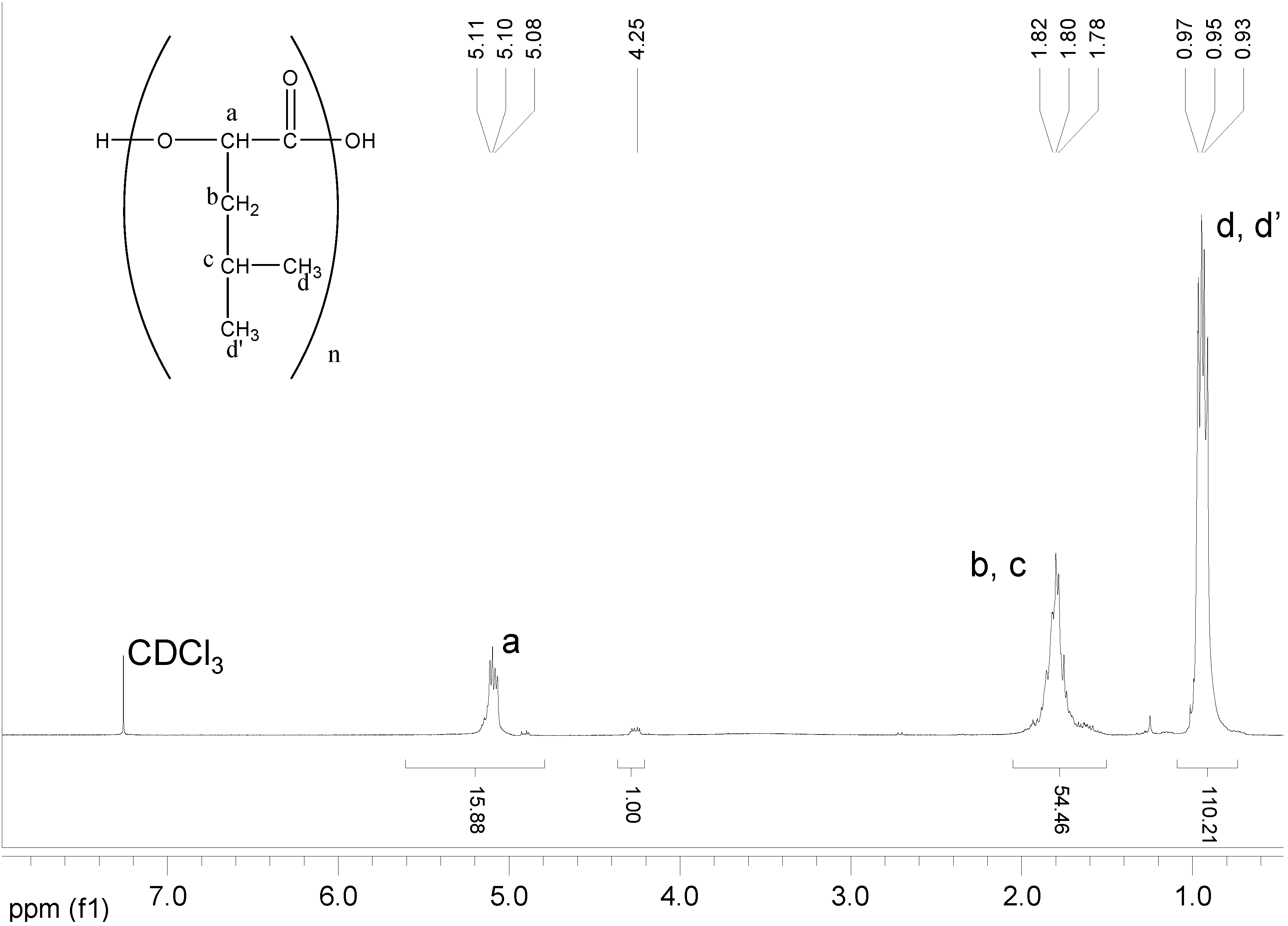
2.3.4. NMR Analysis
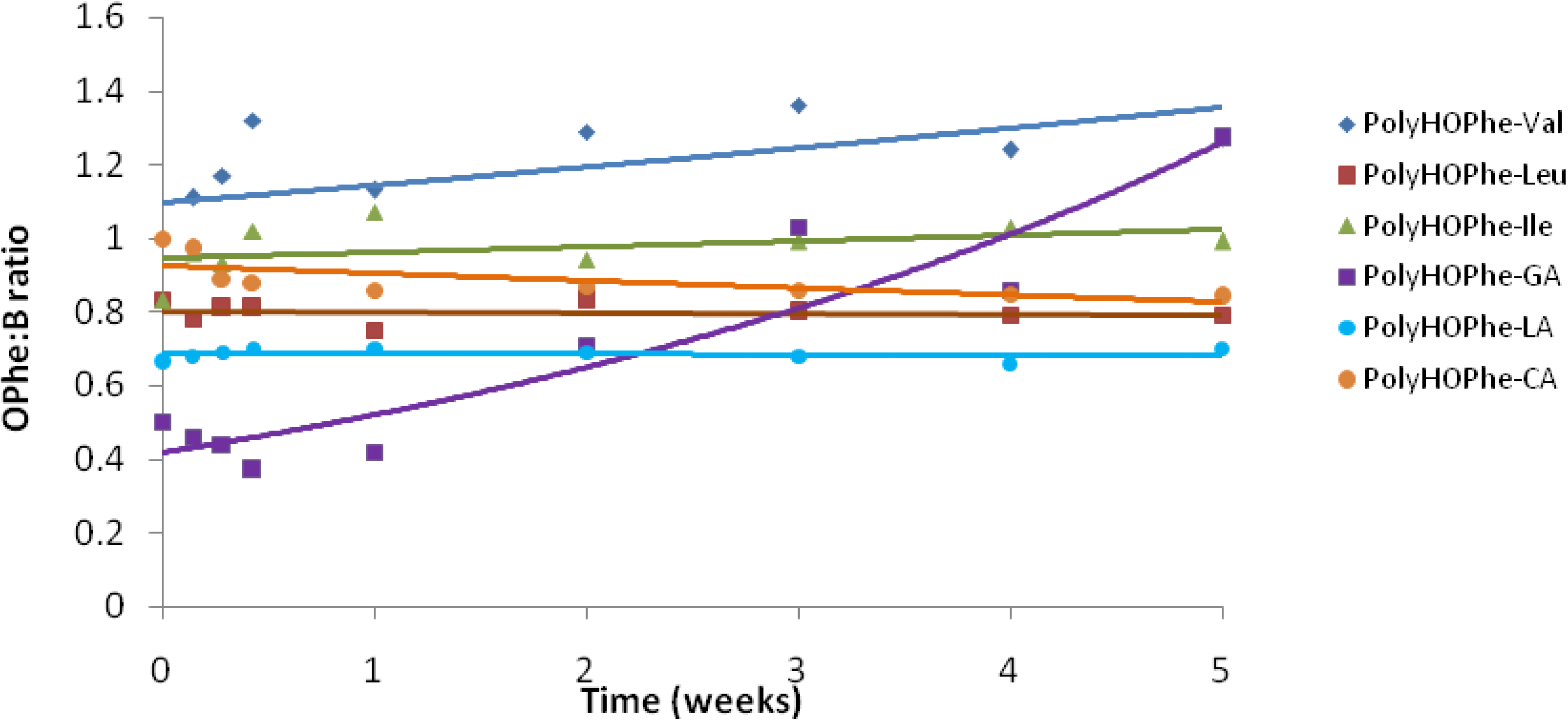
Copolymers of HOPhe were monitored by NMR in order to determine the ratio between the two units in the polymer during degradation. For each copolymer, two peaks were selected in the NMR spectrum. One was assigned to unit A (-OPhe-) and the other was assigned to B (
Table 6). At each time point, the ratio between A (-OPhe-) and B was calculated and the results are plotted in
Figure 8.
It is apparent that for PolyHOPhe-Leu and PolyHOPhe-LA, the two components (-OPhe-) and B(-OLeu and -OLA) were released at the same rate (horizontal lines) and there is no change in the polymer composition during the degradation. On the other hand, the ratio between HOPhe and GA growed during the degradation process, meaning that GA was evacuated faster from the polymer than HOPhe. This is also the case with PolyHOPhe-Val and PolyHOPhe-Ile, although the change was less pronounced. An inverse trend can be observed for PolyHOPhe-CA, in which the HOPhe unit was released faster to the buffer medium than the CA one.
It is conceivable to assume that a unit that is cleared faster from the polyester is more sensitive to hydrolytic degradation due to its hydrophilicity (GA) or side chain orientation (HOVal and HOIle). CA is less susceptible to hydrolysis than HOPhe as a result of the α-hydroxy acid effect explained above. The change in polymer composition affects the profile of the hydrolysis.
Table 6.
NMR peaks corresponding to unit A (-OPhe-) and B in the copolymers PolyHOPhe-B and their initial ratios.
Table 6.
NMR peaks corresponding to unit A (-OPhe-) and B in the copolymers PolyHOPhe-B and their initial ratios.
| Copolymer | Chemical shift of Peak A (HOPhe, ppm) | Chemical shift of Peak B (ppm) | A:B at t = 0 |
|---|
| PolyHOPhe-Ile | 7.26 (5 aromatic protons) | 0.92 (6 methyl protons) | 5:6 |
| PolyHOPhe-Leu | 7.26 (5 aromatic protons) | 0.93 (6 methyl protons) | 5:6 |
| PolyHOPhe-Val | 7.26 (5 aromatic protons) | 0.85 (6 methyl protons) | 5:6 |
| PolyHOPhe-LA | 3.18 (2 CH2 protons) | 1.52 (3 methyl protons) | 2:3 |
| PolyHOPhe-GA | 5.32 (1 CH proton) | 4.72 (2 CH2 protons) | 1:2 |
| PolyHOPhe-CA | 3.18 (2 CH2 protons) | 2.29 (2 CH2 protons) | 1:1 |
Figure 8.
Composition of the HOPhe-B copolymers during degradation as been derived from NMR data.
Figure 8.
Composition of the HOPhe-B copolymers during degradation as been derived from NMR data.


