
Diffusion-Enhanced Förster Resonance Energy Transfer in Flexible Peptides: From the Haas-Steinberg Partial Differential Equation to a Closed Analytical Expression

Abstract
:
1. Introduction
Introduction to the Haas-Steinberg Equation
2. Materials and Methods
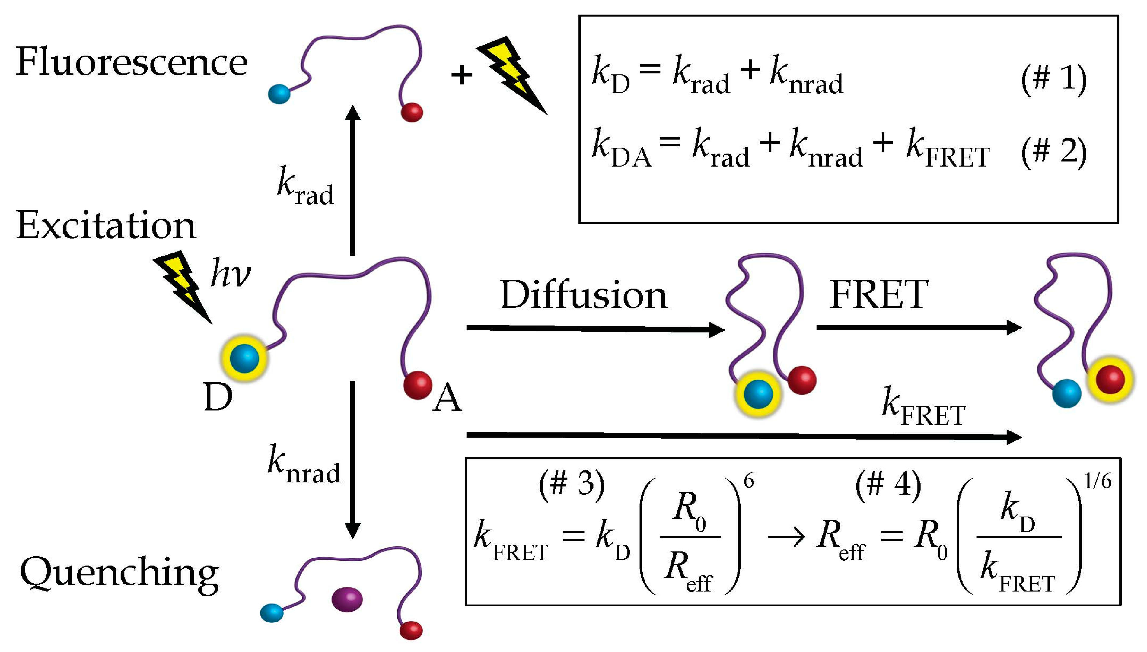
2.1. The HSE
2.2. Steinberg’s Derivation
3. Results
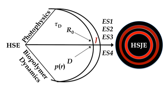
3.1. Ideas and Concepts
3.2. The Equivalence Statements
3.2.1. The First Equivalence Statement: Variation of the Distance Distribution
Equivalence Statement 1 (ES1, Text)
- 1.
- Why do we demand that rL(1) = rL(2)? Why can ES1 not be applied if the left-integration limit differs in both sets?
- 2.
- Is ES1 valid for any distance distribution equation or model? Or is it only valid for “well-behaved” models?
3.2.2. The Second Equivalence Statement: Variation of the Donor Lifetime
Equivalence Statement 2 (ES2, Text)
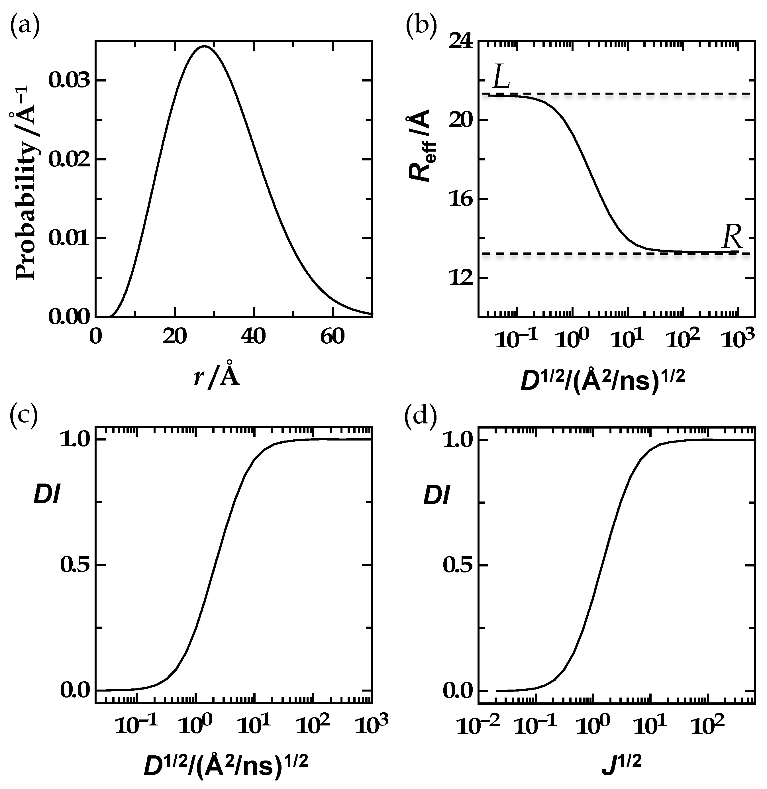
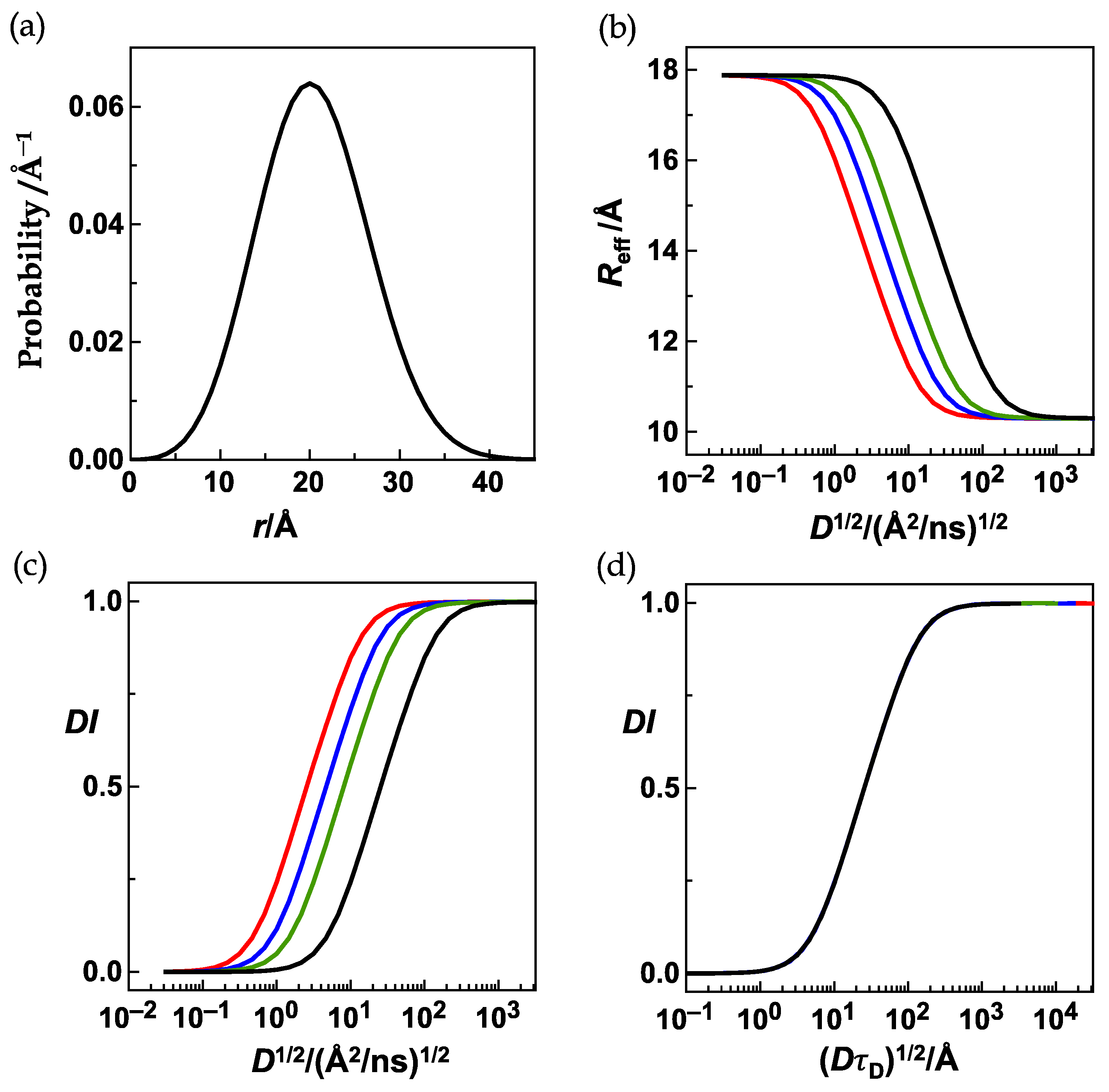
3.2.3. The Third Equivalence Statement: Variation of the Förster Radius and Left-Integration Limit
Equivalence Statement 3 (ES3, Text)
3.2.4. The Fourth Equivalence Statement
Equivalence Statement 4 (ES4, Text)
3.3. The Grid
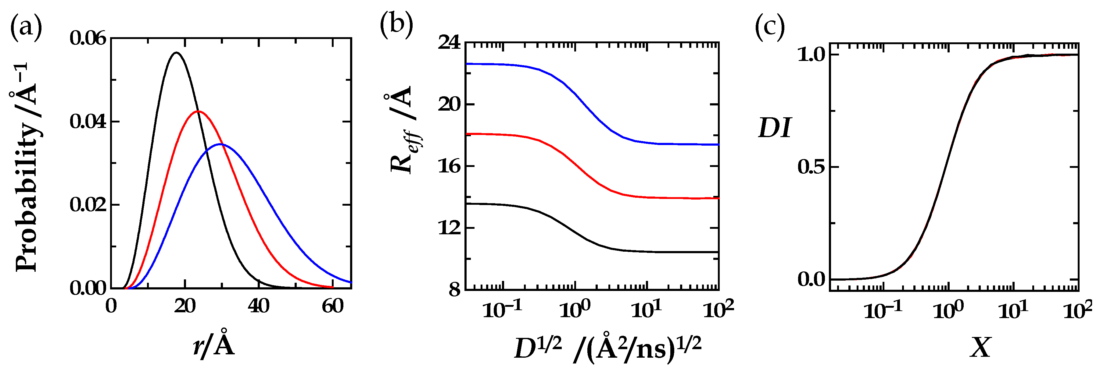
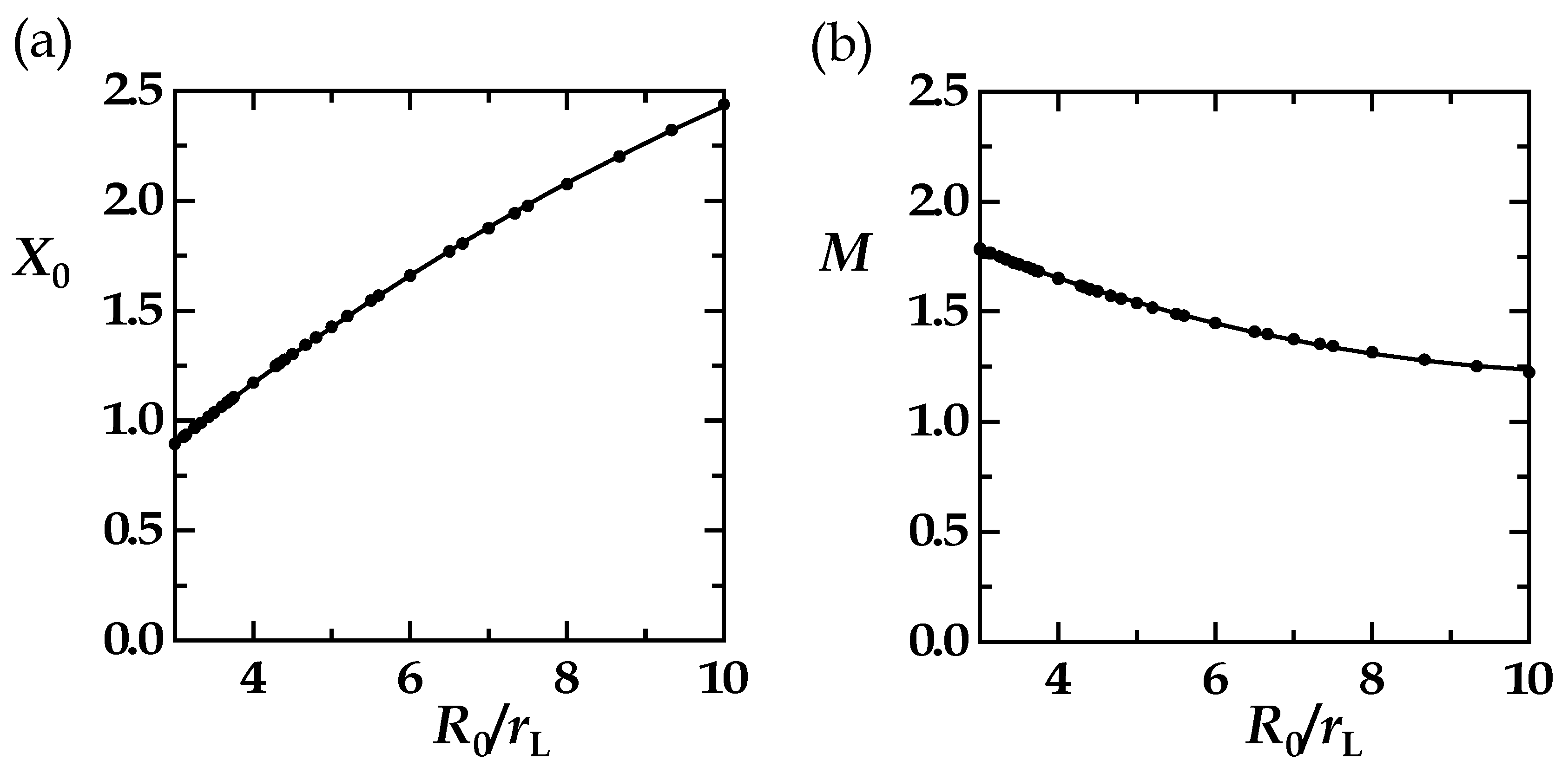
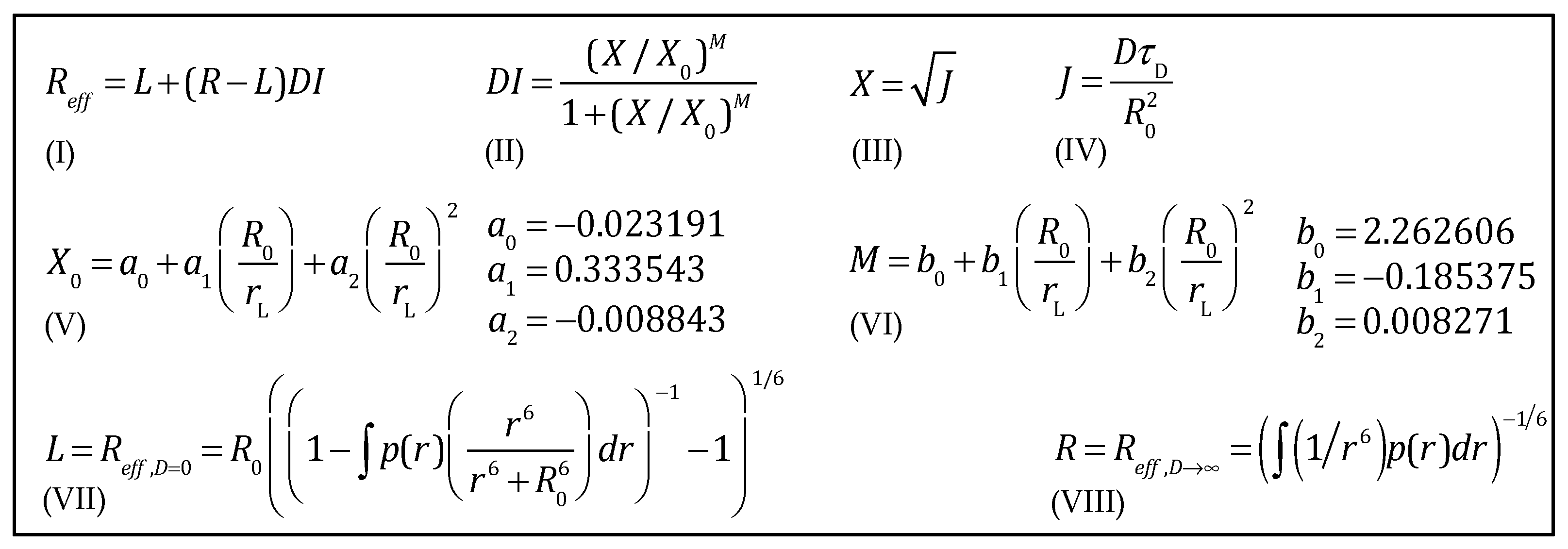
3.4. The HSJE
4. Discussion
5. Conclusions
Supplementary Materials
Author Contributions
Funding
Institutional Review Board Statement
Informed Consent Statement
Data Availability Statement
Acknowledgments
Conflicts of Interest
References
- Ingargiola, A.; Weiss, S.; Lerner, E. Monte Carlo Diffusion-Enhanced Photon Inference: Distance Distributions and Conformational Dynamics in Single-Molecule FRET. J. Phys. Chem. B 2018, 122, 11598–11615. [Google Scholar] [CrossRef] [PubMed] [Green Version]
- Förster, T. Zwischenmolekulare Energiewanderung und Fluoreszenz. Ann. Phys. 1948, 2, 55–75. [Google Scholar] [CrossRef]
- Haas, E.; Katchalski-Katzir, E.; Steinberg, I.Z. Brownian Motion of the Ends of Oligopeptides Chains in Solution as Estimated by Energy Transfer between the Chain Ends. Biopolymers 1978, 17, 11–31. [Google Scholar] [CrossRef]
- Stryer, L.; Thomas, D.D.; Meares, C.F. Diffusion-Enhanced Fluorescence Energy Transfer. Annu. Rev. Biophys. Bioeng. 1982, 11, 203–222. [Google Scholar] [CrossRef] [PubMed]
- Beechem, J.M.; Haas, E. Simultaneous Determination of Intramolecular Distance Distributions and Conformational Dynamics by Global Analysis of Energy Transfer Measurements. Biophys. J. 1989, 55, 1225–1236. [Google Scholar] [CrossRef] [Green Version]
- Lakowicz, J.R.; Kusba, J.; Gryczynski, I.; Wiczk, W.; Szmacinski, H.; Johnson, M.L. End-to-End Diffusion and Distance Distributions of Flexible Donor-Acceptor Systems Observed by Intramolecular Energy-Transfer and Frequency-Domain Fluorometry—Enhanced Resolution by Global Analysis of Externally Quenched and Nonquenched Samples. J. Phys. Chem. B 1991, 95, 9654–9660. [Google Scholar] [CrossRef]
- Maliwal, B.P.; Kusba, J.; Wiczk, W.; Johnson, M.L.; Lakowicz, J.R. End-to-End Diffusion Coefficients and Distance Distributions from Fluorescence Energy Transfer Measurements: Enhanced Resolution by Using Multiple Acceptors with Different Förster Distances. Biophys. Chem. 1993, 46, 273–281. [Google Scholar] [CrossRef]
- Steinberg, I.Z. Brownian Motion of the End-to-End Distance in Oligopeptide Molecules: Numerical Solution of the Diffusion Equations as Coupled First Order Linear Differential Equations. J. Theor. Biol. 1994, 166, 173–187. [Google Scholar] [CrossRef] [PubMed]
- Gryczynski, I.; Lakowicz, J.R.; Kusba, J. End-to-End Diffusion Coefficients and Distance Distributions from Fluorescence Energy Transfer Measurements: Enhanced Resolution by Using Multiple Donors with Different Lifetimes. J. Fluoresc 1995, 5, 195–203. [Google Scholar] [CrossRef]
- Möglich, A.; Joder, K.; Kiefhaber, T. End-to-End Distance Distributions and Intrachain Diffusion Constants in Unfolded Polypeptide Chains Indicate Intramolecular Hydrogen Bond Formation. Proc. Natl. Acad. Sci. USA 2006, 103, 12394–12399. [Google Scholar] [CrossRef] [Green Version]
- Grupi, A.; Haas, E. Segmental Conformational Disorder and Dynamics in the Intrinsically Disordered Protein Alpha-Synuclein and Its Chain Length Dependence. J. Mol. Biol. 2011, 405, 1267–1283. [Google Scholar] [CrossRef]
- Jacob, M.H.; Dsouza, R.N.; Ghosh, I.; Norouzy, A.; Schwarzlose, T.; Nau, W.M. Diffusion-Enhanced Forster Resonance Energy Transfer and the Effects of External Quenchers and the Donor Quantum Yield. J. Phys. Chem. B 2013, 117, 185–198. [Google Scholar] [CrossRef] [PubMed]
- Jacob, M.H.; D’Souza, R.N.; Schwarzlose, T.; Wang, X.; Huang, F.; Haas, E.; Nau, W.M. Method-Unifying View of Loop-Formation Kinetics in Peptide and Protein Folding. J. Phys. Chem. B 2018, 122, 4445–4456. [Google Scholar] [CrossRef] [PubMed]
- Jacob, M.H.; Ghosh, I.; D’Souza, R.N.; Nau, W.M. Two Orders of Magnitude Variation of Diffusion-Enhanced Förster Resonance Energy Transfer in Polypeptide Chains. Polymers 2018, 10, 1079. [Google Scholar] [CrossRef] [Green Version]
- Lerner, E.; Orevi, T.; Ben Ishay, E.; Amir, D.; Haas, E. Kinetics of Fast Changing Intramolecular Distance Distributions Obtained by Combined Analysis of Fret Efficiency Kinetics and Time-Resolved Fret Equilibrium Measurements. Biophys. J. 2014, 106, 667–676. [Google Scholar] [CrossRef] [PubMed] [Green Version]
- May, V.; Kühn, O. Charge and Energy Transfer Dynamics in Molecular Systems; Wiley-VCH: Berlin, Germany, 2000. [Google Scholar]
- Sahoo, H.; Roccatano, D.; Zacharias, M.; Nau, W.M. Distance Distributions of Short Polypeptides Recovered by Fluorescence Resonance Energy Transfer in the 10 Å Domain. J. Am. Chem. Soc. 2006, 128, 8118–8119. [Google Scholar] [CrossRef]
- Jacob, M.H.; Nau, W.M. Short-Distance FRET Applied to the Polypeptide Chain. In Folding, Misfolding and Nonfolding of Peptides and Small Proteins; Schweitzer-Stenner, R., Ed.; John Wiley & Sons: Hoboken, NJ, USA, 2011. [Google Scholar]
- Casier, R.; Duhamel, J. Pyrene Excimer Fluorescence as a Direct and Easy Experimental Means to Characterize the Length Scale and Internal Dynamics of Polypeptide Foldons. Macromolecules 2018, 51, 3450–3457. [Google Scholar] [CrossRef]
- Orevi, T.; Lerner, E.; Rahamim, G.; Amir, D.; Haas, E. Ensemble and Single-Molecule Detected Time-Resolved Fret Methods in Studies of Protein Conformations and Dynamics. Methods. Mol. Biol. 2014, 1076, 113–169. [Google Scholar]
- Stryer, L. Fluorescence Energy Transfer as a Spectroscopic Ruler. Ann. Rev. Biochem. 1978, 47, 819–846. [Google Scholar] [CrossRef]
- Duhamel, J.; Yekta, A.; Winnik, M.A.; Jao, T.C.; Mishra, M.K.; Rubin, I.D. A Blob Model to Study Polymer Chain Dynamics in Solution. J. Phys. Chem. 1993, 97, 13708–13712. [Google Scholar] [CrossRef]
- Weiss, S. Measuring Conformational Dynamics of Biomolecules by Single Molecule Fluorescence Spectroscopy. Nat. Struct. Biol. 2000, 7, 724–729. [Google Scholar] [CrossRef] [PubMed]
- Broos, J.; Pas, H.H.; Robillard, G.T. The Smallest Resonance Energy Transfer Acceptor for Tryptophan. J. Am. Chem. Soc. 2002, 124, 6812–6813. [Google Scholar] [CrossRef] [Green Version]
- Hudgins, R.R.; Huang, F.; Gramlich, G.; Nau, W.M. A Fluorescence-Based Method for Direct Measurement of Submicrosecond Intramolecular Contact Formation in Biopolymers: An Exploratory Study with Polypeptides. J. Am. Chem. Soc. 2002, 124, 556–564. [Google Scholar] [CrossRef]
- Duhamel, J.; Kanagalingam, S.; O’Brien, T.J.; Ingratta, M.W. Side-Chain Dynamics of an Alpha-Helical Polypeptide Monitored by Fluorescence. J. Am. Chem. Soc. 2003, 125, 12810–12822. [Google Scholar] [CrossRef] [PubMed]
- Nau, W.M.; Huang, F.; Wang, X.J.; Bakirci, H.; Gramlich, G.; Marquez, C. Exploiting Long-Lived Molecular Fluorescence. Chimia 2003, 57, 161–167. [Google Scholar] [CrossRef]
- Schuler, B.; Lipman, E.A.; Steinbach, P.J.; Kumke, M.; Eaton, W.A. Polyproline and the “Spectroscopic Ruler” Revisited with Single- Molecule Fluorescence. Proc. Natl. Acad. Sci. USA 2005, 102, 2754–2759. [Google Scholar] [CrossRef] [PubMed] [Green Version]
- Duhamel, J. Polymer Chain Dynamics in Solution Probed with a Fluorescence Blob Model. Acc. Chem. Res. 2006, 39, 953–960. [Google Scholar] [CrossRef] [PubMed]
- Sahoo, H.; Nau, W.M. Phosphorylation-Induced Conformational Changes in Short Peptides Probed by Fluorescence Resonance Energy Transfer in the 10-Å Domain. ChemBioChem 2007, 8, 567–573. [Google Scholar] [CrossRef]
- Sahoo, H.; Roccatano, D.; Hennig, A.; Nau, W.M. A 10-a Spectroscopic Ruler Applied to Short Polyprolines. J. Am. Chem. Soc. 2007, 129, 9762–9772. [Google Scholar] [CrossRef]
- Schuler, B. Application of Single Molecule Forster Resonance Energy Transfer to Protein Folding. Methods Mol. Biol. 2007, 350, 115–138. [Google Scholar]
- Glasscock, J.M.; Zhu, Y.J.; Chowdhury, P.; Tang, J.; Gai, F. Using an Amino Acid Fluorescence Resonance Energy Transfer Pair to Probe Protein Unfolding: Application to the Villin Headpiece Subdomain and the Lysm Domain. Biochemistry 2008, 47, 11070–11076. [Google Scholar] [CrossRef] [PubMed] [Green Version]
- Haas, E. Protein Folding Handbook; Buchner, K., Ed.; John Wiley & Sons: Hoboken, NJ, USA, 2008. [Google Scholar]
- Ingratta, M.; Duhamel, J. Effect of Side-Chain Length on the Side-Chain Dynamics of Alpha-Helical Poly(L-Glutamic Acid) as Probed by a Fluorescence Blob Model. J. Phys. Chem. B 2008, 112, 9209–9218. [Google Scholar] [CrossRef] [PubMed]
- Ingratta, M.; Hollinger, J.; Duhamel, J. A Case for Using Randomly Labeled Polymers to Study Long-Range Polymer Chain Dynamics by Fluorescence. J. Am. Chem. Soc. 2008, 130, 9420–9428. [Google Scholar] [CrossRef] [PubMed]
- Khan, Y.R.; Dykstra, T.E.; Scholes, G.D. Exploring the Förster Limit in a Small FRET Pair. Chem. Phys. Lett. 2008, 461, 305–309. [Google Scholar] [CrossRef]
- Orevi, T.; Ishay, E.B.; Pirchi, M.; Jacob, M.H.; Amir, D.; Haas, E. Early Closure of a Long Loop in the Refolding of Adenylate Kinase: A Possible Key Role of Non-Local Interactions in the Initial Folding Steps. J. Mol. Biol. 2009, 385, 1230–1242. [Google Scholar] [CrossRef]
- Chen, S.; Duhamel, J.; Winnik, M.A. Probing End-to-End Cyclization Beyond Willemski and Fixman. J. Phys. Chem. B 2011, 115, 3289–3302. [Google Scholar] [CrossRef]
- Grupi, A.; Haas, E. Time-Resolved Fret Detection of Subtle Temperature-Induced Conformational Biases in Ensembles of Alpha-Synuclein Molecules. J. Mol. Biol. 2011, 411, 234–247. [Google Scholar] [CrossRef]
- Ben Ishay, E.; Rahamim, G.; Orevi, T.; Hazan, G.; Amir, D.; Haas, E. Fast Subdomain Folding Prior to the Global Refolding Transition of E. coli Adenylate Kinase: A Double Kinetics Study. J. Mol. Biol. 2012, 423, 613–623. [Google Scholar] [CrossRef]
- Fowler, M.A.; Duhamel, J.; Bahun, G.J.; Adronov, A.; Zaragoza-Galan, G.; Rivera, E. Studying Pyrene-Labeled Macromolecules with the Model-Free Analysis. J. Phys. Chem. B 2012, 116, 14689–14699. [Google Scholar] [CrossRef]
- Chen, S.; Duhamel, J. Probing the Hydrophobic Interactions of a Series of Pyrene End-Labeled Poly(Ethylene Oxide)S in Aqueous Solution Using Time-Resolved Fluorescence. Langmuir 2013, 29, 2821–2834. [Google Scholar] [CrossRef]
- Lerner, E.; Hilzenrat, G.; Amir, D.; Tauber, E.; Garini, Y.; Haas, E. Preparation of Homogeneous Samples of Double-Labelled Protein Suitable for Single-Molecule Fret Measurements. Anal. Bioanal. Chem. 2013, 405, 5983–5991. [Google Scholar] [CrossRef] [PubMed]
- Orevi, T.; Rahamim, G.; Hazan, G.; Amir, D.; Haas, E. The Loop Hypothesis: Contribution of Early Formed Specific Non-Local Interactions to the Determination of Protein Folding Pathways. Biophys. Rev. 2013, 5, 85–98. [Google Scholar] [CrossRef] [PubMed] [Green Version]
- Duhamel, J. Global Analysis of Fluorescence Decays to Probe the Internal Dynamics of Fluorescently Labeled Macromolecules. Langmuir 2014, 30, 2307–2324. [Google Scholar] [CrossRef] [PubMed]
- Orevi, T.; Ben Ishay, E.; Gershanov, S.L.; Dalak, M.B.; Amir, D.; Haas, E. Fast Closure of N-Terminal Long Loops but Slow Formation of Beta Strands Precedes the Folding Transition State of Escherichia coli Adenylate Kinase. Biochemistry 2014, 53, 3169–3178. [Google Scholar] [CrossRef]
- Zaragoza-Galán, G.; Fowler, M.; Rein, R.; Solladié, N.; Duhamel, J.; Rivera, E. Fluorescence Resonance Energy Transfer in Partially and Fully Labeled Pyrene Dendronized Porphyrins Studied with Model Free Analysis. J. Phys. Chem. C 2014, 118, 8280–8294. [Google Scholar] [CrossRef]
- Norouzy, A.; Assaf, K.I.; Zhang, S.; Jacob, M.H.; Nau, W.M. Coulomb Repulsion in Short Polypeptides. J. Phys. Chem. B 2015, 119, 33–43. [Google Scholar] [CrossRef]
- Rahamim, G.; Chemerovski-Glikman, M.; Rahimipour, S.; Amir, D.; Haas, E. Resolution of Two Sub-Populations of Conformers and Their Individual Dynamics by Time Resolved Ensemble Level Fret Measurements. PLoS ONE 2015, 10, e0143732. [Google Scholar] [CrossRef] [PubMed] [Green Version]
- Toptygin, D. Effect of Diffusion on Resonance Energy Transfer Rate Distributions: Implications for Distance Measurements. J. Phys. Chem. B 2015, 119, 12603–12622. [Google Scholar] [CrossRef]
- Duhamel, J. Long Range Polymer Chain Dynamics Studied by Fluorescence Quenching. Macromolecules 2016, 49, 6149–6162. [Google Scholar]
- Orevi, T.; Rahamim, G.; Amir, D.; Kathuria, S.; Bilsel, O.; Matthews, C.R.; Haas, E. Sequential Closure of Loop Structures Forms the Folding Nucleus During the Refolding Transition of the Escherichia coli Adenylate Kinase Molecule. Biochemistry 2016, 55, 79–91. [Google Scholar] [CrossRef]
- Peulen, T.O.; Opanasyuk, O.; Seidel, C.A.M. Combining Graphical and Analytical Methods with Molecular Simulations to Analyze Time-Resolved FRET Measurements of Labeled Macromolecules Accurately. J. Phys. Chem. B 2017, 121, 8211–8241. [Google Scholar] [CrossRef] [PubMed] [Green Version]
- Song, J.; Gomes, G.N.; Shi, T.; Gradinaru, C.C.; Chan, H.S. Conformational Heterogeneity and Fret Data Interpretation for Dimensions of Unfolded Proteins. Biophys. J. 2017, 113, 1012–1024. [Google Scholar] [CrossRef] [PubMed] [Green Version]
- Wallace, B.; Atzberger, P.J. Forster Resonance Energy Transfer: Role of Diffusion of Fluorophore Orientation and Separation in Observed Shifts of Fret Efficiency. PLoS ONE 2017, 12, e0177122. [Google Scholar] [CrossRef] [PubMed] [Green Version]
- Eilert, T.; Kallis, E.; Nagy, J.; Röcker, C.; Michaelis, J. Complete Kinetic Theory of Fret. J. Phys. Chem. B 2018, 122, 1677–11694. [Google Scholar] [CrossRef]
- Qin, L.; Li, L.; Sha, Y.; Wang, Z.; Zhou, D.; Chen, W.; Xue, G. Conformational Transitions of Polymer Chains in Solutions Characterized by Fluorescence Resonance Energy Transfer. Polymers 2018, 10, 1007. [Google Scholar] [CrossRef] [Green Version]
- Ahmed, I.A.; Rodgers, J.M.; Eng, C.; Troxler, T.; Gai, F. Pet and Fret Utility of an Amino Acid Pair: Tryptophan and 4-Cyanotryptophan. Phys. Chem. Chem. Phys. 2019, 21, 12843–12849. [Google Scholar] [CrossRef]
- Duhamel, J. The Effect of Amino Acid Size on the Internal Dynamics and Conformational Freedom of Polypeptides. Macromolecules 2020, 53, 9811–9822. [Google Scholar]
- Duhamel, J. Characterization of the Local Volume Probed by the Side-Chain Ends of Poly(Oligo(Ethylene Glycol) 1-Pyrenemethyl Ether Methacrylate) Bottle Brushes in Solution Using Pyrene Excimer Fluorescence. Macromolecules 2021, 54, 9341–9350. [Google Scholar]
- Norouzy, A.; Lazar, A.I.; Karimi-Jafari, M.H.; Firouzi, R.; Nau, W.M. Electrostatically Induced Pk a Shifts in Oligopeptides: The Upshot of Neighboring Side Chains. Amino Acids 2022, 54, 277–287. [Google Scholar] [CrossRef]
- Stryer, L.; Haugland, R.P. Energy Transfer: A Spectroscopic Ruler. Proc. Natl. Acad. Sci. USA 1967, 58, 719–726. [Google Scholar] [CrossRef] [Green Version]
- Ha, T. Single-Molecule Fluorescence Resonance Energy Transfer. Methods 2001, 25, 78–86. [Google Scholar] [CrossRef] [Green Version]
- Haas, E. The Study of Protein Folding and Dynamics by Determination of Intramolecular Distance Distributions and Their Fluctuations Using Ensemble and Single-Molecule Fret Measurements. ChemPhysChem 2005, 6, 858–870. [Google Scholar] [CrossRef]
- Jacob, M.H.; Amir, D.; Ratner, V.; Gussakowsky, E.; Haas, E. Predicting Reactivities of Protein Surface Cysteines as Part of a Strategy for Selective Multiple Labeling. Biochemistry 2005, 44, 13664–13672. [Google Scholar] [CrossRef] [PubMed]
- Siu, H.; Duhamel, J. Comparison of the Association Level of a Pyrene-Labeled Associative Polymer Obtained from an Analysis Based on Two Different Models. J. Phys. Chem. B 2005, 109, 1770–1780. [Google Scholar] [CrossRef] [PubMed]
- Gopich, I.V.; Szabo, A. Single-Molecule FRET with Diffusion and Conformational Dynamics. J. Phys. Chem. B 2007, 111, 12925–12932. [Google Scholar] [CrossRef] [PubMed]
- Jumper, J.; Evans, R.; Pritzel, A.; Green, T.; Figurnov, M.; Ronneberger, O.; Tunyasuvunakool, K.; Bates, R.; Žídek, A.; Potapenko, A.; et al. Highly Accurate Protein Structure Prediction with Alphafold. Nature 2021, 596, 583–589. [Google Scholar] [CrossRef]
- Pinheiro, F.; Santos, J.; Ventura, S. Alphafold and the Amyloid Landscape. J. Mol. Biol. 2021, 433, 167059. [Google Scholar] [CrossRef]
- Bieri, O.; Wirz, J.; Hellrung, B.; Schutkowski, M.; Drewello, M.; Kiefhaber, T. The Speed Limit for Protein Folding Measured by Triplet-Triplet Energy Transfer. Proc. Natl. Acad. Sci. USA 1999, 96, 9597–9601. [Google Scholar] [CrossRef] [Green Version]


| R0/rL | R0 | rL | X0 | M |
|---|---|---|---|---|
| 3 | 9 | 3 | 0.8935 | 1.7823 |
| 3 | 12 | 4 | 0.8929 | 1.7876 |
| 3 | 15 | 5 | 0.8933 | 1.7861 |
| 4 | 10 | 2.5 | 1.1722 | 1.6513 |
| 4 | 12 | 3 | 1.1719 | 1.6532 |
| 4 | 14 | 3.5 | 1.1724 | 1.6494 |
| 5 | 10 | 2 | 1.4259 | 1.5387 |
| 5 | 15 | 3 | 1.4256 | 1.5391 |
| 6 | 9 | 1.5 | 1.6591 | 1.4481 |
| 6 | 12 | 2 | 1.6592 | 1.4483 |
| 6 | 15 | 2.5 | 1.6587 | 1.4483 |
| X0 = a0 + a1 × (R0/rL) + a2 × (R0/rL)2; M = b0 + b1 × (R0/rL) + b2 × (R0/rL)2 | ||||
|---|---|---|---|---|
| n | X0 = | an-value | M = | bn-value |
| 0 | a0 | −0.023191 | b0 | 2.262606 |
| 1 | a1 × (R0/rL) | 0.333543 | b1 × (R0/rL) | −0.185375 |
| 2 | a2 × (R0/rL)2 | −0.008843 | b2 × (R0/rL)2 | 0.008271 |
Disclaimer/Publisher’s Note: The statements, opinions and data contained in all publications are solely those of the individual author(s) and contributor(s) and not of MDPI and/or the editor(s). MDPI and/or the editor(s) disclaim responsibility for any injury to people or property resulting from any ideas, methods, instructions or products referred to in the content. |
© 2023 by the authors. Licensee MDPI, Basel, Switzerland. This article is an open access article distributed under the terms and conditions of the Creative Commons Attribution (CC BY) license (https://creativecommons.org/licenses/by/4.0/).
Share and Cite
Jacob, M.H.; D’Souza, R.N.; Lazar, A.I.; Nau, W.M. Diffusion-Enhanced Förster Resonance Energy Transfer in Flexible Peptides: From the Haas-Steinberg Partial Differential Equation to a Closed Analytical Expression. Polymers 2023, 15, 705. https://doi.org/10.3390/polym15030705
Jacob MH, D’Souza RN, Lazar AI, Nau WM. Diffusion-Enhanced Förster Resonance Energy Transfer in Flexible Peptides: From the Haas-Steinberg Partial Differential Equation to a Closed Analytical Expression. Polymers. 2023; 15(3):705. https://doi.org/10.3390/polym15030705
Chicago/Turabian StyleJacob, Maik H., Roy N. D’Souza, Alexandra I. Lazar, and Werner M. Nau. 2023. "Diffusion-Enhanced Förster Resonance Energy Transfer in Flexible Peptides: From the Haas-Steinberg Partial Differential Equation to a Closed Analytical Expression" Polymers 15, no. 3: 705. https://doi.org/10.3390/polym15030705