Fairness in Risky Environments: Theory and Evidence

Van Koten, Silvester; Ortmann, Andreas; Babicky, Vitezslav

doi:10.3390/g4020208

Open AccessArticle

Fairness in Risky Environments: Theory and Evidence

by

Silvester Van Koten

^1,3,*,

Andreas Ortmann

^2,* and

Vitezslav Babicky

¹

Academy of Sciences of the Czech Republic, Economics Institute (EI), P.O. Box 882, Politických vězňů. 7, 111 21 Prague, Czech Republic

²

Australian School of Business, University of New South Wales, Sydney NSW 2052, Australia

³

Department of Institutional Economics, University of Economics, Prague, Czech Republic

^*

Authors to whom correspondence should be addressed.

Games 2013, 4(2), 208-242; https://doi.org/10.3390/g4020208

Submission received: 4 February 2013 / Accepted: 13 May 2013 / Published: 30 May 2013

(This article belongs to the Special Issue Fairness in Games)

Download

Browse Figures

Versions Notes

Abstract

:

The relationship between risk in the environment, risk aversion and inequality aversion is not well understood. Theories of fairness have typically assumed that pie sizes are known ex-ante. Pie sizes are, however, rarely known ex ante. Using two simple allocation problems—the Dictator and Ultimatum game—we explore whether, and how exactly, unknown pie sizes with varying degrees of risk (“endowment risk”) influence individual behavior. We derive theoretical predictions for these games using utility functions that capture additively separable constant relative risk aversion and inequity aversion. We experimentally test the theoretical predictions using two subject pools: students of Czech Technical University and employees of Prague City Hall. We find that: (1) Those who are more risk-averse are also more inequality-averse in the Dictator game (and also in the Ultimatum game but there not statistically significantly so) in that they give more; (2) Using the within-subject feature of our design, and in line with our theoretical prediction, varying risk does not influence behavior in the Dictator game, but does so in the Ultimatum game (contradicting our theoretical prediction for that game); (3) Using the within-subject feature of our design, subjects tend to make inconsistent decisions across games; this is true on the level of individuals as well as in the aggregate. This latter finding contradicts the evidence in Blanco et al. (2011); (4) There are no subject-pool differences once we control for the elicited risk attitude and demographic variables that we collect.

Keywords:

fairness; risk aversion; risk; subject-pool effects; economics experiments

1. Introduction

The relationship between risk aversion and inequality aversion is not well understood. It has been noted, however, that they are closely related in certain choice situations.1 For example, risk-averse and inequality-averse choices are indistinguishable in situations where a decision maker picks one realization from a set of income distributions, but does not know his position in the distribution (see Rawls [1]). This does not, however, imply that they are related in more general choice situations (see Chambers [2] for a counter-example). The empirical evidence, though limited, suggests that more risk-averse people are also more inequality-averse. In particular, Ferrer-i-Carbonell & Ramos [3] use German (non-incentivized) survey data and Carlsson et al. [4] use non-incentivized choices between imagined societies and lotteries to show that risk aversion and inequality aversion are positively related. The results, however, are most likely affected by the hypothetical nature of the tasks, as it is not difficult to be inequality-averse when there are no monetary consequences to making decisions (a problem Ferrer-i-Carbonell & Ramos [3] discuss). Experimental evidence also suggests that the degree of risk aversion is heavily dependent on the non-hypothetical nature of the task(s), and the scale of financial stakes used (e.g., Holt & Laury [5]; Harrison et al. [6]). The relationship between risk aversion and inequality aversion would thus be better understood with a properly incentivized experiment, where choices explicitly contain tradeoffs between (selfish) utility and fairness (i.e., inequality aversion).

The Dictator game and the Ultimatum game are standard decision situations that feature this tradeoff. The theoretic prediction for the Dictator game, under the standard assumption of selfish preferences, is zero giving. For the Ultimatum game, the theoretic prediction is zero giving and an acceptance threshold of zero or the smallest monetary unit above zero. The experimental evidence, however, shows that there is significant giving in both games, and that thresholds are greater than the smallest monetary unit in the Ultimatum game. Specifically, transfers to the recipient are about twenty percent of the pie size for Dictator games (but see Cherry et al. [7]2), and more than twice of that for Ultimatum games (see Camerer [8] and Güth & Ortmann [9]).

Bolton & Ockenfels [10] and Fehr & Schmidt [11] claim that positive giving and thresholds in these kind of game experiments can be explained by incorporating other-regarding preferences such as “inequality aversion” (a form of fairness) to subjects’ utility function.3 Greater aversion to inequality corresponds to higher giving in both games, and higher thresholds in Ultimatum games. We can thus test the relationship between risk aversion and inequality aversion by analyzing subjects’ choices in Dictator and Ultimatum games.

Blanco et al. [20] show that Fehr & Schmidt’s [11] model is relatively accurate in predicting choices across different games on the aggregate level, but does poorly on the individual level.4 They thus suggest that people’s choices are not consistent across different games. Their study, however, does not look at the effects that risk in the environment and risk aversion have on behavior, as Fehr & Schmidt’s (and Bolton-Ockenfels’s) [10,11] models were constructed under the assumption that pie sizes are known ex ante. The world, however, is rarely known ex ante, and so risk in the environment and risk preferences may play an important role in influencing fairness and reciprocity. It therefore remains an open question if choices in different games, and for each game under different degrees of risk, are consistent. We use a within-subject design to test whether subjects behave consistently under different degrees of risk for each game and across games.

This paper contains three contributions. First, we study the relationship between risk aversion and inequality aversion using properly incentivized Dictator and Ultimatum games, with varying degrees of risk (“endowment risk”).5 We use a variant of the procedure from Holt & Laury [5] to elicit risk preferences, which allow us to compare risk preferences and choices made in the two games. Second, we use a within-subject design and the elicited risk preferences to explore whether choices under different degrees of risk (within the same game) are consistent. Third, we use the within-subject design feature to explore whether choices are consistent across games, conditional on the same degree of risk. We derive theoretical predictions for our second and third contribution using Bolton & Ockenfels’s [10] ERC model. Assuming constant relative risk aversion, we extend their model and test our theoretical predictions for risky environments.

Our predictions are presented in Section 2. Section 3 contains our experimental design and implementation. In Section 4, we summarize our data and results. In Section 5, we discuss our findings and enumerate questions regarding our study. The Appendix contains simulations, an overview of the socio-demographic characteristics of our subjects, and a copy of the (translated) instructions and the precise sequencing of the scenarios used in the experiment.

2. Theoretical Predictions for Fairness in Risky Environments

2.1. Risk Attitude and Inequality Aversion

In the Dictator game, a dictator decides on the proportion p of an uncertain endowment S to give to a (anonymous) recipient.6 To disambiguate, we call the generic (interactive) decision situation “game”, and the different realizations of the endowment S “scenarios”. To determine the relationship between risk aversion and inequality aversion, we measure participants’ risk preferences using a task inspired by Holt & Laury [5]. The assertion that risk aversion and inequality aversion are positively related leads to the following hypothesis:

Hypothesis 1D: In the Dictator game, those with higher risk aversion give more than those with lower risk aversion, independent of the degree of risk in the environment.

The relationship between risk aversion and inequality aversion can also be tested with an Ultimatum game. As in the Dictator game, a proposer decides on the proportion p of an uncertain endowment S to give to an (anonymous) recipient. Unlike the Dictator game, the recipient is able to reject the proposal (she is thus called the responder). If the responder rejects the proposal, both proposer and responder receive zero. Under the assumption of selfishness, standard theory predicts that the responder rejects the proposal when her expected utility is lower than the disutility from having an unequal distribution. The responder thus sets a threshold for offers (the acceptance threshold), below which she rejects them. Responders that are more inequality-averse set higher thresholds, independent of the degree of risk in the environment. The assertion that risk aversion and inequality aversion are related leads to the following hypothesis:7

Hypothesis 1U: In the Ultimatum game, those with higher risk aversion set higher thresholds than those with lower risk aversion, independent of the degree of risk in the environment.

For Ultimatum giving decisions we cannot derive predictions from theory as we do not know the expectations that givers had about the inequality aversion of the receiver they would be paired with.

2.2. Consistency within Games

We extend our analysis by exploiting the within-subject feature of our design (which is explained in more detail in Section 3). We derive predictions for within-subject consistency across different degrees of risk. Risk is added to the Dictator and Ultimatum games by providing endowments in the form of lottery tickets, which represent a mean-preserving spread. This requires the following extension of the standard theory of ERC8 [10].

Let the motivation function ( Games 04 00208 i001

) be additively separable in utility ( Games 04 00208 i002

) and inequality aversion ( Games 04 00208 i003

):

(1)

In Equation (1), y is the absolute payoff of the decision maker, and σ is his relative payoff (i.e., the ratio of his absolute payoff to the sum of all payoffs in the interaction). To fulfill the assumptions of ERC theory, let u be a continuously increasing concave utility function (i.e., the marginal utility of his payoff is decreasing), f be a continuous strictly convex inequality aversion function attaining its minimum equal to 0 at Games 04 00208 i005

if n = 2 (i.e., the decision maker’s disutility from his relative payoff is minimized when his payoff equals the other player’s payoff), and k > 0. The parameter k quantifies how much he cares about his relative payoff. As k approaches 0, he increasingly cares less about his relative standing in society and becomes, at the limit, a selfish decision maker whose utility function u mimics standard economic theory.

To increase the precision of our predictions, we introduced additional assumptions about our ERC specification. The literature suggests that a utility function in the constant-relative-risk-aversion form is a suitable approximation for human behavior.9 We used the simplest form of such a utility function: Games 04 00208 i006

for r≠0,

for r = 0. We further assumed that a constant-relative-inequality-aversion function is a good approximation for fairness preferences: Games 04 00208 i008

. Substituting these functions into (1), the ERC formula becomes:

(2)

We indicate relative risk aversion by r (= Games 04 00208 i010

), where r <(>) 1 indicates risk-averse (risk-loving) preferences. A dictator who gives proportion p of an ex ante unknown realization of S (and thus keeps percentage 1-p) is assumed to have a motivation function given by Equation (2) where Games 04 00208 i011

is substituted for x and 1-p for σ:

(3)

As S is a random variable, the motivation function is in fact an expected motivation function. Taking the non-random terms outside of the expectation operator and differentiating (3) with respect to the proportion of giving, p, yields the first-order condition for optimal giving in the Dictator scenario:10

(4)

In the Ultimatum game, a responder evaluates the offer p from the risky endowment S. The motivation function of a responder who evaluates the offer p of an ex ante unknown realization of S is found by taking the expectation over the right-hand side of (2) and substituting pS for x and p for σ:

(2’)

The responder rejects the offer when her motivation function is negative; that is, when her expected utility is lower than the disutility from having an unequal distribution. At the threshold, the lowest offer the responder accepts requires the motivation function to equal zero. Rearranging (2’), the condition is:

(4’)

Equations (4) and (4’) imply that the level of risk may have an effect on choices in the Dictator and Ultimatum games. For subjects with a typical degree of risk aversion, 0 < r < 1, increasing the risk of a lottery by a mean-preserving spread, implies Games 04 00208 i016

, where S_H is the high- and S_L the low-risk lottery. An increase in risk thus lowers the value of the expected motivation function. This makes the left-hand side of Equations (4) and (4’) smaller. For the Dictator (Ultimatum) scenario, increasing p can restore the equality as the right-hand can be made arbitrarily small by letting p approach ½, while the left-hand side stays bounded below by a strictly positive number for any p ≤ ½. The model thus predicts an increase in giving (threshold) when risk is increased. For highly risk-averse (r < 0) and risk-loving (r > 1) preferences, the relationship is rather complicated and we thus exclude subjects with these preferences.¹¹

Numerical simulations, however, show that the effect of even a considerable increase in risk should result in minor differences in Dictator and Ultimatum game choices.12 Consistency thus requires subjects to respond similarly under different levels of risk. We test this for all subjects in our data set with a typical degree of risk aversion, 0 < r < 1, and exclude subjects with a degree of risk aversion given by r < 0 or r > 1. We thus formulate:

Hypothesis 2: For people that have typical risk-averse preferences ( ), the risk of the endowment does not have a significant effect:
- D. On giving in the Dictator game
- U. On the threshold in the Ultimatum game

2.3. Consistency across Games

We also extend our analysis and exploit the within-subject feature of our design by deriving predictions for within-subject consistency across games (but keeping the endowment risk constant). Following Blanco et al. [20], the analysis is conducted on the aggregate and individual level. We here also use as point of departure the theory of ERC and our specification in Section 2.2, Equations (4) and (4’) are used to derive the inequality aversion parameter k. Rearranging (4) gives:

(5)

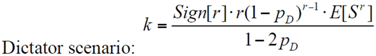
Rearranging (4’) gives:

(5’)

Equation (5) derives k from optimal giving, p_D , in the Dictator scenario. Equation (5’) derives k from the optimal threshold, p_U, in the Ultimatum game. Standard theories of fairness [10,11] assume that an individual has constant parameters for inequality aversion k, and risk aversion r, regardless of the game. We thus Equations (5) and (5’) to derive Equation (6), which shows giving in the Dictator game p_D, as an implicit function of the threshold in the Ultimatum game, p_U.

(6)

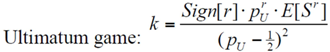
We can then derive prediction intervals for giving choices in the Dictator game from the observed threshold choice in the Ultimatum game, and vice versa. As shown in Equation (6), the relationship depends on the degree of risk aversion, r. We cannot determine the precise value of the risk aversion parameter r using our version of Holt & Laury [5], but we can predict the upper and lower bounds. Our predictions thus consist of intervals. We can thus determine if an observed choice in the Dictator (Ultimatum) game falls in the prediction interval derived from choices in the Ultimatum (Dictator) game. Figure 1 below illustrates our predictions.

Figure 1 shows the relationship between giving in the Dictator game on the x-axis and thresholds in the Ultimatum game on the y-axis. The graph shows the predicted choices in the Ultimatum (Dictator) game, given the choices in the Dictator (Ultimatum) game. The prediction depends on the risk preferences; hence, several lines are drawn in the graph. For example, given some choice in the Dictator game, on the x-axis, the corresponding thresholds in the Ultimatum game can be read on the y-axis. We can see that highly and very risk-averse people have a low, mostly flat curve, predicting low Ultimatum (near 0) thresholds for people who give strictly positive amounts over the typical range in the Dictator game. Risk-loving people have a slowly increasing curve that starts at a relative high point (0.22). Likewise, the graph can be used to predict Dictator giving, given their threshold choices in the Ultimatum game.13 Given the choice in the Ultimatum game, on the y-axis, the choice for giving in the Dictator game can be read on the x-axis.

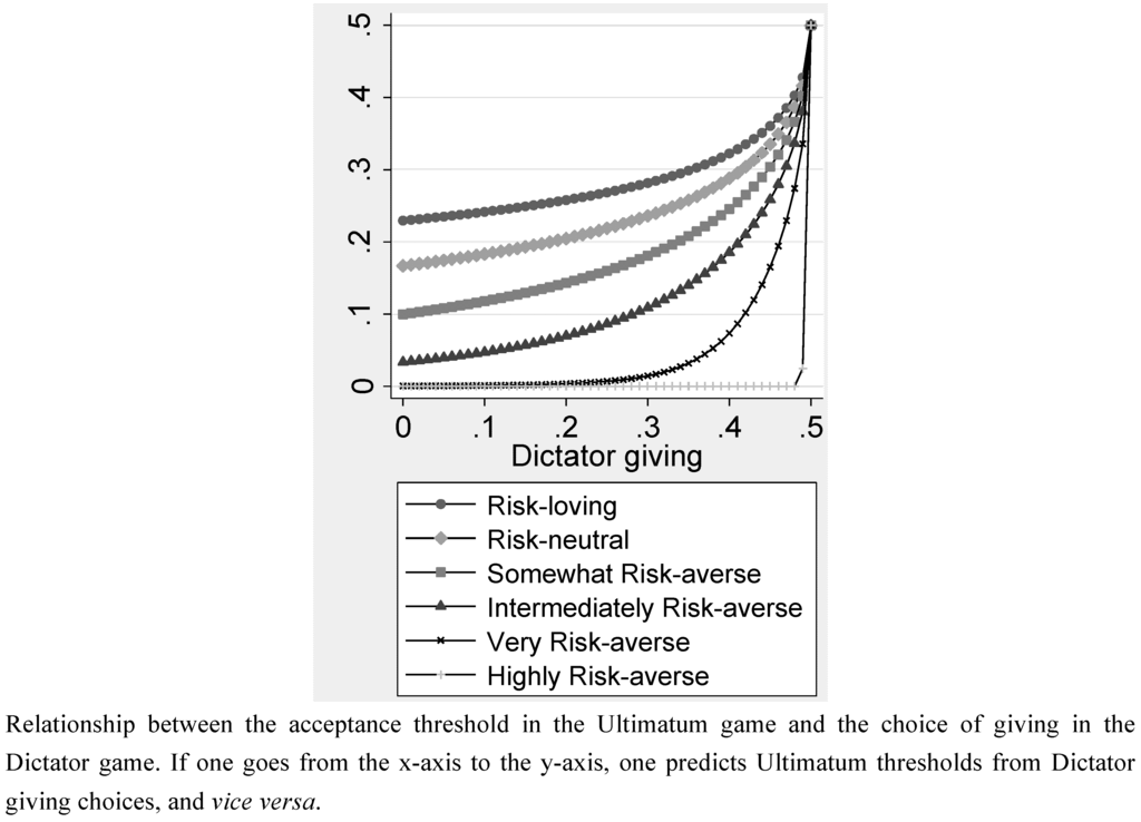
Figure 1. Predictions across games based on the ERC formula.

The relation between Ultimatum thresholds and Dictator giving is non-decreasing, as increases in inequality aversion will increase both Dictator giving and threshold in the Ultimatum game. We thus formulate:

Hypothesis 3: The choices in Dictator game (scenarios) and Ultimatum game (scenarios) are consistent.

3. Experimental Design and Implementation

To make hypotheses 1D and 1U experimentally testable, we specified endowments with increasing risk (“scenarios”) for Dictator and Ultimatum games. In particular, we provided endowments in the form of lottery tickets Sⁱ with Games 04 00208 i022

that realized a mean-preserving spread: Games 04 00208 i023

. In the low-risk condition, the lottery S^L takes the value of 900 or 1100, with ½ probability each. In the high-risk condition, the lottery S^H takes the value of 300 or 1700, with ½ probability each. In the no-risk condition, the lottery S^N is fixed at 1000. S^H is thus a mean-preserving spread of S^L, which is in turn a mean-preserving spread of S^N. Table 1 summarizes the different endowment risks.

Table 1. Operationalization of endowment risk.

**Table 1.** Operationalization of endowment risk.
	Possible realizations of the pie sizes Sⁱ (Dictator and Ultimatum)
Games	No-risk condition S^N	Low-risk condition S^L	High-risk condition S^H
Dictator	-	900 or 1100	300 or 1700
Ultimatum	1000	900 or 1100	300 or 1700

We employed two different subject pools: students of the Czech Technical University (CTU) and employees of Prague City Hall (CH). The subject pool consisted of 44 CH employees and 116 CTU students. 14 Since the two subject pools are different and individual characteristics such as risk attitudes play an important role in our theoretical analysis, we controlled for these variables.

The experiment was conducted at CERGE-EI on a portable experimental laboratory. We conducted 14 experimental sessions. Table 2 provides an overview of the experimental sessions:

Table 2. Overview of experimental sessions.¹⁵

**Table 2.** Overview of experimental sessions.¹⁵
Session	1	2	3	4	5	6	7	8	9	10	11	12	13	14	Total
Type of subjects	CTU	CTU	CTU	CTU	CTU	CTU	CTU	CTU	CTU^R	CTU^R	CH	CH	CH	CH
Number of subjects	14	12	16	14	12	16	16	16	16	16	10	8	16	10	192

The experiment was programmed in z-Tree [26]. The experimental instructions were in Czech. The experimenter first read descriptions of the four games (see Appendix A.5 and A.8 for the scripted instructions and the instructions in the z-Tree program). All subjects then had to correctly answer two questions on payoff calculations (see Appendix A.7) before they could proceed to the 17 choices that constituted the experiment. All games, and their scenarios, were framed in abstract terms. Five choices were about risk aversion (see Holt & Laury [5]; explained in more detail below). The computer program randomly selected ex post one of these five choices to be paid out. The twelve remaining choices were paid in full. The fully paid choices were the offer and acceptance threshold in the Ultimatum game (under no-risk, low-risk and high-risk realizations of the pie size), dictator giving in the Dictator game, and investment and return decisions in the Trust game (under low-risk and high-risk realizations of the pie size).16 Appendix A.6 contains the order in which these treatments were sequenced. No scenario realization was followed by the same scenario realization. We were aware that this kind of sequencing could lead to learning effects. Learning effects, however, are diminished when subjects are not informed about the outcomes of their decisions until the end of the session (e.g., Weber [27]), which is what occurred in our experiment. We thus ignore learning effects.

Each round random re-matching was used. As mentioned, subjects were informed of the outcomes of their decisions in the Dictator and Ultimatum games at the end of a session.17 The exchange rate was 1 CZK per 20 experimental currency units (ECU); payoff per subject ranged from 190 CZK to 620 CZK (payoffs were rounded up to the nearest multiple of ten), and the average payoff was slightly below 400 CZK.18 City Hall employees were paid an additional participation bonus of 150 or 200 CZK, as they had to commute to and from CERGE-EI and because sessions with CH employees lasted longer than those with student subjects (recall that the experiment proper started only once all participants in the session answered the questionnaire correctly, which on average took longer in the CH sessions).19 At the end of each session, we asked all subjects to identify their age and gender, and to report their disposable income.

Since the model predicts that risk aversion influences individual decision making, we categorized—as mentioned—all subjects according to their risk aversion through an additional scenario (see Scenario Four in the Instructions, in Appendix A.5). Similar to the procedure in Holt & Laury [5], subjects had to choose between a series of safer and riskier options. In the first choice, the safer option had a higher expected value (EV) than the corresponding riskier one. In the following choice, the riskier option had a higher expected value than the corresponding safer one. With every choice, the EV of the riskier choice grew faster than the EV of the corresponding safer one (see Table 3 below).20 Standard theory predicts that an agent will make at most one switch, if any, across the five choices. Since we wanted the decisions to be independent, we did not provide the choices in a back-to-back manner, but interspersed them as questions 2, 6, 10, 12, and 16 respectively with the other Scenario questions. Table 4 shows the risk aversion interval implied by the number of safe options the subject chooses.

Table 3. Elicitation of risk aversion.

**Table 3.** Elicitation of risk aversion.
		Safer option					EV		Riskier option					EV
Choice 1:	1000	if n>	40	,	1250	otherwise	1100	60	if n>	40	,	2400	Otherwise	996
Choice 2:	1000	if n>	50	,	1250	otherwise	1125	60	if n>	50	,	2400	Otherwise	1230
Choice 3:	1000	if n>	60	,	1250	otherwise	1150	60	if n>	60	,	2400	Otherwise	1464
Choice 4:	1000	if n>	70	,	1250	otherwise	1175	60	if n>	70	,	2400	Otherwise	1698
Choice 5:	1000	if n>	80	,	1250	otherwise	1200	60	if n>	80	,	2400	Otherwise	1932

n is a random number between 1 and 100 and determines the payoff of the chosen option for each of the choices

Table 4. Implied ranges of risk aversion r.

**Table 4.** Implied ranges of risk aversion r.
Number of safe choices	Range of Relative Risk Aversion r for		Risk Preference Classification
0	1.15	∞	Risk-loving
1	0.86	1.15	Risk-neutral
2	0.60	0.86	Somewhat Risk-averse
3	0.33	0.60	Intermediately Risk-averse
4	0.04	0.33	Very Risk-averse
5	–∞	0.04	Highly Risk-averse

4. Results

As in Holt & Laury [5], we use the number of safe choices to characterize and measure risk aversion in our sample. Only slightly more than half our subjects (52.7% of the CTU and CTU^R groups, and 54.5% of the CH group, i.e., 78 student subjects and 24 City Hall employees) made consistent choices.21 The risk preferences of subjects that made inconsistent choices is either undetermined, or within a very wide range. Since we compare subjects with low and high risk aversion in the range of Games 04 00208 i025

, we need to determine risk preferences precisely to test our hypotheses. We thus excluded inconsistent subjects from our sample in the regressions. Table A1 in Appendix A.1 shows the implied interval for risk aversion for all patterns of choice.

To test whether inconsistent subjects are different from consistent subjects, we ran two-sample Kolmogorov-Smirnov tests on socio-demographic variables. The distribution of inconsistent subjects does not differ for the sex and income variables, but differ for the variables Age, Time_to_answer (the control questions), and Safe (the number of safe choices) at a statistically (but not necessarily otherwise) significant level. On average, inconsistent subjects were 1 day older, took 55 seconds longer to answer the control questions, and made 0.9 fewer safe choices than consistent subjects. With the possible exception of the number of safe choices, these differences seem inconsequential.

We note that, on average, Dictator giving is 19%, Ultimatum offers are 43%, and Ultimatum thresholds are 26%, which is in line with previous findings in the literature (see Camerer [8] and Güth & Ortmann [9]).

Before analyzing our game data, we characterize the determinants of risk aversion for “consistent” subjects through regression analyses. Table 5 shows that socio-demographic characteristics influence risk aversion.

Table 5. Linear regression of risk aversion (defined as the safe choices) on socio-demographic variables.

**Table 5.** Linear regression of risk aversion (defined as the safe choices) on socio-demographic variables.
Variables	Effects
Income	–0.11 (0.06)**
Age	0.05 (0.03)
Female	*0.67 (0.37)**
Time_to_answer	0.06 (0.04)
City_Hall_employee	–0.63 (0.82)
CTU^R	0.07 (0.50)
Constant	2.23 * (0.75)**

Both students and City Hall employees are, on average, soundly risk-averse.22 City Hall employees are in general less risk-averse than students, but the difference is not significant (p > 0.42).23 Among our subjects, a person is predicted to be significantly more risk-averse when s/he earns a lower income (p = 0.043) or is female (p = 0.065), which is consistent with the literature (see Harrison & Rutström [31]). The variable Time_to_answer (the comprehension questions), which could be interpreted as a measure of cognitive ability, is not significant.

We use linear regression models clustered at the individual level to analyze the game data. We also use the robust Huber/White/sandwich estimator for the variance (Froot [32]).

4.1. Risk Attitude and Inequality Aversion (Hypothesis 1: Those with Higher Risk Aversion Show Higher Inequality Aversion in Their Responses.)

Table 6 contains the results of the linear regressions with clustered standard errors models. It contains the determinants of the amounts given in the Dictator game and the threshold level in the Ultimatum game. We test hypotheses 1D and 1U by regressing the percentage of the amount given in the Dictator game and the threshold level in the Ultimatum game on various variables of interest, as shown in Table 6. To measure the effect of risk aversion, we include a dummy variable, Somewhat_versus_highly_risk_averse, which equals zero for risk-loving and somewhat risk-averse subjects (0, 1 or 2 safe choices), and equals one for intermediately and highly risk-averse subjects (3, 4 and 5 safe choices).24

Table 6. Linear regression of giving on risk aversion and risk in the Dictator and Ultimatum games (with clustered errors).

**Table 6.** Linear regression of giving on risk aversion and risk in the Dictator and Ultimatum games (with clustered errors).
	Dictator				Ultimatum
	Model 1D1	Model 1D2	Model 1D3	Model 1D4	Model 1U1	Model 1U2	Model 1U3	Model 1U4
Dummy: Somewhat_versus_highly_risk_averse	9.59***	6.01*	10.49***	6.91*	5.81	4.68	6.73	5.59
Dummy: Somewhat_versus_highly_risk_averse	(3.60)	(3.46)	(3.92)	(3.92)	(3.96)	(4.08)	(4.10)	(4.24)
High_endowment_risk	−0.97	−0.97	0.30	0.30	3.71***	3.71***	5.40*	5.40*
	(1.81)	(1.83)	(3.58)	(3.62)	(1.24)	(1.25)	(2.93)	(2.95)
Low_endowment_risk					1.39	1.39	1.63	1.63
					(0.86)	(0.86)	(1.41)	(1.42)
Interaction Dummy: Somewhat_versus_highly_risk_averse x High_endowment_risk			−1.80	−1.80			−2.40	−2.40
			(4.15)	(4.19)			(3.19)	(3.21)
Interaction Dummy: Somewhat_versus_highly_risk_averse x High_endowment_risk							−0.34	−0.34
							(1.77)	(1.78)
Income		−0.00		−0.00		−0.64		−0.64
		(0.49)		(0.50)		(0.51)		(0.51)
Age		−0.32		−0.32		−0.21		−0.21
		(0.32)		(0.32)		(0.27)		(0.27)
Female		3.81		3.81		−1.95		−1.95
		(3.65)		(3.66)		(3.52)		(3.53)
Time_to_answer		1.80***		1.80***		0.61*		0.61*
		(0.37)		(0.38)		(0.32)		(0.32)
City_Hall_employees	8.73*	3.98	8.73*	3.98	−2.93	2.67	−2.93	2.67
	(4.62)	(6.36)	(4.63)	(6.38)	(4.08)	(7.08)	(4.09)	(7.10)
CTU^R	−3.87	−6.46	−3.87	−6.46	−4.38	−5.26	−4.38	−5.26
	(5.16)	(4.57)	(5.18)	(4.58)	(4.94)	(4.95)	(4.96)	(4.97)
Constant	10.55***	12.70*	9.91***	12.06*	20.18***	25.67***	19.53***	25.03***
	(3.27)	(7.45)	(3.51)	(7.20)	(3.71)	(7.28)	(3.80)	(7.28)
N	204	204			306	306
(Independent clusters)	(102)	(102)	204	204	(102)	(102)	306	306
R-squared	0.08	0.21	0.08	0.21	0.04	0.07	0.04	0.08

Robust standard errors in parentheses *** p < 0.01, ** p < 0.05, * p < 0.1.

The models 1D1 and 1U1 test the hypotheses 1D and 1U with the simplest specifications. In addition, we run regressions including the socio-demographic variables (models 1D2 and 1U2), and we also run—as robustness tests—regressions with interaction dummies to test if there is a significant interaction between endowment risk and risk aversion (models 1D3, 1D4, 1U3 and 1U4).

Model 1D1 provides support for hypothesis 1D: subjects with relatively high risk aversion give significantly (p < 0.01) more in the Dictator game.25 Model 1D2 shows that the effect is robust to the inclusion of the socio-demographic variables: the effect stays statistically significant (p < 0.09), albeit at a lower level of significance. Models 1D3 and 1D4 show that the interaction dummies, which have coefficients that are not significantly different from zero, do not affect the results.

Model 1U1 does not provide support for hypothesis 1U: while subjects with relatively high risk aversion set, in line with hypothesis 1U, higher thresholds in the Ultimatum game compared to those with relatively low risk aversion, the effect is not statistically significant. Surprisingly, endowment risk has a highly significant effect (p < 0.01) on the threshold level set in the Ultimatum game: an increase in endowment risk increases the threshold level. Model 1U3 shows that this effect occurs mostly independent of risk preferences: the effect of endowment risk on threshold remains significant (p = 0.07), albeit at a lower level of significance, in the presence of the interaction dummies that capture the interaction effects between endowment risk and risk aversion.

At first glance, there appears to be a subject-pool effect in Model 1D1, as City Hall employees tend to give significantly (p = 0.06) more in the Dictator game. Model 1D2 shows, however, that the subject-pool effect becomes insignificant when social-economic variables are included in the regression. In Model 1D2, the socio-economic variable Time_to_answer (the comprehension questions), which is possibly an indication of cognitive ability, is positive and significant (p < 0.01). We note that the coefficient of determination is quite low for all regressions in Table 6.

Even though, as mentioned, we cannot derive theoretical predictions for giving in the Ultimatum game, we ran a regression of Ultimatum giving on the same variables as in Table 6 and we found that Ultimatum giving does not depend on risk aversion.

4.2. Consistency within Games (Hypothesis 2: Increasing Endowment Risk does not have a Significant Effect)

Since we can only test hypotheses 2D and 2U by including somewhat risk-averse (but not risk-loving) subjects and very risk-averse (but not highly risk-averse) subjects, the number of observations is relatively small. In particular, we had to exclude not only inconsistent subjects, whose risk preference cannot be measured with sufficient precision to test hypothesis 1 and 2, but also highly risk-averse (5 safe choices) and risk-loving (0 safe choices) subjects, as they are not within the domain of hypothesis 2.26

To measure the effect of endowment risk, we include a dummy variable High_endowment_risk for testing hypothesis 2D and dummy variables High_endowment_risk and Low_endowment_risk for testing hypothesis 2U. Note also that the baseline is “low risk” in the Dictator game and “no risk” in the Ultimatum game.

Model 2D1 and 2U1 test the hypotheses with the simplest specifications. We also run regressions including the socio-demographic variables (models 2D2 and 2U2), and for hypothesis 2D we also run—as robustness tests—Tobit regressions (models 2D3 and 2D4) since many subjects made a choice of zero in the Dictator game.

Supporting hypothesis 2D, model 2D1 shows that the dummy for high-endowment risk is not statistically significant. The dummy for high-endowment risk is also insignificant in Model 2D2 (including the socio-demographic variables) and in models 2D3 and 2D4 (the robustness tests using Tobit regressions). Hypothesis 2D is thus supported by our data.

Contradicting hypothesis 2U, model 2U1 shows that both dummies for high-endowment risk (p < 0.01) and low-endowment risk (p = 0.07) are statistically significant.27 This suggests that participants with typical risk-aversion preferences set significantly higher thresholds under risk than under certainty. Model 2U2 shows that including socio-demographic variables does not change the results. Hypothesis 2U is thus not supported by our data.

Table 7. Linear regression of giving on risk aversion and endowment risk in the Dictator and Ultimatum games (with clustered errors).

**Table 7.** Linear regression of giving on risk aversion and endowment risk in the Dictator and Ultimatum games (with clustered errors).
	Dictator				Ultimatum
	Model 2D1	Model 2D2	Model 2D3(Tobit)	Model 2D4(Tobit)	Model2U1	Model2U2
High_endowment_risk	−0.83	−0.83	−0.92	−0.93	4.78***	4.78***
	(1.96)	(2.02)	(2.52)	(2.50)	(1.65)	(1.68)
Low_endowment_risk					3.18*	3.18*
					(1.73)	(1.76)
Income		1.16		2.09		−2.05
		(1.17)		(1.42)		(1.55)
Age		−0.49		−0.86		−0.08
		(0.43)		(0.59)		(0.54)
Female		5.32		9.48		−1.20
		(5.88)		(7.71)		(6.69)
Time_to_answer		2.06**		2.95**		0.55
		(0.89)		(1.25)		(1.36)
City_Hall_employees	14.90*	2.19	18.80*	−3.74	−4.21	16.33
	(7.99)	(12.07)	(9.62)	(15.63)	(8.58)	(17.12)
CTU^R	−3.53	−10.71	−8.78	−20.01	−1.88	−1.23
	(7.14)	(7.88)	(12.71)	(13.97)	(6.80)	(7.80)
Constant	15.59***	15.67	10.04*	12.45	24.47***	30.28*
	(3.22)	(10.53)	(5.18)	(13.50)	(3.86)	(15.00)
N	80	80	80	80	120	120
(Independent clusters)	(40)	(40)	(40)	(40)	60	60
R-squared (pseudo R-squared)	0.11	0.22	(0.02)	(0.04)	0.02	0.09

Robust standard errors in parentheses *** p < 0.01, ** p < 0.05, * p < 0.1

As in the regressions for testing hypothesis 1, there appears to be a subject-pool effect in Model 2D1 and 2D3, as City Hall employees tend to set significantly higher thresholds (p = 0.07) in the Ultimatum game. As in testing hypothesis 1, when social-economic variables are included in the regression (see Models 2D2 and 2D4), the subject-pool effect becomes insignificant and the variable Time_to_answer (the comprehension questions) becomes positive and significant (p = 0.03). We note that the coefficient of determination is quite low for all regressions in Table 7.

4.3. Consistency across Games (Hypothesis 3: Subjects Are Consistent between Games)

We used Equation (6) and subjects’ threshold choices in the Ultimatum game to derive prediction intervals from the observed threshold choices in the Ultimatum game for their giving choices in the Dictator game, and vice versa. This is a test of consistency between the two games on the individual level. Table 8 shows that subjects do not make consistent choices in the two games: the percentages of successful prediction are very low. Only 10% of the responses observed are within the predicted interval.28 We conclude that subjects are not consistent across games when measured on the individual level.

Table 8. Observed and predicted data on the individual level.

**Table 8.** Observed and predicted data on the individual level.
	Successful	Unsuccessful	Total
Predict D from U and visa versa	8 (10%)	75 (90%)	83 (100%)

Figure 2. Observed and predicted data on the aggregate level.

We also examined how well the ERC formulation predicts aggregate behavior. Figure 2 compares the predicted and observed choices for Dictator giving and Ultimatum thresholds, aggregated over all consistent subjects for both levels of endowment risk (low and high). Using the two-sample Kolmogorov-Smirnov tests, we reject the hypothesis that the observed and predicted distributions are the same for the Dictator game and the Ultimatum game (p < 0.001). The predicted distributions are thus poor approximations for the aggregate observed choices. Predictions at the aggregate level by and far fail. On the whole, this implies that subjects’ behavior is not consistent across games, on both the individual level or on the aggregate level. These findings are only partially in line with Blanco et al. [20], who found that behavior measured at the individual level was not consistent, but behavior measured at the aggregate level was fairly consistent. Our predictions were, however, more fine-grained than those in Blanco et al. [20]. They were thus subjected to a stricter, more demanding test for consistency. We also note that our findings are based on specification of the extended ERC formula. It is therefore possible that other specifications fare better (or worse). Our specification is, however, one of the simplest ways to implement constant risk-averse preferences. Better specifications would have more complicated forms.

5. Concluding Discussion

Summarizing the results, Hypothesis 1D and 2D are supported. Specifically, those who are more risk-averse are also more inequality-averse in the Dictator game (1D). Though the sign is correct for the Ultimatum game responder (IU), it is not significant, possibly because the number of observations was too low. This tentatively supports our first hypothesis, that those with higher risk aversion are more inequality-averse (and thus possess a stronger preference for fairness) than those with lower risk aversion. Our finding that more risk-averse people tend to be more inequality-averse is roughly in line with the results in Ferrer-i-Carbonell & Ramos [3] and Carlsson et al. [4] who used survey data and non-incentivized choices between imagined societies and lotteries. Our somewhat weaker results may reflect the fact that findings of inequality aversion are likely to be susceptible to “price” sensitivity, i.e., it is not difficult to be inequality-averse when there are no monetary consequences to making decisions.

Using the predictions derived from ERC theory, as implemented by a simple constant-relative-risk-aversion utility function (2), we find that endowment risk has no effect on giving in the Dictator game, confirming hypothesis 2D. Endowment risk does have a significant positive effect on the acceptance threshold in the Ultimatum game, contradicting hypothesis 2U. The effect, an increase in endowment risk leading to an increase in threshold, is in line with the prediction, but the size of the effect is much larger than predicted. This indicates that risk, which is not an ingredient of ERC theory, may affect acceptance thresholds in Ultimatum games.

We can thus conclude that the data corroborate the predictions from specification of the extended ERC formula for the Dictator game (1D and 2D), but not for the Ultimatum game (1U and 2U). We find that subjects are not consistent across games at the individual level, which contradicts hypothesis 3 but is consistent with the results of Blanco et al. [20]. At the aggregate level, we found that responses were not consistent across games, which is not in line with the results of Blanco et al. [20].

It is important to recall that people make inconsistent choices as viewed from the perspective of the theory that we use. One might conjecture that the functional form we used to incorporate risk preferences in the ERC formula may not be appropriate for the Dictator or Ultimatum game. The fact that our test of the effect of endowment risk on subject behavior, Hypothesis 2, is confirmed for the Dictator game, but contradicted for the Ultimatum game, suggests that the functional form we used may be appropriate for the Dictator game, but not for the Ultimatum game. We note that our test predicting the responses in one game from those in the other game is rather demanding test. These predictions are conditional on the risk preferences, which have been derived from our variant of the Holt & Laury [5] instrument. Basically, consistent choices in Hypothesis 3 thus require that the choices in three decision situations are consistent. That said, we know from other studies (like the one by Blanco et al. [20]) that others also have found that subjects make inconsistent choices.

Our data thus give tentative support to the claim that there is a positive relationship between risk aversion and fairness considerations. Our data also suggests that ERC theory, as formulated, does not seem particularly well suited to account for the effects of risk in the environment and risk preferences across the Dictator and Ultimatum games. The ERC formulation seems to fare better for the Dictator game.

We tested our theoretical predictions experimentally on two different subject pools: students of Czech Technical University—a subject pool we have drawn on previously that produced behavior in line with the behavior of student subjects elsewhere [33]—and employees of Prague City Hall. We generally did not find significant differences between the two groups, except for the regression of Dictator giving which indicated that employees of Prague City Hall give more in the Dictator game. This effect, however, is insignificant once socio-economic variables are incorporated in the regression. We included sessions where students were presented with the decision problems in a different order to control for order effects. These students show somewhat different responses on some of the variables of interest, indicating that order effects may play a role in the results of this study. The indicator variable for sessions with these students is, however, not significant in any of our tests, suggesting that order effects play a minor role in the results.

To summarize, we find that: (1) Those who are more risk-averse are also more inequality-averse in the Dictator game in that they give more. We believe this finding is novel. We find a similar result for the Ultimatum game but that result is statistically not significant; (2) Using the within-subject feature of our design, and in line with our theoretical prediction, varying risk does not influence behavior in the Dictator game, but does so in the Ultimatum game; (3) Using the within-subject feature of our design, subjects tend to make inconsistent decisions across games; this is true on the level of individuals (confirming the findings in Blanco et al. [20]) as well as in the aggregate (contradicting the findings in Blanco et al. [20]); (4) There are no subject-pool differences once we control for the elicited risk attitude and demographic variables that we collect.

^1.A reasonable intuition for that finding could be this: encountering states of inequality in the world makes one aware of the danger that one self may end up in some such state. This is likely to be the more threatening for a person the more s/he is risk-averse. This threat might activate, or intensify, inequality aversion.
^2.Cherry et al. [7] have demonstrated persuasively that the experimental results reported in the literature are dependent on both the degree of asset legitimacy and social distance. When the pie was not provided by the experimenter but had to be earned by their student dictators first (“asset legitimacy”), and when the game was also played under double anonymity (maximal “social distance”; see Hoffman et al. [12]), giving was as predicted by the standard economic assumption of selfishness. Bekkers [13] provides similar evidence through a field experiment. Smith [14] argues that asset legitimacy is an important challenge that experimental economists need to address.
^3.Engelmann & Strobel [15] presented an experimental test of the Bolton & Ockenfels and Fehr & Schmidt models which suggests that people, following Rawls’s theory of justice (Rawls [1]), want to maximize the welfare of the person who is the worst off (a form of other-regarding behavior); these authors (see also Engelmann & Strobel [16] for a balanced review of the literature and Engelmann [17] for an important caveat regarding the appropriate modeling of welfare maximization) identify the importance of efficiency concerns (defined as the sum of all payoffs in the game) as an explanatory variable. In their theory section, Charness & Rabin [18] use a social welfare criterion, which is defined as a weighted combination of minimal payoff (again, a form of other-regarding behavior) and the sum of all payoffs in the game. Cox & Sadiraj [19] provide a non-linear generalization of that model.
^4.Recent experimental work conducted in parallel by Güth et al. [21], Cappelen et al. [22], and Krawczyk & Le Lec [23], introduce theories or experimental results of distributive choice under risk. Güth et al. [21], continuing the work of Brennan et al. [24] and, using a within-subject design and incentive-compatible elicitation of valuations of 16 different prospects, find that individuals are self-oriented towards the social allocation of risk and delay and other-regarding with respect to expected payoffs. Cappelen et al. [22] use a two-stage dictator game to study to what extent, and under what circumstances, ex-ante fairness under risk is robust to ex-post redistribution. Krawzcyk & Le Lec [23] use a within-subject design and probabilistic versions of the dictator game that are manipulated along two dimensions (the relative cost of giving and the nature of the lottery) to try to tease out the relative merits of outcome-based and intention-based models of fairness under risk. All the models mentioned above were constructed under the assumption of pie sizes that are known ex ante.
^5.In addition, we also studied the so-called Trust game in such an environment (see Appendices A.5, A.6, and A.8). Assuming self-regarding preferences, the situation for responders in the Trust game is theoretically equivalent to that of dictators in a standard Dictator scenario. However, responders in our design and implementation of the Trust game cannot infer precisely the proposer’s initial decision (because the amount sent is multiplied by an unknown random factor X), and proposers cannot foresee the responders’ reaction. Proposers probably developed beliefs about responders’ behavior, but we were not able, given time constraints, to control for these during the experiment. We are therefore not able to theoretically derive the effects of risk preferences for proposing and responding in the Trust game and therefore decided not to include the Trust game in our analysis. We note that none of the relationships turned out significant for the Trust game.
^6.In principle, the recipient’s proposed share can also be determined in absolute terms. There are three reasons why we did not use absolute terms. First, in theories of fairness and reciprocity only relative terms matter. Second, an ex-ante allocation in absolute terms could result in a negative outcome for the decision maker (when the realized pie is small), which might trigger loss aversion and confound our results. Third, in the present paper we are not interested in optimal contract design (this could solve the preceding problem, but would also complicate our design beyond what seems feasible to implement.)
^7.Note that we have not used the ERC formulation to derive our hypotheses regarding the relation between risk aversion and inequality aversion in the Dictator and Ultimatum game, as this formulation is moot on the possible effects of risk aversion on inequality aversion. Predictions could be derived for people with different risk preferences, if the inequality aversion parameter k could be assumed to remain constant between different people with different risk preferences but with equal inequality aversion. This assumption does not hold as the inequality aversion parameter k conveys both an inequality aversion and an (unknown) rescaling effect. An increase in risk aversion is modeled by a transformation that results in a more concave utility function. This transformation also rescales the magnitude and the slope of the utility function and the parameter k needs to change to correct for this rescaling effect, making it impossible to deduce the individual inequality aversion effect. For example, using formula (4) below to estimate the parameter k shows that in our sample it ranges from an average of 0.2 (for highly risk-averse subjects) to 100 (for somewhat risk-averse subjects) to 5500 (for risk-loving subjects).
^8.This can easily be reformulated in terms of Fehr & Schmidt [11]; see Babicky [25].
^9.For standard stakes (such as the ones in our experiment) the constant-relative-risk-aversion form of the utility function can be rationalized experimentally by the results of Holt & Laury [5], p.1652, who suggest that it works as a “good approximation” of human behavior. This approximation simplifies our theoretical arguments considerably.
^10.Note that always . For any c, , any proportion of giving equal to is dominated by , as the latter proportion of giving results in higher utility, u[y], and equal inequality, .
^11.For risk-loving (r > 1) preferences, the relationship is inverted in the Ultimatum game, and depends on the values of k and r in the Dictator game. For highly risk-averse (r < 0) preferences, the relationship is inverted in the Dictator game and undefined in the Ultimatum game.
^12.See Appendix A.3.
^13.Note that for certain Ultimatum threshold levels no prediction of positive Dictator giving exists. For example, for Highly Risk-averse subjects, an Ultimatum threshold of 0.23 predicts zero Dictator giving. Ultimatum thresholds lower than 0.23 then predict negative Dictator giving, or “Dictator taking”. As Dictator taking was not a choice option in the experiment, the 14 observations where the Ultimatum threshold predicts Dictator taking were excluded from the analysis.
^14.We ran, at the tail end of the CTU sessions, two control sessions with an additional 32 CTU student subjects (sessions 9 and 10, indicated by CTU^R in Table 2). The subjects in the control group read the same instructions but were given a different ordering of decisions: all low-risk treatments were switched to high-risk treatments and vice versa. This control group, which did not take part in any of the other sessions, was conducted to control for order effects. Two-sample Kolmogorov-Smirnov tests suggest that the control group differs statistically significantly from the CTU group in at least two respects (age and the measure of cognitive ability that we will discuss below). It is not clear to us why we find these differences in age and cognitive ability, although it might be due to the fact that we ran those sessions at the tail end of the CTU sessions. In addition, using again two-sample Kolmogorov-Smirnov tests, we found the following significant differences in the decisions of the control group: they gave less in the Dictator game, made a lower offer in the Trust game, and sent less back in the Trust game. We include the data in our analysis below to determine the extent of the estimated treatment effects attributable to decision-order effects with a dummy variable, CTU^R. This dummy is not significant in any of the regressions in the results section.
^15.Each session contained an even number of participants, and was constrained by the maximum lab capacity of 16 people. We attempted to have at least 12 participants in each session but scheduling the four CH sessions turned out to be difficult. There is no a-priori reason that we can think of that would suggest this was more than a logistic inconvenience.
^16.Subjects were thus paid twice as recipients in the Dictator game (once for the low-risk and once for the high-risk condition).
^17.In the Trust game, subjects were informed of the amount they received once they were asked at the end of a session to make a decision as responder.
^18.When the experimental sessions were conducted, the exchange rate was about 23 CZK/1 USD, implying that our subjects—not counting appearance fees—earned on average 17–18 USD. The local purchasing power of these payoffs was about twice as much. Thus, it seems fair to say that the stakes were considerable for both students and City Hall employees. Since CH employees (and students) were told ex ante what average earning they could expect, we believe that only subjects that thought the money was worth their troubles signed up forthe experiment.
^19.Sessions lasted from 60 to 100 minutes, with student sessions typically being in the lower half and the CH sessions in the upper half of the interval.
^20.As in Holt & Laury [5], subjects were not told the expected value of the options they were given.
^21.We were aware ex ante (based, for example, on evidence reported in Hey & Orme [28]) that our procedure was likely to induce at least 25% inconsistent choices. Since we did not give our subjects the five risk-aversion measurement choices back to back, and did not give our subjects the EV of their options, with the benefit of hindsight, the fairly high percentage of inconsistent choices (not observed in the pilots in which we employed CERGE-EI students) is arguably not that surprising. It might simply reflect (as does also recent evidence on the stability of risk attitude assessment measures; see Dickhaut & Wilcox [29]) that other forms of elicitation may be confounded by subjects’ attempts to be consistent. Harrison et al. [30] interpret inconsistent choices as an indication that subjects are indifferent between the different gambles and that their risk preference is thus part of a “fatter” interval.
^22.The average number of safe choices is 3.5 for students and 3.2 for City Hall employees. This result is not out of line with other evidence (e.g., [5]), which suggests the vast majority of subjects are rather risk-averse. Given the considerable stakes in our experiment, our risk-attitude results seem sensible.
^23.We ran, as a robustness test, ordered logistic regressions with the number of safe choices as the independent variable: Signs are unaffected and the significance levels are roughly the same. The effect of being female, however, is no longer significant (p = 0.12). The difference between City Hall employees and students is not significant (p > 0.42).
^24.As robustness tests, we rerun the regressions using, to capture the difference in risk preferences, the variable safe, the number of safe choices a subject made, instead of the dummy Somewhat_versus_highly_risk_averse. With the variable safe, the significance is overall lower: the relationship for Dictator giving in Model 1 stays significant (p < 0.042), but not in Model 2 (p < 0.311).
^25.Running a Tobit regression, to account for the left-censoring of Dictator giving, gives the same significance levels for Models 1D1 and 1D3, and slightly higher ones for Models 1D2 and 1D4.
^26.Note that subjects with one safe choice include subjects who lean towards being somewhat risk-averse (0.86 < r < 1), subjects who are risk-neutral (r = 1), and subjects who lean towards being risk-loving (1 < r < 1.15); see Table 4. Since theory predicts that an increase in risk aversion has an effect for risk-loving subjects (decrease giving) that is opposite to that for risk-averse subjects (increase giving), the inclusion of these subjects should lead us to underestimate the increase in giving. However, effects on giving are very small round the point where risk-loving changes to risk aversion (r = 1), and we can thus expect that the resulting underestimation will be small. Indeed, running a regression excluding also the subjects with 1 safe choice does not change the results qualitatively.
^27.An F-test shows that the dummies for high and low endowment risk are not significantly different (p = 0.42).
^28.The success percentages are symmetric by design. The analysis in Table 8 excluded the 14 responses where the choice for the Ultimatum threshold predicted Dictator taking (giving a negative amount, which was not a possible choice in the experiment). Including these 14 responses, and accepting the closest possible Dictator giving choice, zero, as a correct prediction, increases the correct percentage of predictions somewhat, from the 10% reported in Table 8 to 20%.
^29.For each of the levels of risk aversion we studied, we created a grid of values for the inequality aversion parameter k and, using formula (4), calculated the optimal giving for each of the values of k, given the level of risk aversion and the level of risk. We use these coordinates to draw the figures in Figure A.2. We used a likewise procedure, using formula (4’) for drawing the figures in Figure A.3 for the Ultimatum games. We programmed the algorithms in Mathematica.

Acknowledgments

Funds for the experiment were provided by GAUK (V. Babicky) and GACR (A. Ortmann). S. van Koten is grateful for the Jean-Monnet Fellowship and the financial support of the Robert Schuman Center for Advanced Studies at the EUI in Florence. We are grateful to Prague City Hall for helping us contact municipal employees and we thank our colleague Petra Brhlikova for her help in the organization of the experimental sessions. We benefited from comments on early versions of this article by Martin Dufwenberg, Werner Güth, Glenn Harrison, David K. Levine, Ondřej Rydval, Jakub Steiner, and participants of GfeW, FUR, and ESA meetings. We are also grateful for the very constructive contributions of the two (anonymous) referees and the guest editor, Dorothea Herreiner, of GAMES. The usual caveat applies.

Conflict of Interest

The authors declare no conflict of interest.

References

Rawls, J. A Theory of Justice; Belknap Press of Harvard University Press: Cambridge, MA, USA, 1971. [Google Scholar]
Chambers, C.P. Inequality aversion and risk aversion. J. Econ. Theory 2012, 147, 1642–1651. [Google Scholar] [CrossRef]
Ferrer-i-Carbonell, A.; Ramos, X. Inequality aversion and risk attitudes. SOEP papers 271; DIW Berlin: Berlin, Germany, 2010. [Google Scholar]
Carlsson, F.; Daruvala, D.; Johansson-Stenman, O. Are people inequality-averse, or just risk-averse? Economica 2005, 72, 375–396. [Google Scholar] [CrossRef]
Holt, C.; Laury, S. Risk aversion and incentive effects. Am. Econ. Rev. 2002, 92, 1644–1655. [Google Scholar] [CrossRef]
Harrison, G.W.; Johnson, E.; McInnes, M.M.; Rutström, E.E. Risk aversion and incentive effects: Comment. Am. Econ. Rev. 2005, 95, 897–901. [Google Scholar] [CrossRef]
Cherry, T.; Frykblom, P.; Shogren, J. Hardnose the dictator. Am. Econ. Rev. 2002, 92, 1218–1221. [Google Scholar] [CrossRef]
Camerer, C.F. Behavioral Game Theory; Princeton University Press: Princeton, NJ, USA, 2003. [Google Scholar]
Güth, W.; Ortmann, A.A. Behavioral approach to distribution and bargaining. In Foundations and Extensions of Behavioral Economics: A Handbook; Altman, M., Ed.; Sharpe Publishers: New York, NY, USA, 2006; pp. 405–422. [Google Scholar]
Bolton, G.; Ockenfels, A. ERC: A theory of equity, reciprocity and competition. Am. Econ. Rev. 2000, 90, 166–193. [Google Scholar] [CrossRef]
Fehr, E.; Schmidt, K.A. Theory of fairness, competition and cooperation. Quart. J. Econ. 1999, 114, 817–868. [Google Scholar] [CrossRef]
Hoffman, E.; McCabe, K.; Smith, V.L. Social distance and other-regarding behavior in Dictator games. Am. Econ. Rev. 1996, 86, 653–660. [Google Scholar]
Bekkers, R. Measuring altruistic behavior in surveys: The all-or-nothing Dictator game. Surv. Res. Methods 2007, 1, 139–144. [Google Scholar]
Smith, V. Theory and experiment: What are the questions? J. Econ. Behav. Organ. 2010, 73, 3–15. [Google Scholar] [CrossRef]
Engelmann, D.; Strobel, M. Inequality aversion, efficiency and maximin preferences in simple distribution experiments. Am. Econ. Rev. 2004, 94, 857–869. [Google Scholar] [CrossRef]
Engelmann, D.; Strobel, M. Preference over income distributions—Experimental evidence. Public Finance Rev. 2007, 35, 285–310. [Google Scholar] [CrossRef]
Engelmann, D. How not to extend models of inequality aversion. J. Econ. Behav. Organ. 2012, 81, 599–605. [Google Scholar] [CrossRef]
Charness, G.; Rabin, M. Understanding social preferences with simple tests. Quart. J. Econ. 2002, 117, 817–869. [Google Scholar] [CrossRef]
Cox, J.; Sadiraj, V. Direct tests of individual preferences for efficiency and equity. Econ. Inquiry 2010, 50, 920–931. [Google Scholar]
Blanco, M.; Engelmann, D.; Normann, H.T. A within-subject analysis of other-regarding preferences. Games Econ. Behav. 2011, 72, 321–338. [Google Scholar] [CrossRef]
Güth, W.; Levati, M.V.; Ploner, M. On the social dimension of time and risk preferences. Econ. Inquiry 2008, 64, 261–272. [Google Scholar]
Cappelen, A.W.; Konow, J.; Sorensen, E.; Tungodden, B. Just luck: An experimental study of risk taking and fairness. Am. Econ. Rev. forthcoming.
Krawczyk, M.; Le Lec, F. “Give me a chance!” And experiment in social decision under risk. Exper. Econ. 2010, 13, 500–511. [Google Scholar] [CrossRef]
Brennan, G.; González, L.G.; Güth, W.; Levati, M.V. Attitudes toward private and collective risk in individual and strategic choice situations. J. Econ. Behav. Organ. 2008, 67, 253–262. [Google Scholar] [CrossRef]
Babicky, V. Fairness under risk: Insights from dictator games. CERGE-EI Working paper 2004, No. 217; The Center for Economic Research and Graduate Education, Economic Institute: Prague, Czech Republic, 2003. [Google Scholar]
Fischbacher, U. Z-Tree, Zurich toolbox for ready-made economic experiments. Exp. Econ. 2007, 10, 171–178. [Google Scholar] [CrossRef]
Weber, R.A. “Learning” with no feedback in a competitive guessing game. Games Econ. Behav. 2003, 44, 134–144. [Google Scholar] [CrossRef]
Hey, J.; Orme, C. Investigating Generalizations of expected utility theory using experimental data. Econometrica 1994, 62, 1291–1326. [Google Scholar] [CrossRef]
Dickhaut, J.; Wilcox, N. Elicitation of risk attitudes, a new assessment battery. 2010. Mimeo. [Google Scholar]
Harrison, G.W.; Lau, M.I.; Rutström, E.E.; Sullivan, M.B. Eliciting risk and time preferences using field experiments: Some methodological issues. In Field Experiments in Economics: Research in Experimental Economics; Harrison, G.W., Carpenter, J., List, J.A., Eds.; Emerald Group Publishing Limited: Bingley, UK, 2005; Volume 12, pp. 125–218. [Google Scholar]
Harrison, G.W.; Rutström, E.E. Risk aversion in the laboratory. In Research in Experimental Economics; Cox, J.C., Harrison, G.W., Eds.; Emerald: Bingley, UK, 2008; Volume 12, pp. 41–196. [Google Scholar]
Froot, K.A. Consistent covariance matrix estimation with cross-sectional dependence and heteroskedasticity in financial data. J. Finan. Quant. Anal. 1989, 24, 301–312. [Google Scholar] [CrossRef]
Rydval, O.; Ortmann, A. How financial incentives and cognitive abilities affect task performance in laboratory settings: An illustration. Econ. Lett. 2004, 85, 315–320. [Google Scholar] [CrossRef]

Appendix

A.1. Overview of Responses on the Holt-Laury Test

Table A1. The patterns of answers on the Holt-Laury test and the risk-aversion interval.

**Table A1.** The patterns of answers on the Holt-Laury test and the risk-aversion interval.
1^st	2^nd	3^rd	4^th	5^th	Interval	Risk aversion	Occurrence
Subjects that were consistent in their choices
RISKY	RISKY	RISKY	RISKY	RISKY	[1.15; +∞]	Risk-loving	9%
SAFE	RISKY	RISKY	RISKY	RISKY	[0.86; 1.15]	Risk-neutral	4%
SAFE	SAFE	RISKY	RISKY	RISKY	[0.60; 0.86]	Somewhat Risk-averse	4%
SAFE	SAFE	SAFE	RISKY	RISKY	[0.33; 0.60]	Intermediately Risk-averse	4%
SAFE	SAFE	SAFE	SAFE	RISKY	[0.04; 0.33]	Very Risk-averse	9%
SAFE	SAFE	SAFE	SAFE	SAFE	[−∞; 0.04]	Highly Riskaverse	24%
Subjects that had fat risk aversion intervals
SAFE	RISKY	RISKY	RISKY	SAFE	[−∞; 1.15]	Undeterminable	2%
SAFE	RISKY	RISKY	SAFE	RISKY	[0.04; 1.15]	Undeterminable	2%
SAFE	RISKY	RISKY	SAFE	SAFE	[−∞; 1.15]	Undeterminable	3%
SAFE	RISKY	SAFE	RISKY	RISKY	[0.33; 1.15]	Undeterminable	2%
SAFE	RISKY	SAFE	RISKY	SAFE	[−∞; 1.15]	Undeterminable	1%
SAFE	RISKY	SAFE	SAFE	RISKY	[0.04; 1.15]	Undeterminable	2%
SAFE	RISKY	SAFE	SAFE	SAFE	[−∞; 1.15]	Undeterminable	3%
SAFE	SAFE	RISKY	SAFE	RISKY	[0.04; 0.86]	Undeterminable	3%
SAFE	SAFE	RISKY	SAFE	SAFE	[−∞; 0.86]	Undeterminable	1%
SAFE	SAFE	SAFE	RISKY	SAFE	[−∞; 0.60]	Undeterminable	2%
RISKY	RISKY	RISKY	SAFE	RISKY	[0.04; +∞]	Undeterminable	4%
RISKY	RISKY	SAFE	RISKY	RISKY	[0.33; +∞]	Undeterminable	3%
RISKY	SAFE	RISKY	SAFE	RISKY	[0.04; +∞]	Undeterminable	4%
RISKY	SAFE	SAFE	RISKY	RISKY	[0.33 ; +∞]	Undeterminable	1%
Subjects that made contradictory choices
RISKY	RISKY	RISKY	RISKY	SAFE	[−∞; +∞]	Undeterminable	3%
RISKY	RISKY	RISKY	SAFE	SAFE	[−∞; +∞]	Undeterminable	4%
RISKY	RISKY	SAFE	SAFE	SAFE	[−∞; +∞]	Undeterminable	1%
RISKY	SAFE	RISKY	RISKY	SAFE	[−∞; +∞]	Undeterminable	1%
RISKY	SAFE	RISKY	SAFE	SAFE	[−∞; +∞]	Undeterminable	1%
RISKY	SAFE	SAFE	RISKY	SAFE	[−∞; +∞]	Undeterminable	1%
RISKY	SAFE	SAFE	SAFE	SAFE	[−∞; +∞]	Undeterminable	7%

A.2. Overview of the Socio-demographic Characteristics of the Subjects

Figure A.1 shows the distribution of our two subject pools conditional on the socio-demographic variables.

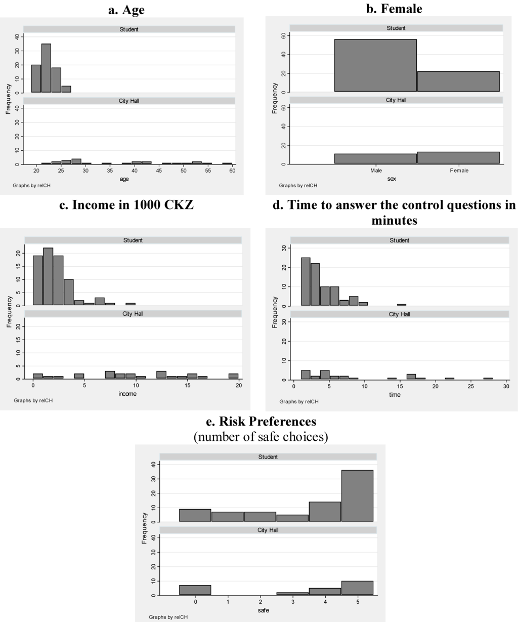
Figure A.1. Socio-demographic characteristics of City Hall employees and students.

As shown in the histograms, the socio-demographic characteristics differ markedly across the two subject pools, though there is also considerable overlap. In Figure A.1.e, we show the number of safe choices in the risk-attitude assessment task. The number of safe choices in tandem with Table 4 allows us to determine a subject’s degree of risk aversion.

A.3. Simulations on the Effect of Risk in the Dictator and Ultimatum Games on Decisions

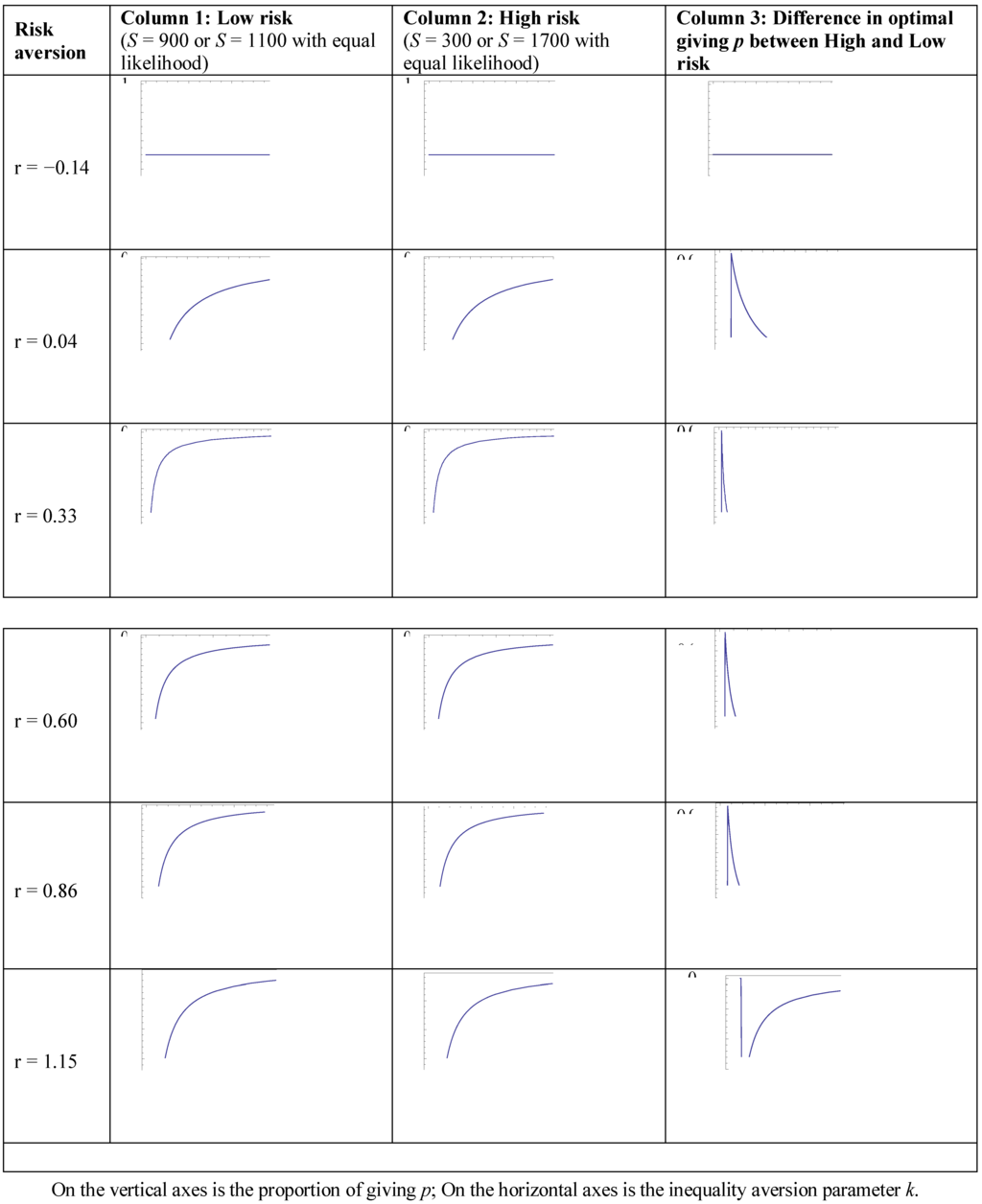
Figure A.2. Effect of risk on giving in the Dictator game.

Figure A.2 shows giving in the Dictator game as a function of the inequality aversion parameter k and the risk aversion parameter r for our formulation of the ERC model.29 The relationship is shown for the low-risk condition in the first column and for the high-risk condition in the second one. The third column shows the difference between the two graphs, which shows that the absolute difference is never larger than 0.03 for risk-averse subjects, and is never larger than 0.025 for risk-loving subjects. These differences are very small, and moreover, they are maxima over all possible inequality aversion parameters for the five degrees of risk aversion we consider. For example, differences are predicted to be no larger than 0.0043 for very risk-averse subjects (r = 0.04) and no larger than zero for highly risk-averse subjects (r = −0.14). We thus expect that risk will not affect dictator giving in the experiment.

Figure A.3 shows acceptance thresholds in the Ultimatum game as a function of the inequality aversion parameter k and the risk aversion parameter r for our formulation of the ERC model. The relationship is shown for the no-risk condition in the first column, for the low-risk condition in the second one, and for the high-risk condition in the third one. The fourth column shows the difference between the high-risk and the no-risk graphs (as they are the most different), and shows that for risk-loving subjects, the absolute difference is never larger than 0.004. The difference is never larger than 0.009 for somewhat risk-averse preferences. For very and highly risk-averse subjects, the difference can be substantial—up to almost 0.5. This is the result of a sudden switchover in the threshold from zero to close to 0.5 when the inequality aversion parameter k passes a certain value. With larger risk, the switchover occurs at a slightly higher k, thus resulting in a large difference. This difference is, however, predicted to exist only for a very narrow range of the inequality aversion parameter k. Over all values of k that are outside of this very narrow range, the difference is virtually zero. We thus expect that risk will not affect the acceptance thresholds set in the experiment.

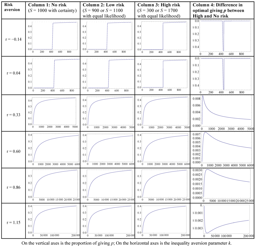
Figure A.3. Effect of risk on acceptance threshold in the Ultimatum game.

A.4. Prediction Errors on the Individual Level

Taking into account that subjects may have made errors in their choices, we look at the size of the error between the observed choices and the prediction interval.

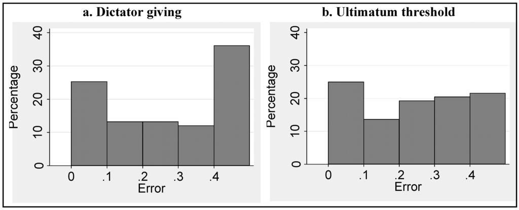
Figure A.4. Prediction error.

Figure A.4. shows that the overall prediction error is high both for Dictator giving and Ultimatum thresholds. The first bar in the histogram in Figure A.4.a accounts for all predictions of Dictator giving that have an error equal to 10 percentage points or less. It can be read from the vertical axis that these responses account for 25% of the total responses in the Dictator game. The first and second bar together account for all predictions that have an error equal to 20 percentage points or less: together they account for less than 40% of all responses in the Dictator game. Likewise, Figure A.4.b shows that the predictions for Ultimatum thresholds that have an error equal to 10 percentage points or less account for 25% of all responses and those that have an error equal to 20 percentage points or less account for 40% of all responses. The prediction error is thus considerable. We conclude that subjects are far from consistent across games when measured on the individual level.

A.5. Scripted Instructions

Welcome! You are about to participate in an economics experiment. You will be asked to make a series of decisions. Your decisions will have payoff consequences that will also depend on other participants’ decisions. You will be paid privately in cash immediately after the experiment is over. You will get 1 CZK for each 20 ECU (experimental currency units) that you earn during the experiment.

We ask that from now on you refrain from any communication, whether verbal or nonverbal, with other participants. If you have a question, raise your hand and an experimenter will come to assist you.

Throughout the experiment you will, for every single decision (where applicable), be matched randomly with one other participant. The probability that you will be matched with the same participant for more decisions is therefore rather low.

All in all you will be asked to make 17 decisions. You will be informed about the payoff consequences of any of these decisions only after your have made your last decision.

[Any questions?]

During the experiment we will use the following three basic scenarios (labeled One, Two, and Three). The computer is instructed to match you randomly with some other participant of the experiment in each of these three scenarios (for every decision you will get a new match). You will also be asked about your preferences (Scenario Four). In this Scenario your payoff cannot be affected by the decision of another participant.

Scenario One involves a pie of size S that is being divided between two participants that we call Participant A and Participant B. Task of Participant A is to split the pie of size S in any way he or she sees fit. Participant B is the recipient of what Participant A allocates; he or she will not make any decision in this scenario. Participant A will be asked to state her or his decision as a number between 0 and 100, i.e., as a percentage of pie size S that he or she allocates to Participant B.

[Any questions?]

Scenario Two involves a pie of size S that is being divided between two participants which we call Participant C and Participant D. Task of Participant C is to split the pie of size S in any way he or she sees fit. But now Participant D may either accept the offer or reject it. Participant C will be asked to state her or his decision of how to split the pie as a number between 0 and 100 (the “offer”), representing a percentage of pie size S that he or she offers to Participant D. Participant D will also be asked to state her or his decision whether he or she accepts the offer in a similar way as a number between 0 and 100 (the “acceptance threshold”) representing the minimal offer for which Participant D will not reject the offer. If the acceptance threshold of Participant D is higher than the offer that Participant C made, then the offer is not accepted, and both participants will be paid nothing for this scenario. Otherwise, they will be paid in accordance with the split that Participant C proposed.

[Any questions?]

Scenario Three involves Participants E and F. Participant E is endowed with 500 ECU out of which he or she can send any amount of his or her choice (from 0 to 500 ECU) to Participant F (the rest of the 500 ECU endowment stays on the account of Participant E). The amount sent to Participant F will be multiplied by a factor X before it reaches Participant F. It is then task of Participant F to split the amount received (i.e., X times the amount sent) in any way he or she sees fit. Participant E is the recipient of what Participant F allocates.

[Any questions?]

Scenario Four. The computer assigned to you at the beginning of the experiment a natural number N from 1 to 100 (any number 1, 2, 3, …, 100 is equally likely). This number will be revealed to you only at the end of the experiment. You will have to choose one of the two options “+” or “*”. On the screen, you have to fill a blank box with your choice of “+” or “*” and then press the “OK” button. Once you have pressed the “OK” button, you will not be able to go back. The computer is programmed to randomly select one of five such decisions you made during the whole experiment at the end of the experiment. For this purpose, the program uses a generator of random numbers. Choosing any of the five decisions in Scenario Four is equally likely. You will be paid at the end according to your choice in the selected decision and your personal N. (Note that in Scenario Four you do not interact with any other player.)

Example: choice +: 1000 ECU if N>40, 1250 ECU otherwise

or *: 60 ECU if N>40, 2400 ECU otherwise

(note that numbers will vary across decisions)

[Any questions?]

[Please turn your attention now to the computer screen but keep these hard copy instructions readily accessible.]

Thank you for participating in the experiment.

A.6. Sequencing of decisions

The sequencing of the decisions was the same for all participants, except those in sessions 9 and 10; see footnote 6 for an explanation:

Decision 1: Ultimatum proposal with no risk (pie size 1000)
Decision 2: Risk attitude measurement (n>40, i.e., Choice 1)
Decision 3: Dictator with low risk (pie size 900 or 1100)
Decision 4: Trust game sending with high risk (factor 1.2 or 2.8)
Decision 5: Ultimatum proposal with high risk (pie size 300 or 1700)
Decision 6: Risk attitude measurement (n>50, i.e., Choice 2)
Decision 7: Ultimatum threshold with high risk (pie size 300 or 1700)
Decision 8: Trust game sending with low risk (factor 1.8 or 2.2)
Decision 9: Ultimatum proposal with low risk (pie size 900 or 1100)
Decision 10: Risk attitude measurement (n>60, i.e., Choice 3)
Decision 11: Ultimatum threshold with low risk (pie size 900 or 1100)
Decision 12: Risk attitude measurement (n>70, i.e., Choice 4)
Decision 13: Dictator with high risk (pie size 300 or 1700)
Decision 14: Ultimatum threshold with no risk (pie size 1000)
Decision 15: Trust game return with high risk (factor 1.2 or 2.8)
Decision 16: Risk attitude measurement (n>80, i.e., Choice 5)
Decision 17: Trust game return with low risk (factor 1.8 or 2.2)

A.7. Control Questions

Consider scenario One with the total amount of S=200 ECU. You have the role of participant A and you made a choice of 84.

Question 1: What are your earnings from this scenario?
Question 2: What are the earnings of participant B, who has been selected randomly and assigned to you for this scenario. Please fill out your answer in the space above and confirm.

A.8. Instructions in the z-Tree Program

In the z-Tree program, participants were given instructions and referred to the printed instructions to guide their understanding of the decision tasks. In Table A.2 below, we give the full instructions as they appeared in the z-Tree program. In the left column are the original Czech instructions and in the right column the corresponding English translations. Each part starts with a code in brackets [], that identifies the task (Dictator, Ultimatum or Trust game or Holt-Laury task), the role for the participant (Proposer or Respondent role) and the degree of risk in the task (none, low, or high). The code in brackets was not presented to the participants.

Abbreviations used

D	Dictator Scenario
P	Proposer role
none	no-risk condition
U	Ultimatum Game
R	Respondent role
low	low-risk condition
T	Trust Game
high	high-risk condition
HL	Holt-Laury task

Table A.2. Instructions in the z-Tree program.

**Table A.2.** Instructions in the z-Tree program.
Original (Czech)	English translation
[Questionnaire] Nyni overime, ze vsichni porozumeli zakladnim scenarum, ktere popisuji instrukce. Odpovedi na nasledujici dve otazky nebudou mit dopad na Vasi vyplatu z experimentu, ale pokracovat budete moci jen po jejich spravnem zodpovezeni. Mate-li otazku, zvednete ruku a experimentator Vam prijde odpovedet. Uvazujte scenar Jedna s celkovou castkou S=200 ECU. (Pokud potrebujete, vratte se k tistenym instrukcim, ktere tento scenar popisuji.) Jste v roli ucastnika A a sve rozhodnuti jste vyjadril cislem 84. Otazka 1: Kolik je Vas zisk z pouziti tohoto scenare? Otazka 2: Kolik je zisk ucastnika B, ktery k Vam byl pro pouziti tohoto scenare nahodne prirazen? Vase odpovedi prosim vyplnte v jednotkach ECU do okenek vyse a potvrdte!	[Questionnaire] We will now ensure that everybody understood the basic scenarios from the instructions. Your answers on the two following questions will not have any effect on your earnings from the experiment, but you will be able to continue only after you have answered them correctly If you have an answer, please raise your hand and an experimenter will come. Consider scenario One with the total S=200 ECU (If you need to, you may return to the written instruction that describes this scenario) You have the role of participant A and you made a choice of 84. Question 1: What are your earnings from this scenario? Question 2: What are the earnings of participant B, who has been selected randomly and assigned to you for this scenario? Please fill out your answer in ECUs in the space above and confirm!
[U_P-none] Od nynejska budou mit vsechna Vase rozhodnuti dusledky na vysi Vasi vyplaty z tohoto experimentu. Proto davejte dobry pozor na ukoly, o ktere Vas budeme zadat. Uvazujte Scenar Dva s celkovou castkou S= 1000 ECU. (Pokud potrebujete, vratte se k tistenym instrukcim, ktere tento scenar popisuji.) Jste v roli ucastnika C a pro ucely scenare jste byl pocitacem nahodne prirazen k jinemu ucastnikovi experimentu. Rozhodnuti 1: Jaka je Vase nabidka? Prosim vyplnte Vasi odpoved do okenka a potvrdte!	[U_P-none] From now on, all your decisions will affect your earnings from this experiment. Therefore, pay close attention to the tasks we will present to you. Consider Scenario Two with the total S=200 ECU (If you need to, you may return to the written instruction that describes this scenario) You have the role of participant C and for this scenario you have been randomly assigned to another participant in this experiment. Decision 1: What is your proposal? Please fill out your answer in the space above and confirm!
[HL-40] Uvazujte scenar Ctyri. (Pokud potrebujete, vratte se k tistenym instrukcim, ktere tento scenar popisuji.) Volba "+": Ziskate 1000 ECU pokud N>40, jinak ziskate 1250 ECU Volba "*": Ziskate 60 ECU pokud N>40, jinak ziskate 2400 ECU Rozhodnuti 2: Kterou volbu preferujete?	[HL-40] Consider scenario Four (If you need to, you may return to the written instruction that describes this scenario) Choice “+”: You receive 1000 ECU when N>40, otherwise you receive 1250 ECU Choice “*”: You receive 60 ECU when N>40, otherwise you receive 2400 ECU Decision 2: What choice do you prefer?
[D] Nyni uvazujte scenar Jedna. (Pokud potrebujete, vratte se k tistenym instrukcim, ktere tento scenar popisuji.) Celkova castka S je nahodna a se stejnou pravdepodobnosti je bud S=900 ECU nebo S=1100 ECU. Jste v roli ucastnika A a pro ucely scenare jste byl pocitacem nahodne prirazen k jinemu ucastnikovi experimentu. Rozhodnuti 3: Jake je Vase rozhodnuti, kolik procent prevest?	[D] Now consider Scenario One. (If you need to, you may return to the written instruction that describes this scenario) The total amount S is random and is, with equal likelihood, equal to either S=900 ECU or S=1100 ECU. You have the role of participant A and for this scenario you have been randomly assigned to another participant in this experiment. Decision 3: What is your decision, how much as a percentage will you transfer?
[T_P] Uvazujte nyni scenar Tri. (Pokud potrebujete, vratte se k tistenym instrukcim, ktere tento scenar popisuji.) Faktor X je nahodne cislo a se stejnou pravdepodobnosti je bud X=1.2 nebo X=2.8. Jste v roli ucastnika E a pro ucely scenare jste byl pocitacem nahodne prirazen k jinemu ucastnikovi experimentu. Rozhodnuti 4: Kolik ECU posilate ucastnikovi F?	[T_P] Consider Scenario Three. (If you need to, you may return to the written instruction that describes this scenario) Factor X is a random number and is, with equal likelihood, equal to either X=1.2 or X=2.8. You have the role of participant E and for this scenario you have been randomly assigned to another participant in this experiment. Decision 4: How much ECU will you send to participant F?
[U_P-high] Uvazujte Scenar Dva. (Pokud potrebujete, vratte se k tistenym instrukcim, ktere tento scenar popisuji.) Celkova castka S je nahodna a se stejnou pravdepodobnosti je bud S=300 ECU nebo S=1700 ECU. Jste v roli ucastnika C a pro ucely scenare jste byl pocitacem nahodne prirazen k jinemu ucastnikovi experimentu. Rozhodnuti 5: Jaka je Vase nabidka? Prosim vyplnte Vasi odpoved do okenka a potvrdte!	[U_P-high] Consider Scenario Two. (If you need to, you may return to the written instruction that describes this scenario) The total amount S is random and is, with equal likelihood, equal to either S=300 ECU or S=1700 ECU. You have the role of participant C and for this scenario you have been randomly assigned to another participant in this experiment. Decision 5: What is your proposal?Please fill out your answer in the space above and confirm!
[HL-50] Uvazujte scenar Ctyri. (Pokud potrebujete, vratte se k tistenym instrukcim, ktere tento scenar popisuji.) Volba "+": Ziskate 1000 ECU pokud N>50, jinak ziskate 1250 ECU Volba "*": Ziskate 60 ECU pokud N>50, jinak ziskate 2400 ECU Rozhodnuti 6: Kterou volbu preferujete?	[HL-50] Consider scenario Four (If you need to, you may return to the written instruction that describes this scenario) Choice “+”: You receive 1000 ECU when N>50, otherwise you receive 1250 ECU Choice “*”: You receive 60 ECU when N>50, otherwise you receive 2400 ECU Decision 6: What choice do you prefer?
[U_R-high] Uvazujte Scenar Dva. (Pokud potrebujete, vratte se k tistenym instrukcim, ktere tento scenar popisuji.) Celkova castka S je nahodna a se stejnou pravdepodobnosti je budS=300 ECU nebo S=1700 ECU. Jste v roli ucastnika D a pro ucely scenare jste byl pocitacem nahodne prirazen k jinemu ucastnikovi experimentu. Rozhodnuti 7: Jaky je Vas prah akceptovatelnosti? Prosim vyplnte Vasi odpoved do okenka a potvrdte!	[U_R-high] Consider Scenario Two. (If you need to, you may return to the written instruction that describes this scenario) The total amount S is random and is, with equal likelihood, equal to either S=300 ECU or S=1700 ECU. You have the role of participant D and for this scenario you have been randomly assigned to another participant in this experiment. Decision 7: What is your proposal?Please fill out your answer in the space above and confirm!
[T_P-high] Uvazujte nyni scenar Tri. (Pokud potrebujete, vratte se k tistenym instrukcim, ktere tento scenar popisuji.) Faktor X je nahodne cislo a se stejnou pravdepodobnosti je bud X=1.8 nebo X=2.2. Jste v roli ucastnika E a pro ucely scenare jste byl pocitacem nahodne prirazen k jinemu ucastnikovi experimentu. Rozhodnuti 8: Kolik ECU posilate ucastnikovi F?	[T_P-high] Consider Scenario Three. (If you need to, you may return to the written instruction that describes this scenario) Factor X is a random number and is, with equal likelihood, equal to either X=1.8 or X=2.2. You have the role of participant E and for this scenario you have been randomly assigned to another participant in this experiment. Decision 8: How much ECU will you send to participant F?
[U_P-low] Uvazujte Scenar Dva. (Pokud potrebujete, vratte se k tistenym instrukcim, ktere tento scenar popisuji.) Celkova castka S je nahodna a se stejnou pravdepodobnosti je budS=900 ECU nebo S=1100 ECU. Jste v roli ucastnika C a pro ucely scenare jste byl pocitacem nahodne prirazen k jinemu ucastnikovi experimentu. Rozhodnuti 9: Jaka je Vase nabidka? Prosim vyplnte Vasi odpoved do okenka a potvrdte!	[U_P-low] Consider Scenario Two. (If you need to, you may return to the written instruction that describes this scenario) The total amount S is random and is, with equal likelihood, equal to either S=900 ECU or S=1100 ECU. You have the role of participant C and for this scenario you have been randomly assigned to another participant in this experiment. Decision 9: What is your proposal? Please fill out your answer in the space above and confirm!
[HL-60] Uvazujte scenar Ctyri. (Pokud potrebujete, vratte se k tistenym instrukcim, ktere tento scenar popisuji.) Volba "+": Ziskate 1000 ECU pokud N>60, jinak ziskate 1250 ECU Volba "*": Ziskate 60 ECU pokud N>60, jinak ziskate 2400 ECU Rozhodnuti 10: Kterou volbu preferujete?	[HL-60] Consider scenario Four (If you need to, you may return to the written instruction that describes this scenario) Choice “+”: You receive 1000 ECU when N>60, otherwise you receive 1250 ECU Choice “*”: You receive 60 ECU when N>60, otherwise you receive 2400 ECU Decision 10: What choice do you prefer?
[U_R-low] Uvazujte Scenar Dva. (Pokud potrebujete, vratte se k tistenym instrukcim, ktere tento scenar popisuji.) Celkova castka S je nahodna a se stejnou pravdepodobnosti je bud S=900 ECU nebo S=1100 ECU. Jste v roli ucastnika D a pro ucely scenare jste byl pocitacem nahodne prirazen k jinemu ucastnikovi experimentu. Rozhodnuti 11: Jaky je Vas prah akceptovatelnosti? Prosim vyplnte Vasi odpoved do okenka a potvrdte!	[U_R-low] Consider Scenario Two. (If you need to, you may return to the written instruction that describes this scenario) The total amount S is random and is, with equal likelihood, equal to either S=900 ECU or S=1100 ECU. You have the role of participant D and for this scenario you have been randomly assigned to another participant in this experiment. Decision 11: What is your acceptance threshold?Please fill out your answer in the space above and confirm!
[HL-70] Uvazujte scenar Ctyri. (Pokud potrebujete, vratte se k tistenym instrukcim, ktere tento scenar popisuji.) Volba "+": Ziskate 1000 ECU pokud N>70, jinak ziskate 1250 ECU Volba "*": Ziskate 60 ECU pokud N>70, jinak ziskate 2400 ECU Rozhodnuti 12: Kterou volbu preferujete?	[HL-70] Consider scenario Four (If you need to, you may return to the written instruction that describes this scenario) Choice “+”: You receive 1000 ECU when N>70, otherwise you receive 1250 ECU Choice “*”: You receive 60 ECU when N>70, otherwise you receive 2400 ECU Decision 12: What choice do you prefer?
[D-high] Nyni uvazujte scenar Jedna. (Pokud potrebujete, vratte se k tistenym instrukcim, ktere tento scenar popisuji.) Celkova castka S je nahodna a se stejnou pravdepodobnosti je bud S=300 ECU nebo S=1700 ECU. Jste v roli ucastnika A a pro ucely scenare jste byl pocitacem nahodne prirazen k jinemu ucastnikovi experimentu. Rozhodnuti 13: Jake je Vase rozhodnuti, kolik procent prevest?	[D-high] Now consider Scenario One. (If you need to, you may return to the written instruction that describes this scenario) The total amount S is random and is, with equal likelihood, equal to either S=300 ECU or S=1700 ECU. You have the role of participant A and for this scenario you have been randomly assigned to another participant in this experiment. Decision 13: What is your decision, how much as a percentage will you transfer?
[U_R-none] Uvazujte Scenar Dva s celkovou castkou S= 1000 ECU. (Pokud potrebujete, vratte se k tistenym instrukcim, ktere tento scenar popisuji.) Jste v roli ucastnika D a pro ucely scenare jste byl pocitacem nahodne prirazen k jinemu ucastnikovi experimentu. Rozhodnuti 14: Jaky je Vas prah akceptovatelnosti? Prosim vyplnte Vasi odpoved do okenka a potvrdte!	[U_R-none] Consider Scenario Two. With the amount S=1000 ECU. (If you need to, you may return to the written instruction that describes this scenario) You have the role of participant D and for this scenario you have been randomly assigned to another participant in this experiment. Decision 14: What is your acceptance threshold? Please fill out your answer in the space above and confirm!
[T_R-high] Uvazujte nyni scenar Tri. (Pokud potrebujete, vratte se k tistenym instrukcim, ktere tento scenar popisuji.) Faktor X je nahodne cislo a se stejnou pravdepodobnosti je bud X=1.2 nebo X=2.8. Jste v roli ucastnika F a pro ucely scenare jste byl pocitacem nahodne prirazen k jinemu ucastnikovi experimentu. Obdrzel jste castku ECU (to je X krat mnozstvi poslane ucastnikem E, ktery k Vam byl pro toto rozhodnuti nahodne prirazen.) Rozhodnuti 15: Kolik ECU prevadite zpet na ucastnika E?	[T_R-high] Consider Scenario Three. (If you need to, you may return to the written instruction that describes this scenario) Factor X is a random number and is, with equal likelihood, equal to either X=1.2 or X=2.8. You have the role of participant F and for this scenario you have been randomly assigned to another participant in this experiment. You received the amount ECU: … (this is X times the amount send by the participant E, who was for this decision randomly assigned to you.) Decision 15: How much ECU will you send back to participant E?
[HL-80] Uvazujte scenar Ctyri. (Pokud potrebujete, vratte se k tistenym instrukcim, ktere tento scenar popisuji.) Volba "+": Ziskate 1000 ECU pokud N>80, jinak ziskate 1250 ECU Volba "*": Ziskate 60 ECU pokud N>80, jinak ziskate 2400 ECU Rozhodnuti 16: Kterou volbu preferujete?	[HL-80] Consider scenario Four (If you need to, you may return to the written instruction that describes this scenario) Choice “+”: You receive 1000 ECU when N>80, otherwise you receive 1250 ECU Choice “*”: You receive 60 ECU when N>80, otherwise you receive 2400 ECU Decision 16: What choice do you prefer?
[T_R-low] Uvazujte nyni scenar Tri. (Pokud potrebujete, vratte se k tistenym instrukcim, ktere tento scenar popisuji.) Faktor X je nahodne cislo a se stejnou pravdepodobnosti je bud X=1.8 nebo X=2.2. Jste v roli ucastnika F a pro ucely scenare jste byl pocitacem nahodne prirazen k jinemu ucastnikovi experimentu. Obdrzel jste castku ECU(to je X krat mnozstvi poslane ucastnikem E, ktery k Vam byl pro toto rozhodnuti nahodne prirazen.) Rozhodnuti 17: Kolik ECU prevadite zpet na ucastnika E?	[T_R-low] Consider Scenario Three. (If you need to, you may return to the written instruction that describes this scenario) Factor X is a random number and is, with equal likelihood, equal to either X=1.8 or X=2.2. You have the role of participant F and for this scenario you have been randomly assigned to another participant in this experiment. You received the amount ECU: … (this is X times the amount send by the participant E, who was for this decision randomly assigned to you.) Decision 17: How much ECU will you send back to participant E?
[Demographics] Zatimco my a pocitacovy program urcujeme celkove vydelky z dnesniho experimentu, prosime Vas odpovedet na nekolik otazek o Vas. Vsechna data budou povazovana za prisne duverna a budou pouzita pouze pro tuto studii. Po vyplneni a az Vas experimentator pozada, predstupujte jednotlive s Vasim obcanskym prukazem (pripadne jinou ID kartou) k vyplate. -Vase rodne cislo -Kolik je Vas mesicni disponibilni prijem (to je, kolik penez muzete utratit pote, co zaplatite za sve ubytovani)?	[Demographics] While we an the computer program are calculating the total earnings from todays experiment, we would like to ask you to answer some questions. All data will be considered as strictly confidential a will be used only for this study. After you have filled out the questionnaire and once the experimenter ask you to, please come one by one to the pay desk with your identity card (or with another form of ID). -Your birth number -How much is your monthly disposable income (that is, how much can you spend after you have paid for lodging?)
[Results] Vase N bylo Z rozhodnuti 2,6,10,12,16 bylo nahodne vybrano rozhodnuti Z toho rozhodnuti Vas vydelek cinil ECU Z rozhodnuti 1 jste vydelal ECU Z rozhodnuti 3 jste vydelal ECU V roli ucastnika B jste z rozhodnuti 3 Vam nahodne prirazeneho ucastnika A vydelal ECU Z rozhodnuti 4 jste vydelal ECU Z rozhodnuti 5 jste vydelal ECU Z rozhodnuti 7 jste vydelal ECU Z rozhodnuti 8 jste vydelal ECU Z rozhodnuti 9 jste vydelal ECU Z rozhodnuti 11 jste vydelal ECU Z rozhodnuti 13 jste vydelal ECU V roli ucastnika B jste z rozhodnuti 13 Vam nahodne prirazeneho ucastnika A vydelal ECU Z rozhodnuti 14 jste vydelal ECU Z rozhodnuti 15 jste vydelal ECU Z rozhodnuti 17 jste vydelal ECU	[Results] Your N was From decisions 2, 6, 10, 12, 16 has been randomly chosen decision: … From this decision you earning is in ECU: … From decision 1 you earned in ECU: … From decision 3 you earned in ECU: … In the role of participant B, you have for decision 3 received from a randomly assigned participant A in ECU: … From decision 4 you earned in ECU: … From decision 5 you earned in ECU: … From decision 7 you earned in ECU: … From decision 8 you earned in ECU: … From decision 9 you earned in ECU: … From decision 11 you earned in ECU: … From decision 13 you earned in ECU: … In the role of participant B, you have for decision 3 received from a randomly assigned participant A in ECU: … From decision 14 you earned in ECU: … From decision 15 you earned in ECU: … From decision 17 you earned in ECU: …

© 2013 by the authors; licensee MDPI, Basel, Switzerland. This article is an open access article distributed under the terms and conditions of the Creative Commons Attribution license (http://creativecommons.org/licenses/by/3.0/).

Share and Cite

MDPI and ACS Style

Van Koten, S.; Ortmann, A.; Babicky, V. Fairness in Risky Environments: Theory and Evidence. Games 2013, 4, 208-242. https://doi.org/10.3390/g4020208

AMA Style

Van Koten S, Ortmann A, Babicky V. Fairness in Risky Environments: Theory and Evidence. Games. 2013; 4(2):208-242. https://doi.org/10.3390/g4020208

Chicago/Turabian Style

Van Koten, Silvester, Andreas Ortmann, and Vitezslav Babicky. 2013. "Fairness in Risky Environments: Theory and Evidence" Games 4, no. 2: 208-242. https://doi.org/10.3390/g4020208

APA Style

Van Koten, S., Ortmann, A., & Babicky, V. (2013). Fairness in Risky Environments: Theory and Evidence. Games, 4(2), 208-242. https://doi.org/10.3390/g4020208

Article Menu

Fairness in Risky Environments: Theory and Evidence

Abstract

1. Introduction

2. Theoretical Predictions for Fairness in Risky Environments

2.1. Risk Attitude and Inequality Aversion

2.2. Consistency within Games

2.3. Consistency across Games

3. Experimental Design and Implementation

4. Results

4.1. Risk Attitude and Inequality Aversion (Hypothesis 1: Those with Higher Risk Aversion Show Higher Inequality Aversion in Their Responses.)

4.2. Consistency within Games (Hypothesis 2: Increasing Endowment Risk does not have a Significant Effect)

4.3. Consistency across Games (Hypothesis 3: Subjects Are Consistent between Games)

5. Concluding Discussion

Acknowledgments

Conflict of Interest

References

Appendix

A.1. Overview of Responses on the Holt-Laury Test

A.2. Overview of the Socio-demographic Characteristics of the Subjects

A.3. Simulations on the Effect of Risk in the Dictator and Ultimatum Games on Decisions

A.4. Prediction Errors on the Individual Level

A.5. Scripted Instructions

A.6. Sequencing of decisions

A.7. Control Questions

A.8. Instructions in the z-Tree Program

Abbreviations used

Share and Cite

Article Metrics

Article Access Statistics

Further Information

Guidelines

MDPI Initiatives

Follow MDPI