Two Pricing Mechanisms in Sponsored Search Advertising

Abstract

Sponsored search advertising has grown rapidly since the last decade and is now a significant revenue source for search engines. To ameliorate revenues, search engines often set fixed or variable reserve price to in influence advertisers’ bidding. This paper studies and compares two pricing mechanisms: the generalized second-price auction (GSP) where the winner at the last ad position pays the larger value between the highest losing bid and reserve price, and the GSP with a posted reserve price (APR) where the winner at the last position pays the reserve price. We show that if advertisers’ per-click value has an increasing generalized failure rate, the search engine’s revenue rate is quasi-concave and hence there exists an optimal reserve price under both mechanisms. While the number of advertisers and the number of ad positions have no effect on the selection of reserve price in GSP, the optimal reserve price is affected by both factors in APR and it should be set higher than GSP.

1. Introduction

In sponsored search advertising each advertiser bids for keywords and purchases sponsored links relevant to his business from Google, Yahoo!, MSN, and their partners. When an internet user searches a specific term or keyword in a search engine, sponsored links may be displayed in the front page in addition to search result links. Whenever a sponsored link is clicked, its sponsor or advertiser will pay the search engine a fee, called cost per-click (CPC), for the service of leading consumers to his web site. Many corporations and small businesses take advantage of this affordable, targeted advertising method. Google reported an annual revenue of $37.91 billion in 2011, and 96% of it came from its advertising business (Google Investor Relations [1]).

Sponsored links associated with a particular keyword are sold through auction where each advertiser submits a bid to the search engine for his willingness to pay for a CPC. In 2002 Google introduced AdWords, which stipulates that an advertiser in position i pays a CPC that equals the bidding price of the advertiser in position $i+1$ plus a minimum increment. Named the generalized second-price (GSP) auction, this mechanism has become the building block in sponsored search advertising. The revenue created by each sponsored link to the search engine is determined by the advertiser’s CPC and the click through rate (CTR), i.e., average number of clicks the link receives per unit time. There are a limited number of sponsored links that a search engine can display on each page, and the links at the top of a page receive significantly more clicks than ones at the bottom (Brooks [2]). For instance, ad links on Google’s first page are most valuable, of which up to 3 links are on the top of search results and at most 8 links are on the right side.

To screen advertisers and improve the quality of sponsored links, search engines set up reserve price called minimum bid to each keyword auction. Advertisers must pay at least the minimum bid per click to maintain the active status of their ad links. Since early 2008 Yahoo! has no longer fixed its minimum bid at $0.10 and started imposing variable minimum bids for some keywords (Yahoo! Search Marketing Blog [3]). Later Google introduced the first page bid estimate to approximate the minimum CPC needed to show a sponsored link in the first page, which is “based on placement in the last position on the right hand side of Google. This may be anywhere between positions 1 and 11, depending on how many ads are shown for that query" (Google Adwords Help [4]). If a link appears in the bottom-most position among top links above search results, or if it is the only top link, the advertiser pays the amount of the CPC threshold (Google Adwords Help [5]). Both first page bid estimate and CPC threshold are announced to advertisers and updated regularly. To avoid various nomenclatures, we use reserve price to represent the CPC that is charged to the advertiser winning the last ad position.

Motivated by the economy in sponsored search advertising and intrigued by the opaqueness of its practice, we study and compare two pricing mechanisms for selling multiple heterogeneous ad positions. The first is the GSP auction defined by Edelman et al. [6] and Varian [7] where the bidder winning the lowest position pays the larger value between reserve price and the highest losing bid. The second, which we suspect being adopted in practice, especially for selling top sponsored links above search results, is basically a hybrid between an auction and a posted price mechanism. It is similar to GSP except for stipulating that the winner of lowest position pays the posted reserve price regardless the number of positions sold. Calling it the GSP auction with posted reserve price (APR), we attempt to address the following questions: (i) Does the optimal reserve price exist for each mechanism? Is it the same as the one that applies to single-item auctions? (ii) In addition to bidder’s private value, are there other factors that affect the selection of optimal reserve price? (iii) Which mechanism creates more expected revenue for the search engine?

Although GSP has been widely used in the literature to analyze sponsored search advertising, it is based on a static game that ignores the dynamic nature of the auction. The search engine determines a reserve price before the auction starts while no ad position has been sold. In the reality, however, the search engine may review periodically as to whether the current reserve price needs to be revised given part of or all ad positions have been occupied. In a separate paper (Yang et al. [8]), we will show that in the dynamic setting, the constant reserve price, suggested by GSP, is not optimal. On the other hand, the optimal reserve price derived from APR is able to capture the influence of the number of positions sold.

The rest of the paper is organized as follows. Section 2 reviews the related literature and highlights our contribution. Section 3 starts with the discussion on equilibrium strategy in GSP and APR. We then study these two pricing mechanisms for the search engine and derive the optimal reserve prices. Comparison and analysis are presented in Section 4. Concluding remarks are placed in Section 5.

2. Literature Review and Contribution of the Paper

Reserve price for auctions has been studied long before sponsored search advertising came into practice. Myerson [9], Riley and Samuelson [10] consider single-item auctions where risk neutral bidders have independent private values. They discover that the item should be awarded to the bidder who has the highest value if and only if it exceeds a critical threshold. Maskin and Riley [11] extend the analysis to auctions with multiple identical items and show that the seller should set a fixed reserve price independent from the number of bidders. Bulow and Roberts [12] use marginal revenue analysis to associate auction theory with economic fundamentals. They let $F(·)$ and $f(·)$ denote the probability distribution and density functions of bidders’ willingness to pay, respectively. If the monopolistic seller sets a take-it-or-leave-it price r, then the expected quantity of sales would be $q(r)=1-F(r)=\overline{F}(r)$. They show that the seller should disqualify those bidders with negative marginal revenues, and the value that renders zero marginal revenue is the optimal reserve price. Explicitly, it is the solution of

$$\begin{array}{c}\hfill MR(r)=\frac{d}{dq}[r·q(r)]=r-\frac{\overline{F}(r)}{f(r)}=0\end{array}$$

(1)

A complication of sponsored search advertising is the heterogeneity of auction items or ad positions. As the click-through rate is descending with positions, each advertiser chooses a position (or none) to maximize his payoff, and equilibrium becomes a natural issue. Since GSP auctions are infinitely repeated games, the sets of equilibria can be very large and analysis of possible equilibrium strategies becomes intractable. Edelman et al. [6] focus on a static GSP in which bids are stabilized. They find that the GSP auction generally does not have equilibrium in dominant strategies, and truth-telling does not lead to an equilibrium. They define a locally envy-free equilibrium of the simultaneous game induced by GSP where each advertiser cannot be better off by swapping bids with the advertiser ranked one position above. Varian [7] proposes a notion of symmetric Nash equilibrium (SNE) and shows that the bids at the lower bound of SNE are the same as the bids under the locally envy-free equilibrium. Varian [7] also shows that there is a compelling reason for players to bid at the lower bound of SNE. Empirical evidence indicates that actual bidding observed in Google’s ad auction is in the neighborhood of lower bound of SNE.

While research on sponsored search auction has been popular, study on its reserve price is sporadic. Edelman and Schwarz [13] show that (1) applies to the optimal reserve price for a generalized English auction. Defined in Edelman et al. [6] with more details, the generalized English auction starts with a clock showing the current price, increasing over time from a reserve price. Bidders participating in the auction are willing to pay at least the reserve price. As price goes up bidders start dropping out. One’s bid is the price shown on the clock when he quits. The auction ends until the last bidder remains, who wins the top ad position paying the price shown on the clock when the next-to-last one quits. The next-to-last bidder wins the second position and pays the bid price of the third-highest bidder, and so on. In light of this definition, in the generalized English auction, if the number of qualified bidder does not exceed the number of positions, the one winning the last position pays the reserve price per click; otherwise, he pays the larger value between the reserve price and the highest losing bid. In Theorem 1 we prove the same optimality condition (1) for a generalized English auction when the number of bidders is uncertain. However, in the APR mechanism when the winner of the lowest position pays the reserve price regardless of the number of slots sold, the optimal reserve price does not satisfy (1).

In this article we study two pricing mechanisms, GSP and APR, in selling multiple heterogeneous ad positions. In both mechanisms advertiser at position i pays the bid price of the advertiser at position $i+1$. The only difference is that in APR the one occupying the last slot pays the posted reserve price while in GSP he pays the larger value between reserve price and the highest losing bid. Since the number of bidders in each period may vary, we assume that the bidding stream follows a Poisson distribution. The number of qualified bidders, hence, is also a Poisson variable endogenously affected by the reserve price. Poisson arrival assumption is standard in revenue management literature (Xiao and Yang [14], Feng and Xiao [15]), and it is often adopted by economists. Wang [16] compares an auction with a posted-price mechanism selling a uniquely indivisible object when buyers arrive randomly according to a Poisson process. He finds that if the auctioning cost is absent, the auction always creates more revenue than posted-price selling. As the empirical study by Varian [7] at Google shows that advertisers tend to follow bidding strategies at the lower bound of symmetric Nash equilibrium, we focus on the lower bound of SNE (or equivalently locally envy-free strategies) and maximize the search engine’s long-term expected revenue rate with reserve price as a control variable. We prove that in either mechanism the expected revenue rate is quasi-concave if advertisers’ per-click value has an increasing generalized failure rate function. In GSP the optimal reserve price satisfies the condition of (1), while in APR, optimality condition suggests that the optimal reserve price should be set higher than the one defined in GSP. It depends on the number of positions, the number of advertisers, and their per-click values. From the dynamic point of view, this is reasonable because when the search engine periodically reviews its reserve price, the number of positions available for sale is unlikely constant. As a result, the reserve price should reflect it and be adjusted accordingly. The minimum bids stated by search engines (see Yahoo! Search Marketing Help [17]) corroborate our findings.

3. Pricing Mechanisms

The keywords auctions in Yahoo! and Google are repeated games in which bidders gradually learn the value of their competitors and adjust their bids accordingly. The set of equilibria in repeated games can be very large and the strategies leading to such equilibria are complex. As Edelman et al. [6] note, it may not be reasonable to expect advertisers capable of executing such strategies, especially when they manage thousands of keywords. Edelman and Schwarz [13] show that a static game with certain equilibrium strategy set is able to capture many important characteristics of the underlying dynamic game. Hence, we study a simultaneous-move one-shot auction assuming that (1) bidders are likely to learn all relevant information about each other’s value over time; (2) bidders submit their stable bids in equilibrium. A drawback of this simplification is it implies that the auction always begins with the same number of positions available prior to arrivals of bidders. In reality, the auction is continuous and the number of positions remaining for sale varies from time to time.

In practice, Google ranks advertisers based on the product of each advertiser’s bid and his “quality score”. The quality score is determined by a number of factors including the CTR, the keyword’s relevancy to the advertiser’s business and the quality of his web site. Varian [7] and Edelman et al. [6] both show that incorporating quality score in the study does not provide much additional insight. Hence, in our paper both GSP and APR determine winners solely based on bid prices.

3.1. Equilibrium in GSP and APR

An exogenously given k ad positions are for sale through auction. There are n advertisers endogenously affected by the reserve price r. The expected CTR received by ad position i is ${\alpha }_i$. Since top positions receive higher CTR than lower positions, we have ${\alpha }_i>{\alpha }_{i+1}$ for $1\le i\le k-1$ and ${\alpha }_i=0$ for $i>k$. Advertisers are risk-neutral possessing independent private information. They may have distinct willingness to pay for one click, but for each advertiser, his per-click value stays the same even if his ad appears in different positions. Let $b^{(i)}$, $v_{(i)}$ and $I(i)$ denote the bid price, per-click value and identity of the ith highest bid, respectively. If $b^{(i)}$ is greater than the reserve price, both mechanisms allocate the ith position to the advertiser with the ith highest bid, $I(i)$, where $i\in \{1,...,min(n,k)\}$. When the ith link is clicked by a user, advertiser $I(i)$ pays the search engine an amount that equals the next highest bid, $b^{(i+1)}$. If advertiser $I(i)$ happens to be the winning bidder in the lowest ranking, he pays the posted reserve price in APR or the larger value between reserve price and the highest losing bid in GSP. The revenue received by the search engine from the ith sponsored link is ${\alpha }_i{b}^{(i+1)}$ and the surplus to advertiser $I(i)$ is ${\alpha }_i(v_{(i)}-b^{(i+1)})$.

Definition 1 (Varian [7]) In a symmetric Nash equilibrium (SNE) bid prices satisfy

$$\begin{array}{c}\hfill {\alpha }_i(v_{(i)}-b^{(i+1)})\ge {\alpha }_j(v_{(i)}-b^{(j+1)}),\forall iandj\end{array}$$

(2)

Varian shows that if a set of prices is an SNE, then it is a Nash equilibrium (NE). He further shows that if the state of advertiser $I(i)$ satisfies condition (2) for position $j=i+1$ and $j=i-1$, then it satisfies (2) for all j. Hence, one only needs to compare each advertiser’s current position with its two adjacent slots.

Since the advertiser in position i does not want to move down, we have

$$\begin{array}{ccc}\hfill {\alpha }_i(v_{(i)}-b^{(i+1)})& \ge & {\alpha }_{i+1}(v_{(i)}-b^{(i+2)})\hfill \end{array}$$

(3)

On the other hand, the advertiser in position $i+1$ has no incentive to move one slot up. Thus,

$$\begin{array}{ccc}\hfill {\alpha }_{i+1}(v_{(i+1)}-b^{(i+2)})& \ge & {\alpha }_i(v_{(i+1)}-b^{(i+1)})\hfill \end{array}$$

(4)

The above two inequalities lead to

$$\begin{array}{c}\hfill \frac{({\alpha }_i-{\alpha }_{i+1})v_{(i+1)}+{\alpha }_{i+1}{b}^{(i+2)}}{{\alpha }_i}\le b^{(i+1)}\le \frac{({\alpha }_i-{\alpha }_{i+1})v_{(i)}+{\alpha }_{i+1}{b}^{(i+2)}}{{\alpha }_i}\end{array}$$

(5)

Note that any $b^{(i+1)}$ satisfying the above inequalities is an equilibrium bid. Hence, there is a range of such equilibrium strategies. From the practical point of view, this seems to make the equilibrium bids indeterminate. Varian [7] examines the boundary cases by choosing the upper and lower bounds in (5), which yields

$$\begin{array}{ccc}\hfill b^{(i+1)}& =& \frac{({\alpha }_i-{\alpha }_{i+1})v_{(i+1)}+{\alpha }_{i+1}{b}^{(i+2)}}{{\alpha }_i},\text{(lower bound)}\hfill \end{array}$$

(6)

$$\begin{array}{ccc}\hfill b^{(i+1)}& =& \frac{({\alpha }_i-{\alpha }_{i+1})v_{(i)}+{\alpha }_{i+1}{b}^{(i+2)}}{{\alpha }_i},\text{(upper bound)}\hfill \end{array}$$

(7)

It is easy to see that the bidding strategy at the lower bound belongs to the locally envy-free equilibrium (Edelman et al. [6]) and it is in fact the lowest-revenue envy-free equilibrium (Edelman and Schwarz [13]). Equations based on such an equilibrium with various names can be found in several literatures including the self-selection condition in the priority pricing mechanism studied in Harris and Raviv [18], and the indifference constraint in Wilson [19] that considers the myopic incentive constrained pricing.

Questions that follow naturally are why advertisers are destined to the lower bound of SNE and how their bids converge to this particular point? Varian [7] explains that it is more reasonable for the bidder to compare his current payoff with what he will end up if he outbids the advertiser one slot above him. He argues that among all SNE strategies, the lower bound strategy is the most appealing one to advertisers since it defines the lowest bid prices that render each agent the most advantageous position. Varian also shows that the lower bound strategy is closely related to the two-sided matching problem discussed in Roth and Sotomayor [20]. Edelman et al. [6] show that if the dynamic game ever converges to a static vector of bids, that static equilibrium should correspond to a locally envy-free equilibrium of the static game induced by the GSP. In addition, both Edelman et al. [6] and Varian [7] show that in the dominant-strategy Vickrey–Clarke–Groves equilibrium, the position and CPC of each advertiser coincide with those in the lower bound of the SNE, and the outcome is the best for advertisers but worst for the search engine. Hence, the lower bound strategy provides incentives to advertisers and it is most likely attainable. Edelman and Schwarz [13] further show that the lower bound strategy in a GSP with complete information, capturing behaviors in an incomplete information game, can be viewed as a valid approximation. The empirical analysis conducted by Varian [7] over a random sample of 2425 auctions at Google also shows that there is demonstrable evidence indicating that the actual bidding in Google’s ad auction converges to the neighborhood of the equilibrium strategy at the lower bound of SNE.

In the rest of the paper we use the term of (lowest-revenue) envy-free equilibrium and lower bound of the SNE interchangeably. Any equilibrium strategy examined will satisfy the lower bound constraint (6).

3.2. Optimal Reserve Price in Sponsored Search Advertising

We consider n qualified advertisers whose per-click values are represented by an n-dimensional random vector ($X_1,X_2,\cdots ,X_n$). The realization of these n values is ($x_1,x_2,\cdots ,x_n$). Rearranging $x_1,x_2,\cdots ,x_n$ in an increasing order so that $x_{(1)}\le x_{(2)}\le \cdots \le x_{(n)},$ where $x_{(1)}=min\{x_1,x_2,\cdots ,x_n\}$, $x_{(2)}$ is the second smallest value in the n-tuple, and so on. The function $X_{(i)}$ of ($X_1,X_2,\cdots ,X_n$) that takes on the $x_{(i)}$ in each possible sequence ($x_1,x_2,\cdots ,x_n$) of values assumed by ($X_1,X_2,\cdots ,X_n$) is known as the ith order statistic.

Let $X_1,X_2\cdots ,X_n$ be identical and independent random variables with common probability density function $f(x)$ and distribution function $F(x)$. We approximate the total number of advertisers by a Poisson random variable with a mean λ. When the reserve price is equal to r, the probability for each potential advertiser to participate in the auction is $\overline{F}(r)=1-F(r)$ and $\lambda \overline{F}(r)$ is the average number of qualified bidders. One can regard $\lambda \overline{F}(r)$ as the demand function for ad positions and λ as the maximum arrival rate when the reserve price is set to zero. Hence, the probability of having n eligible bidders per unit time is equal to $\frac{{[\lambda \overline{F}(r)]}^n}{n!}{e}^{-\lambda \overline{F}(r)}$. Following Lariviere and Porteus [21], we define $h(x)=\frac{f(x)}{\overline{F}(x)}$ as the failure rate of $F(·)$ and $g(x)=xh(x)$ as the generalized failure rate. As

$$g(x)=x\frac{f(x)}{\overline{F}(x)}=-\frac{x}{dx}\frac{d\overline{F}(x)}{\overline{F}(x)}$$

the generalized failure rate $g(x)$ is the absolute value of the price elasticity.

For a qualified bidder j its per-click value satisfies the following conditional distribution function

$$F_r(x)=P[X_j\le x|X_j\ge r]=\frac{P[r\le X_j\le x]}{P[X_j\ge r]}=\frac{F(x)-F(r)}{\overline{F}(r)}$$

Hence, the marginal probability density function of $X_{(i)}$ is given by

$$f_{(i)}(x)=\frac{n!}{(i-1)!(n-i)!}{[F_r(x)]}^{i-1}{[1-F_r(x)]}^{n-i}\frac{f(x)}{\overline{F}(r)}$$

(8)

and the expectation of $X_{(i)}$ can be written as

$$E[X_{(i)}]={\int }_r^{\infty }x{f}_{(i)}(x)dx=\frac{n!}{(i-1)!(n-i)!}{\int }_r^{\infty }x{[F_r(x)]}^{i-1}{[1-F_r(x)]}^{n-i}\frac{f(x)}{\overline{F}(r)}dx$$

(9)

Let p be the CPC the advertiser at the last position pays, i.e., $b^{(n\wedge k)+1}=p$, where $n\wedge k=min(n,k)$. Note that in GSP p is the larger value between r and the highest losing bid while $p=r$ in APR. Equation (6) enables us to derive $b^{(i)}$ recursively. For $i<n\wedge k$,

$$b^{(i)}=\frac{{\alpha }_i{b}^{(i+1)}+({\alpha }_{i-1}-{\alpha }_i)X_{(n-i+1)}}{{\alpha }_{i-1}}$$

(10)

When there are k positions offered and n advertisers qualified, search engine’s revenue per unit time is given by

$$R(n,n\wedge k)=p{\alpha }_{n\wedge k}+\sum _{l=1}^{n\wedge k-1}{\alpha }_l{b}^{(l+1)}$$

(11)

In view of (10), for $l<n\wedge k-1$, we have

$$\begin{array}{ccc}\hfill {\alpha }_l{b}^{(l+1)}& =& {\alpha }_{l+1}{b}^{(l+2)}+({\alpha }_l-{\alpha }_{l+1})X_{(n-l)}\hfill \\ & =& p{\alpha }_{n\wedge k}+({\alpha }_l-{\alpha }_{l+1})X_{(n-l)}+\cdots +({\alpha }_{n\wedge k-1}-{\alpha }_{n\wedge k})X_{(n-n\wedge k+1)}\hfill \end{array}$$

which can be substituted into (11) to form a linear function of order statistics:

$$R(n,n\wedge k)=p(n\wedge k){\alpha }_{n\wedge k}+\sum _{l=1}^{n\wedge k-1}l({\alpha }_l-{\alpha }_{l+1})X_{(n-l)}$$

(12)

As the true per-click values of advertisers are unknown to the search engine, $R(n,n\wedge k)$ is uncertain and its expectation can be depicted as

$$E[R(n,n\wedge k)]=p(n\wedge k){\alpha }_{n\wedge k}+\sum _{l=1}^{n\wedge k-1}l({\alpha }_l-{\alpha }_{l+1})E[X_{(n-l)}]$$

Conditioning on the number of qualified bidders n, the expected revenue rate is

$$\Psi (r)=\sum _{n=0}^{\infty }E[R(n,n\wedge k)]\frac{{[\lambda \overline{F}(r)]}^n}{n!}{e}^{-\lambda \overline{F}(r)}$$

(13)

The objective of the search engine is to maximize $\Psi (r)$ by choosing an optimal reserve price $r^{*}$.

3.2.1. GSP

Lemma 1 In the lower bound of the locally envy-free equilibrium, the expected revenue rate to the search engine from the static generalized second-price auction (GSP) for sponsored search advertising is

$$\begin{array}{ccc}\hfill {\Psi }_A(r)& =& r\sum _{n=1}^k({\alpha }_1+\cdots +{\alpha }_n)\frac{{[\lambda \overline{F}(r)]}^n}{n!}{e}^{-\lambda \overline{F}(r)}+\sum _{n=1}^k{\int }_r^{\infty }\left(\sum _{l=1}^n{\alpha }_l-n{\alpha }_n\right)\frac{{[\lambda \overline{F}(x)]}^n}{n!}{e}^{-\lambda \overline{F}(x)}dx\hfill \end{array}$$

$$\begin{array}{ccc}& +& r({\alpha }_1+\cdots +{\alpha }_k)\sum _{n=k+1}^{\infty }\frac{{[\lambda \overline{F}(r)]}^n}{n!}{e}^{-\lambda \overline{F}(r)}+\sum _{n=k+1}^{\infty }{\int }_r^{\infty }\sum _{l=1}^k{\alpha }_l\frac{{[\lambda \overline{F}(x)]}^n}{n!}{e}^{-\lambda \overline{F}(x)}dx\hfill \end{array}$$

(14)

The proof of Lemma 1 and all other proofs are placed in the appendix.

In a GSP, the revenue contributions from n bidders consist of two parts: the minimum amount to win a position, represented by

$$r({\alpha }_1+\cdots +{\alpha }_{n\wedge k})\frac{{[\lambda \overline{F}(r)]}^n}{n!}{e}^{-\lambda \overline{F}(r)}$$

and the extra to secure each winning position, represented by

$$[({\alpha }_1-{\alpha }_n)+\cdots +({\alpha }_{n-1}-{\alpha }_n)]{\int }_r^{\infty }\frac{{[\lambda \overline{F}(x)]}^n}{n!}{e}^{-\lambda \overline{F}(x)}dx$$

if $n\le k$ and

$$({\alpha }_1+\cdots +{\alpha }_k){\int }_r^{\infty }\frac{{[\lambda \overline{F}(x)]}^n}{n!}{e}^{-\lambda \overline{F}(x)}dx$$

if $n>k$.

The standard regularity condition in the auction literature requires an increasing failure rate (IFR) (Maskin and Riley [11]), while a milder condition is an increasing generalized failure rate (IGFR). The assumption that the distribution function has an IGFR is prevalent in pricing and revenue management literature (Ziya et al. [22] and Lariviere [23]). It ensures either a unimodal or quasi-concave revenue function when selling a single product. Our model extends the result to the scenario with heterogeneous products.

Theorem 1 If the value per click of each advertiser is a variable with IGFR, then (i) ${\Psi }_A(r)$ is a quasi-concave function; (ii) the optimal reserve price $r^{*}$ is given as the solution to the equation

$$\begin{array}{c}\hfill r^{*}-\frac{1-F(r^{*})}{f(r^{*})}=0\end{array}$$

(15)

Note that the generalized failure rate is the absolute value of price elasticity. IGFR implies that consumers respond to a price increase more negatively when the reserve price is high than when it is low. In sponsored search advertising, it means that the demand reduction in ad links resulted from a mark-up is increasing in the reserve price, which reflects the behavior of rational advertisers. Thus, the assumption of IGFR in Theorem 1 is minor and reasonable.

In auctions of selling a single item or multiple homogeneous items, the optimal reserve price solves Equation (1) (Bulow and Roberts [12]). Theorem 1 shows that it is also the optimality condition for the static GSP with heterogeneous items. Notice that condition (15) is equivalent to $g(r)=1$ and $g(r)$ is the absolute value of price elasticity of demand. As $g(r)$ is an increasing function of r, it makes perfect sense for (15): increase the reserve price when demand is inelastic until the elasticity reaches unity; further increases will reduce the revenue.

Although English auctions with multiple heterogeneous items and endogenous entries have been studied in the literature, to our knowledge, there has not been theoretical development for an analytical solution of the optimal reserve price. The significance of Theorem 1, hence, is twofold. It provides the optimal reserve price for a static generalized English auction where the payment schedule for the last winning bidder is dependent on the number of bidders; second, it shows that heterogeneity among objects alone does not necessarily lead to a varied optimal reserve price.

3.2.2. APR

Lemma 2 In the locally envy-free equilibrium, the expected revenue rate to the search engine from APR for sponsored search advertising is

$$\begin{array}{c}\hfill {\Psi }_P(r)=\sum _{n=1}^{\infty }\left[r\sum _{l=1}^{n\wedge k}{\alpha }_l\frac{{[\lambda \overline{F}(r)]}^n}{n!}{e}^{-\lambda \overline{F}(r)}+{\int }_r^{\infty }\left(\sum _{l=1}^{n\wedge k}{\alpha }_l-(n\wedge k){\alpha }_{n\wedge k}\right)\frac{{[\lambda \overline{F}(x)]}^n}{n!}{e}^{-\lambda \overline{F}(x)}dx\right]\end{array}$$

(16)

When there are n bidders in the auction, their contributions consist of two parts: the minimum amount they have to pay to win a position, represented by

$$r({\alpha }_1+\cdots +{\alpha }_{n\wedge k})\frac{{[\lambda \overline{F}(r)]}^n}{n!}{e}^{-\lambda \overline{F}(r)}$$

and the premium paid for securing each winning position, represented by

$$[({\alpha }_1-{\alpha }_{n\wedge k})+\cdots +({\alpha }_{n\wedge k-1}-{\alpha }_{n\wedge k})]{\int }_r^{\infty }\frac{{[\lambda \overline{F}(x)]}^n}{n!}{e}^{-\lambda \overline{F}(x)}dx$$

For example, the advertiser taking the first position in the auction must pay ${\alpha }_{1}r\frac{{[\lambda \overline{F}(r)]}^n}{n!}{e}^{-\lambda \overline{F}(r)}$ per unit time to pass the revenue threshold defined by the reserve price, and an extra amount $({\alpha }_1-{\alpha }_{n\wedge k}){\int }_r^{\infty }\frac{{[\lambda \overline{F}(x)]}^n}{n!}{e}^{-\lambda \overline{F}(x)}dx$ to be on top. In general, the heterogeneity among items for sale drives each consumer to select the most advantageous one for him. If all items are identical (with the same CTR or quality), no one will pay more than the reserve price.

The marginal revenue function can be verified as

$$\begin{array}{c}\hfill {\Psi }_P^{\prime }(r)=[1-\frac{rf(r)}{\overline{F}(r)}]\sum _{n=1}^{k}n{\alpha }_n\frac{{[\lambda \overline{F}(r)]}^n}{n!}{e}^{-\lambda \overline{F}(r)}+k{\alpha }_k\sum _{n=k+1}^{\infty }\frac{{[\lambda \overline{F}(r)]}^n}{n!}{e}^{-\lambda \overline{F}(r)}\end{array}$$

Theorem 2 If each advertiser’s per-click value is a random variable with IGFR, then ${\Psi }_P(r)$ is quasi-concave and there exists a unique reserve price that maximizes the expected revenue rate. The optimal reserve price $r^{*}$ is given as the solution to the equation

$$\begin{array}{c}\hfill r^{*}-[1+\theta (r^{*})]\frac{1-F(r^{*})}{f(r^{*})}=0\end{array}$$

(17)

where

$$\theta (r^{*})=\frac{k{\alpha }_k{\sum }_{n=k+1}^{\infty }\frac{{[\lambda \overline{F}(r^{*})]}^n}{n!}}{{\sum }_{n=1}^{k}n{\alpha }_n\frac{{[\lambda \overline{F}(r^{*})]}^n}{n!}}$$

The optimality condition (17) of reserve price in APR clearly differs from (15) in GSP, which can be written as $g(r)=1+\theta (r)$. The perturbation factor $\theta (r)$ shows that it is directly related to the bidder population λ, the number of available ad positions k, and the distribution of bidders’ valuation function F. The proof of Theorem 2 shows that $\theta (r)$ is decreasing in r. With the assumption of IGFR, there is an optimal reserve price that achieves the maximal expected revenue rate.

4. Discussions

4.1. Revenue Comparison

The only difference between GSP and APR discussed in the preceding section is what the kth highest bidder pays when there are at least k qualified advertisers. In APR the kth position winner pays reserve price while in GSP, the bidder winning the kth ad spot pays the reserve price, or the $(k+1)$th highest bid, whichever comes higher. The two different auction mechanisms, hence, affect bidding in their own ways. APR bidders may perceive that they have good chance to win as long as they bid over the reserve price. On the contrary, GSP bidders have no idea how much the one at the last position will pay, thus each has a tendency to bid more aggressively. As a result, GSP creates higher revenue for the seller.

Corollary 1 The revenue surplus of GSP over APR is given explicitly by

$$\begin{array}{c}\hfill {\Psi }_A(r)-{\Psi }_P(r)=k{\alpha }_k{\int }_r^{\infty }\sum _{n=k+1}^{\infty }\frac{{[\lambda \overline{F}(x)]}^n}{n!}{e}^{-\lambda \overline{F}(x)}dx\end{array}$$

As the reserve price increases from zero, both revenue rates go up while APR is affected more since ${\Psi }_A^{\prime }(r)<{\Psi }_P^{\prime }(r)$. When the reserve price reaches a level where at most k bidders can afford it, the marginal revenue difference diminishes and ${\Psi }_P(r)$ converges to ${\Psi }_A(r)$.

Although on average the GSP mechanism creates more revenue, APR has some practical appeals. First, the sponsored search auction is continuous and advertisers can update their bids over time. When a consumer clicks the ith ad link, advertiser $I(i)$ pays the search engine the bid price $b^{(i+1)}$ in real-time. Without a posted reserve price, it may take a long time for advertisers to reveal their true willingness to pay. The longer the bid price lingering at a low level, the more revenue loss the search engine will suffer. Second, strategic bid behaviors in sponsored search auction are not uncommon. In GSP it is easier for advertisers to collude and artificially depress bid prices, especially when the demand exceeds the number of links since the winner of the last position pays the next highest bid price instead of the reserve price. Imposing a starting price is able to mitigate that risk. Third, reserve price has become an effective tool for search engines to improve advertising quality. A consumer’s need may not always be met after clicking a sponsored link. Imposing a reserve price and screening out irrelevant links is able to reduce consumers’ utility loss and increase the traffic for existing ads. In addition, we have just shown that once the reserve price is raised to a level where there are at most k qualified bidders, the revenue difference between APR and GSP becomes negligible.

4.2. Elevated Reserve Price

Classical auction theory shows that when selling identical items to a given number of bidders, the marginal revenue from a bidder with value r is $r-\frac{1}{h(r)}$. Without complete information to tell bidders apart, the seller charges only $r-\frac{1}{h(r)}$ to the bidder instead of extracting his entire value. Hence, the inverse failure rate $\frac{1}{h(r)}$ can be understood as the consumer surplus or his information rent attributed to the private information on his willingness to pay. If we compare the first-order conditions (17) with (1), the only difference is the perturbation factor $\theta (r)$. By specifying a reserve price for winning the last item, the seller reveals additional information to bidders with which they can use the reserve price as a reference for bidding. Hence, in APR bidders retain more information rent and achieve higher consumer surplus that equals to $\frac{1+\theta (r)}{h(r)}$. It is worth noting that $\theta (r)$ is decreasing in r. As reserve price increases, the additional consumer surplus disappears because the chance of underbidding is diminishing.

Corollary 2 In APR mechanism selling multiple heterogeneous ad positions, the optimal reserve price should be set higher than the one in GSP.

Intuitively $\frac{1+\theta (r)}{h(r)}$ implies higher consumer surplus and lower marginal revenue for the seller with the same r. Hence the seller will set a higher reserve price to offset reduced revenue resulting from the revealed information.

Example 1 There are $k=5$ sponsored links for sale. Bid arrival follows a Poisson distribution with mean $\lambda =20$. The per-click value of each advertiser is random and uniformly distributed within $[0,1]$. The CTRs are defined according to the empirical results in Brooks [2].

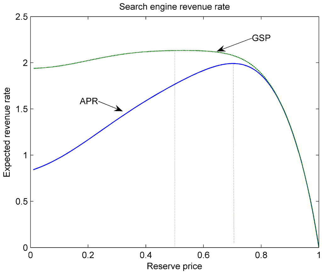
Figure 1. Search engine’s expected revenue rates from APR and GSP mechanisms

Figure 1. Search engine’s expected revenue rates from APR and GSP mechanisms

Figure 1 depicts the search engine’s expected revenue rates versus reserve price in APR and GSP, respectively. GSP creates more revenue than APR, and its revenue advantage disappears as the reserve price increases. It is clear that the optimal reserve price in GSP is 0.5 according to (15). Figure 1 also verifies that the search engine should set the reserve price higher in APR.

4.3. Advertiser Population

Each keyword for sale has its own market, whose demand is gauged by both the market size and depth. While market size represents the average number of potential buyers, market depth stands for the amount they each bid. The dynamic nature of advertising business is likely to influence the market size and depth over the course of time. Hence, it is necessary for the search engine to review the reserve price for each keyword when such changes in the market take place. The following proposition shows how the population of potential bidders affects the optimal reserve price.

Corollary 3 In APR where the value distribution is IGFR, the optimal reserve price r is an increasing function of the arrival rate of advertisers λ.

Any additional demand is beneficial to the search engine because a new advertiser not only pays more for a sponsored link than the current reserve price, but also increases the competition and prompts other advertisers to raise the bids accordingly to secure their positions. Hence, given the limited space for displaying sponsored results on its front page, when the population of bidders for a keyword increases, the search engine should lift reserve price to create more revenue. Recognizing the importance of the market size, search engines make continuous efforts to recruit new advertisers. For instance, Yahoo! offers a $25 of signing credit for any new customer. In addition, no longer using the fixed $.10 minimum bid policy for sponsored search, Yahoo! now adjusts reserve price in a particular keyword market based on multiple factors including the number of bidders and the bid amounts (see Yahoo! Search Marketing Help [17]). Such a shift in pricing strategy corroborates our theoretical findings.

5. Conclusion

In sponsored search advertising advertisers compete for ad links that appear in the front page of major search engines including Google and Yahoo! through auctions. Search engines often set variable reserve price to influence advertiser’s bidding and create more revenue. However, as advertising capacity is perishable, arbitrary thresholds may adversely affect revenues.

This paper compares two pricing mechanisms in sponsored search advertising—the generalized second-price auction (GSP) where the last winning position is charged the larger value between the reserve price and the highest losing bid, and an alternative GSP with posted reserve price (APR) where the last winning position pays the reserve price regardless how many positions are sold. Although the standard GSP is extensively studied in the literature to derive optimal reserve price, it fails to capture the dynamics of the auction. The continuous bidding game is unlikely to have the same number of unsold positions in each period and may require periodical reviews of the reserve price. The proposed APR mechanism is an attempt to remedy the problem. We assume that the number of eligible bidders is endogenously controlled by the reserve price. Focusing on the lower bound of the SNE our models maximize the long-term expected revenue rate. If the value per click of bidders has the property of IGFR, the expected revenue rates in both GSP and APR are quasi-concave of the reserve price and there exists a unique optimizer for each mechanism. In particular, the optimal reserve price in GSP is proved to be the same as the one in single-item auctions that is dependent on only the private value distribution. In contrast, the optimal reserve price in APR, depending on both the numbers of bidders and positions, should be set higher compared with the one in GSP.

Current research can be extended in several directions. First, in our model the CTR of each slot is exogenous. Although this is a standard assumption, it may not always be the case especially when not all slots are occupied. For instance, when it is only ad showing the link on the right of the first page may receive more clicks than when it has companies. Taking this situation into account will make our pricing model much more complex. On the other hand, it may facilitate the analysis on the optimal number of sponsored links a search engine should sell in the first page. Second, our model maximizes the expected revenue rate in a static auction with an endogenous number of bidders. It might be interesting to consider a dynamic model investigating how the search engine should update the reserve price at each period based on the incumbent and potential new entry. Third, it is worth exploring the Bayes–Nash equilibria of GSP and APR, and investigating whether the Revenue Equivalence Theorem (Myerson [9]) applies to the two mechanisms.

References

- Google Inc. 2011 Annual Report on Form 10-K. Available online: http://www.sec.gov/Archives/edgar/data/1288776/000119312512025336/d260164d10k.htm (accessed on 1 April 2012).
- Brooks, N. The Atlas Rank Report: How Advertisement Engine Rank Impacts Traffic; Technical Report; Atlas Institute, University of Colorado: Boulder, CO, USA, July 2004. [Google Scholar]
- Yahoo! Search Marketing Blog. Reserve Prices, Minimum Bids No Longer Fixed at $.10 for Sponsored Search. Available online: http://www.ysmblog.com/blog/2008/02/26/minimum-bids/ (accessed on 1 February 2009).
- Google Adwords Help. What Ad Position Is the First Page Bid Related to? Available online: http://adwords.google.com/support/bin/answer.py?hl=en&answer=104241 (accessed on 12 February 2011).
- Google Adwords Help. How Much Do I Pay for a Click on My Ad? What If My Ad Is the Only One Showing? Available online: http://adwords.google.com/support/bin/answer.py?hl=en&answer=87411 (accessed on 12 February 2011).
- Edelman, B.; Ostrovsky, M.; Schwarz, M. Internet advertising and the generalized second price auction: Selling billions of dollars worth of keywords. Am. Econ. Rev. 2007, 97(1), 242–259. [Google Scholar] [CrossRef]
- Varian, H.R. Position auctions. Int. J. Ind. Organ. 2007, 25(6), 1163–1178. [Google Scholar] [CrossRef]
- Yang, W.; Feng, Y.; Xiao, B. Dynamic reserve price in sponsored search advertising. LIU Post, 2012; (working paper). [Google Scholar]
- Myerson, R.B. Optimal auction design. Math. Oper. Res. 1981, 6(1), 58–73. [Google Scholar] [CrossRef]
- Riley, J.G.; Samuelson, W.F. Optimal auctions. Am. Econ. Rev. 1981, 71(3), 381–392. [Google Scholar]
- Maskin, E.; Riley, J. Optimal Multi-Unit Auctions; Oxford University Press: Oxford, UK, 1989. [Google Scholar]
- Bulow, J.; Roberts, J. The simple economics of optimal auctions. J. Polit. Econ. 1989, 97(5), 1060–1090. [Google Scholar] [CrossRef]
- Edelman, B.; Schwarz, M. Optimal auction design and equilibrium selection in sponsored search auctions. Am. Econ. Rev. 2010, 100(2), 597–602. [Google Scholar] [CrossRef]
- Xiao, B.; Yang, W. A revenue management model for products with two capacity dimensions. Eur. J. Oper. Res. 2010, 205(2), 412–421. [Google Scholar] [CrossRef]
- Feng, Y.; Xiao, B. A continuous-time yield management model with multiple prices and reversible price changes. Manage. Sci. 2000, 46(5), 644–657. [Google Scholar] [CrossRef]
- Wang, R. Auctions versus posted-price selling. Am. Econ. Rev. 1983, 83(4), 838–851. [Google Scholar]
- Yahoo! Search Marketing Help. Pricing and Minimum Bids. Available online: http://help.yahoo.com/l/us/yahoo/ysm/sps/faqs_all/faqs.html#pricing (accessed on 1 May 2009).
- Harris, M.; Raviv, A. A theory of monopoly pricing schemes with demand uncertainty. Am. Econ. Rev. 1981, 71(3), 347–365. [Google Scholar]
- Wilson, R.B. Nonlinear Pricing; Oxford University Press: Oxford, UK, 1993. [Google Scholar]
- Roth, A.; Sotomayor, M. Two-Sided Matching; Cambridge University Press: Cambridge, UK, 1990. [Google Scholar]
- Lariviere, M.A.; Porteus, E.L. Selling to the newsvendor: An analysis of price-only contracts. M&SOM-Manuf. Serv. Op. 2001, 3(4), 293–305. [Google Scholar]
- Ziya, S.; Ayhan, H.; Foley, R.D. Relationships among three assumptions in revenue management. Oper. Res. 2004, 52(5), 804–809. [Google Scholar] [CrossRef]
- Lariviere, M.A. A note on probability distributions with increasing generalized failure rates. Oper. Res. 2006, 54(3), 602–604. [Google Scholar] [CrossRef]
© 2013 by the authors; licensee MDPI, Basel, Switzerland. This article is an open access article distributed under the terms and conditions of the Creative Commons Attribution license (http://creativecommons.org/licenses/by/3.0/).