Bounded Memory, Inertia, Sampling and Weighting Model for Market Entry Games

Abstract
: This paper describes the “Bounded Memory, Inertia, Sampling and Weighting” (BI-SAW) model, which won the http://sites.google.com/site/gpredcomp/Market Entry Prediction Competition in 2010. The BI-SAW model refines the I-SAW Model (Erev et al. [1]) by adding the assumption of limited memory span. In particular, we assume when players draw a small sample to weight against the average payoff of all past experience, they can only recall 6 trials of past experience. On the other hand, we keep all other key features of the I-SAW model: (1) Reliance on a small sample of past experiences, (2) Strong inertia and recency effects, and (3) Surprise triggers change. We estimate this model using the first set of experimental results run by the competition organizers, and use it to predict results of a second set of similar experiments later ran by the organizers. We find significant improvement in out-of-sample predictability (against the I-SAW model) in terms of smaller mean normalized MSD, and such result is robust to resampling the predicted game set and reversing the role of the sets of experimental results. Our model's performance is the best among all the participants.1. Introduction
Studying and modeling human learning behavior in the laboratory has always been an important research topic in economics (See Chapter 6 of Camerer [2] for a review). For example, Erev and Roth [3] consider reinforcement models, while Camerer and Ho [4] consider a hybrid model of belief-based and reinforcement learning. However, recent articles had shown that experimental environment variation and relatively small datasets and models had brought difficulties into the literature (see, for example, Salmon [5]). Different experimental environment and setting may lead to learning behavior worlds apart. Most previous studies focused on relative small datasets, therefore making it difficult to obtain a general model. Erev et al. organized a model estimation contest in 2009, attempting to solve this using a large dataset and uniform experimental setups. Results were reported in Erev et al. [6]. However, their setup considered only the environmental uncertainty individuals face and restricts payoff feedbacks to obtained payoff. In other words, subjects do not know what their forgone payoffs are.
Erev et al. [1] further held a second prediction competition to investigate model variation on the addition of uncertainty due to information asymmetries and information on forgone payoff. This competition is based on the market entry game, which is a binary choice game where players face a safe choice and a risky option. Both choices include environmental uncertainty, but the payoff of the risky choice will be affected by other players. The payoffs of the chosen and forgone options were both shown to the subjects in this competition.
The competition organizers ran experiments to generate two sets of experimental data, the estimation game set and the competition game set. Seeing the experimental results of the estimation game set, participants of the competition are asked to predict the behavior of the competition game set when only several given game parameters were known, but not the actual responses of the experimental subjects.
Based on the results of the previous competition, Erev et al. [1] introduced the best baseline model called the inertia, sampling and weighting (I-SAW) model. The I-SAW model consists of three different modes, exploration, exploitation and inertia mode. A player in the exploration mode would enter randomly with a fixed probability that varies across subjects. In the market entry game, exploration mode is the resemblance of decision without experience. Under the exploitation mode, subjects make decision based on past experiences. Specifically, subjects form the Estimate Subjective Value (ESV) by calculating a weighted average between the sample mean of a small sample of past history and the grand mean of all past experience. The Inertia mode signifies the personal beliefs of players. In this mode, players act the same as the immediate past. The probability of entering the exploration mode is fixed among subjects, whereas the probability of entering the inertia mode is decided by past experiences, the more surprise a payoff is, the less one will enter the inertia mode. If a player does not enter either the exploration or the inertia mode, she will enter the exploitation mode. Each player has some underlying parameters to reflect individual differences, which is drawn from a population distribution.
However, we believe that the “perfect recall” assumption in the exploitation mode is not realistic. Specifically, the exploitation mode says that while sampling from the past, all past periods are considered regardless of the size of gap between now and a certain past. As Simon [7] first proposed, “global rationality” may not be “…actually possessed by organisms, including man, in the kinds of environments in which such organisms exist.” The assumption of memory retrieval to the unlimited past is not solid on human being.
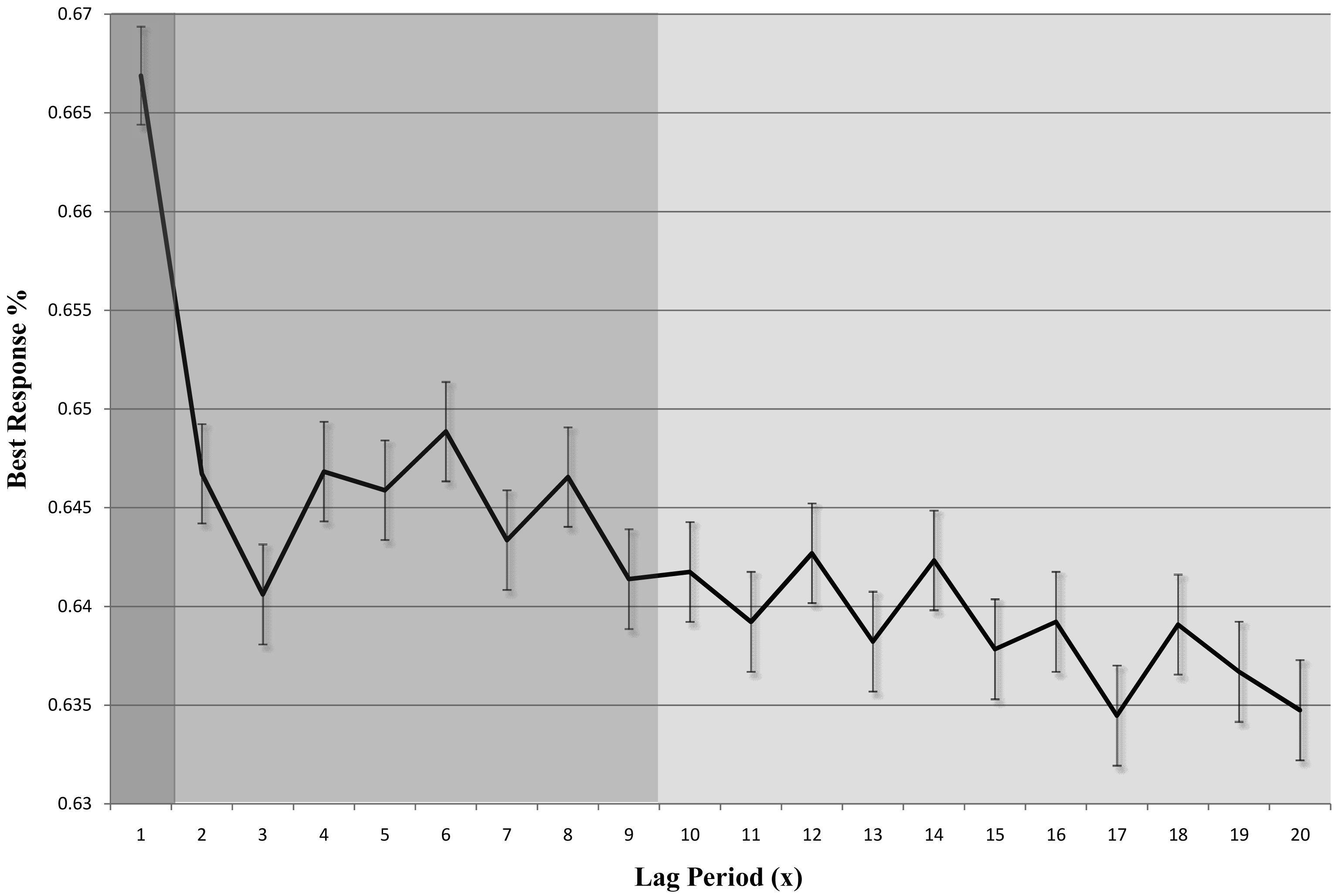
In fact, we find that the participants tend to choose the best response in the recent periods. Specifically, we calculate the percentages of choice in the current period (t) that coincide with the best response in a previous period (t − x), and present it in Figure 1. As shown in the figure with different colors, there are three levels of best response percentage (1, 2 to 9, and 10 to 20). This difference proves our suspicion toward “perfect recall”.1 2
Therefore, we introduce the concept of bounded memory into the I-SAW model to avoid this unlimited reminiscence problem. In particular, players will be able to recall exact payoffs only from some near past, though they should be able to have some vague idea or feelings about a general past of a choice. Hence, we set the sample mean to be sampled from some near past rather than sampling from all history, while maintaining the I-SAW assumption that the grand mean is the average of all past experiences. This modification captures the intuition that an elder may know that her birthday has been great all her life, but it is rare for an old lady to tell about what she got on her twelfth birthday, even though her recollection of last year's birthday present may be precise.
We estimate the modified model of Bounded memory, Inertia, Sampling and Weighting (BI-SAW) by grid search. The grid search method seeks the best fit parameter set under a particular chosen criterion and data. The criterion we utilize is exactly the one used in the prediction competition, the average of six normalized mean square deviations. This criterion focuses on the model's prediction ability in terms of game entry rate, efficiency rate and alternation rate. We estimated the BI-SAW model by using experimental data of the estimation game set provided by the competition organizers. For each parameter set of interest we perform ten thousand simulations of the estimation game set. This number was chosen to be large enough to eliminate the effect of randomness inherent in the BI-SAW population model which draws a set of parameters for each individual. We follow Erev et al. [1] and model this set of individual parameters as independent and identical draws from a uniform distribution with lower bounds of zero (one for discrete parameters), and upper bounds set as population parameters of the model.3 On the other hand, though also estimated from data, we specified the memory limitation to be constant among all players for simplicity.
In the prediction competition, the BI-SAW model with a bounded memory limitation of 6 periods predicts data of the competition game set better than the benchmark I-SAW model, as well as other models submitted by 13 groups of contestants.4 Due to the random nature of the competition, we perform three tests concerning the randomness of outcome, game set selection, and parameter estimation game set. All three results favor the BI-SAW model. In particular, the BI-SAW model significantly outperforms the benchmark I-SAW model in repeated simulations of the outcome. Also, the BI-SAW model predicts significantly better than the I-SAW model even when the prediction target is a resample of the competition game set. Thirdly, the BI-SAW model still performs better than the I-SAW model even after we reverse the role of the estimation and competition game sets. To sum up, the BI-SAW model is precise and robust in the market entry game.
The remaining of the article is organized as follows: Section 2 describes the BI-SAW model, Section 3 describes the market entry game designed for the prediction competition, Section 4 presents our estimation method, Section 5 presents the results, and Section 6 concludes.
2. The BI-SAW Model
The Bounded Memory, Inertia, Sampling and Weighted (BI-SAW) model is a type of explorative sampler model that features strong inertia, recency effects, surprise triggers change, and a restriction on individual's ability of recalling past payoffs when sampling. To be specific, the BI-SAW model dictates that in every trial each individual enters one of the 3 response modes (Exploration, Exploitation or Inertia) based on randomness and her past experience such as surprise. The probability of choosing a specific action under each mode is then determined by specific predetermined rules that are also based on past experiences and randomness. The idea is that people would enter different mindsets when facing different payoff histories and the same histories will also determine the action people choose in each mindset.
2.1. Three Response Modes
Individual i (= 1,…, n) enters the exploration mode with probability 1 in the first trial, and ∊i (a trait of i) in all other trials. In this mode, the individual chooses her action according to an exogenous distribution P0. For instance, if the individual faces a binary choice of 0 or 1 and P0 = (p0, 1 − p0), she would choose 0 with probability p0, and choose 1 with probability (1 − p0). Notice that P0 is homogeneous across individuals.
2.2. Inertia Mode
If the exploration mode was not chosen, individual i enters the inertia mode at trials (t + 1) with probability πi to the power of Surprise(t), , where πi ∈ [0,1] is the lowest probability of entering the inertia mode (when there is maximum surprise), and Surprise(t) ∈ [0,1] is the surprise individual i feels after receiving the payoff of trial t. This reflects how individuals stick to “business-as-usual” unless they encounter a big shock in their life (surprise).
To define this surprise, we shall first define the payoffs gap with respect to GrandMj(t), the average payoff from choosing action j (= 1,…, k) in all the previous trials. The payoff gap, Gap(t), is the average difference between payoffs received (or forgone) from choosing each action in trial t and (t − 1), and between trial t and the average payoff from choosing that action:
The running average of the payoff gap is:
Based on Gap(t) and Mean_Gap(t), we can now define the surprise at trial t:
Since πi ranges from 0 to 1, less surprise will trigger more inertia, and vice versa. Also, notice that the Surprise(t) is normalized to between 0 and 1, thus the probability of inertia is between πi and 1.
2.3. Exploitation Mode
If neither the exploration mode nor the inertia mode were chosen, an individual will enter the exploitation mode. To be specific, the probability of entering this mode is 0 in the first trial, and in all other trials is 5
Under this mode, individual i first calculates the Estimated Subjective Value (ESV) for each action, in the trial t (> 1), and chooses the action with the highest ESV:
2.4. Interpreting BI-SAW
We summarize our parameters and their interpretations as follow
∈i is the chance of entering the exploration mode starting from the second trial. Since we assume, under this mode, people all choose their actions according to a fixed distribution independent of experience, this parameter can be interpreted as people's tendency to explore different possibilities. In our setting (the market entry game), since we assume individuals would choose the risky choice with high probabilities in the exploration ode, this also implies the tendency to take risk.
P0 is the distribution of actions an individual follows when entering the exploration mode, and is the same for all individuals.
πi is the lower bound for the probability of entering the inertia mode starting from the third trial. Higher πi means a higher possibility for the individual to repeat her last choice, and also a lower probability for entering the exploitation mode. When πi = 1, unless the exploration mode was chosen, individual will stick to her last choice starting from the third trial.
wi measures the weight placed on the grand average payoff of all past experiences, instead of the small sample average payoff. Higher wi suggests that individual i puts more weight on the grand average, rather than relying on the small sample average. When wi = 1, for example, the individual will simply choose the action which gives her the highest grand average payoff.
ρi measures the tendency to select the most recent trial when sampling. Higher ρi suggests that the payoff from the most recent trial will have a bigger impact on the individual. When ρi = 1 and wi = 0, individual will consider only the most recent trial when conducting the small-size sampling in the exploitation mode.
µi is the number of trials an individual samples when she calculates the small sample average. Higher µi implies more trials of experiences were considered when making decisions. When µi = ∞ and ρi = 0, the small sample average will converge to the grand average payoff.
b measures individual's ability of recalling past payoffs in terms of the number of trials. Thus, higher b naturally implies a better working memory, or a better technique for memorizing payoffs. Since previous literature (Miller [8]) reports a memory capacity of 5 to 6 chunks with a small variance among individuals, we assume all individuals have the same b, instead of allowing them to have different bi.
2.5. From Individual Model to Population Prediction
We have thus defined an individual BI-SAW model where each individual is represented by a parameter vector (∈i, P0, πi, wi, ρi, µi, b). To form a population prediction, we draw each individual parameter from a uniform distribution with a fixed lower bound.6 For the population model, we estimate the upper bounds for the 5 individual parameters and b. We do not estimate P0, but use the average initial entry rate in the data instead. We then generate our outcome prediction by simulating 5000 times and take the average.
3. The Market Entry Game
The market entry game we study in this paper exhibits environmental and strategic uncertainty in which four players each face a binary choice in each trial: entering a risky market or staying out (a safe prospect). After making their choices, each player will receive feedback including the payoff they just earned and the payoff they would have earned had they chosen the alternative.
The payoff of entering the risky market (V(t)) will depend on the number of entering players (E) and the realization of a binary gamble Gt:
The probability that H will be realized in a trial is given by:
The payoff of staying out depends on Gt and a safety parameter s(> 1), which equals to Gt/s or −Gt/s, round to the nearest integer, with equal probability. Therefore, the expected payoff of staying out equals to zero and its variance is smaller than that of the entering payoff.
Notice that the exact payoff structure described above is unknown to players. What they know is: their payoff in each trial depends on “their choices, the state of nature and on the choices of the other participants (such that the more people enter the less is the payoff from entry).” (Erev et al. [1])
Although parameters are the same in a game, Gt and E may vary from trial to trial in the same game, serving as environmental and strategic uncertainty in the market respectively.
This market entry game is a stylized representation of a common economic problem: the utility of undertaking a particular activity depends on the environment, and decreases as the number of participants increases. For example, when choosing to go to the amusement park, one's utility depends on not only the weather, but also how many visitors there are. Therefore, both environmental and strategic uncertainty are taken into consideration when making decisions.
4. Estimation Methodology
The competition organizers randomly draw 40 sets of game parameters (k, H, L, s) to form the estimation game set, and conduct experimental sessions that run 50 trials for each game. They then randomly draw another 40 sets of game parameters from the same class of market entry games to form the competition game set, and then conduct experiments that also run 50 trials for each game. Experimental subjects were recycled to participate in several different games, but the exact subset of games subjects participated were not revealed, so we can only treat players of each game as independent.
The prediction competition uses mean normalized mean square deviation (MNMSD) scores as the criterion when comparing predictions of different models. This mean normalized MSD score is the average of mean square deviations (MSD) between experimental data and model prediction in three aspects: entry rate, efficiency level and alternation rate. Therefore, we need three MSDs to calculate the MNMSD score: entry MSD, efficiency MSD, and alternation MSD. Moreover, we divide each game's data into two blocks, block 1 (trials 1-25) and block 2 (trials 26-50), and calculate the three MSDs for each block. To obtain the MNMSD score of a certain model's prediction, we calculate the entry, efficiency and alternation MSD for block 1 and 2, normalize these six numbers to make them comparable, and take the average.8
Here, the entry MSD for a certain model (in a given block of a particular game) is the squared difference of the predicted and actual entry rate (frequency of entry divided by the total number of decisions in the block). We then derive the overall entry MSD by taking the average of the entry MSD in every game. The alternation MSD is similarly defined. Thirdly, we calculate the efficiency MSD of each game by dividing total decision gain by total number of decisions, and average across games.
We do not estimate the probability of entering under exploration mode (p0). Instead, we set it equals to the average entry rate in all first trials of the estimation game set.
On the other hand, we estimate the population BI-SAW model through grid search to look for the best upper bounds: ∈̅, w̅, ρ̅, π̅, µ̅, (for the distribution of individual parameters) and b that minimizes MNMSD of a given set of games. Based on the best fit of the I-SAW model (Erev et al. [1]), we choose an initial range listed in Table 1. Since MSD varies for the population model (due to sampling of individual parameters), we simulate the outcome 10,000 times for each set of parameters, and choose the set that minimizes the average MNMSD for these 10,000 times.9
5. Empirical Results
We first report the results of our estimation and model fit, and then discuss the significance of the bounded memory assumption.
5.1. Basic Estimation and Model Fit
To obtain the 6 normalized MSD scores, we use the parameters estimated using the estimation game set, and simulate the experimental results of the competition game set for 5000 times. We then take the average of the 5000 simulation results, and normalize them.
Table 2 reports the 6 normalized MSD scores of the BI-SAW model (entry MSD, efficiency MSD, and alternation MSD for each of the two blocks), and compares them with those of the I-SAW model (the best baseline model reported in Erev et al. [1]) when both models are estimated using the estimation game set. The BI-SAW model's 6 normalized MSD scores are all smaller than those of the I-SAW model, for the estimation game set, especially for the entry MSD and the efficiency MSD of block 1. The MNMSD score of the BI-SAW model is 1.2454 and the MNMSD score of the I-SAW model is 1.3674. Hence, the BI-SAW model has a better in-sample fit than the best baseline model in the literature (the I-SAW model).
Moreover, the BI-SAW model outperforms the I-SAW model in predicting out-of-sample data (the competition game set). Table 2 also reports the 6 normalized MSD scores of the BI-SAW and I-SAW model for the competition game set. We can see that the BI-SAW model's normalized MSD scores are always smaller than the I-SAW model's normalized MSD scores except for the alternation MSD of block 2 (0.8979 vs. 0.8571). The MNMSD score of the BI-SAW model is 1.0151, and the MNMSD score of the I-SAW model is 1.1742. This result provides strong evidence that the BI-SAW model predicts new experimental results better than the I-SAW model.
5.2. The Significance of the Bounded Memory Assumption
Since MNMSD is an abstract number, we use the following three ways to test the significance of the bounded memory assumption, which is the only difference between the BI-SAW and I-SAW model: outcome simulation on the competition game set, prediction on resampled game sets, and reversing the role of the estimation and competition game sets.
5.3. Outcome Simulation on the Competition Game Set
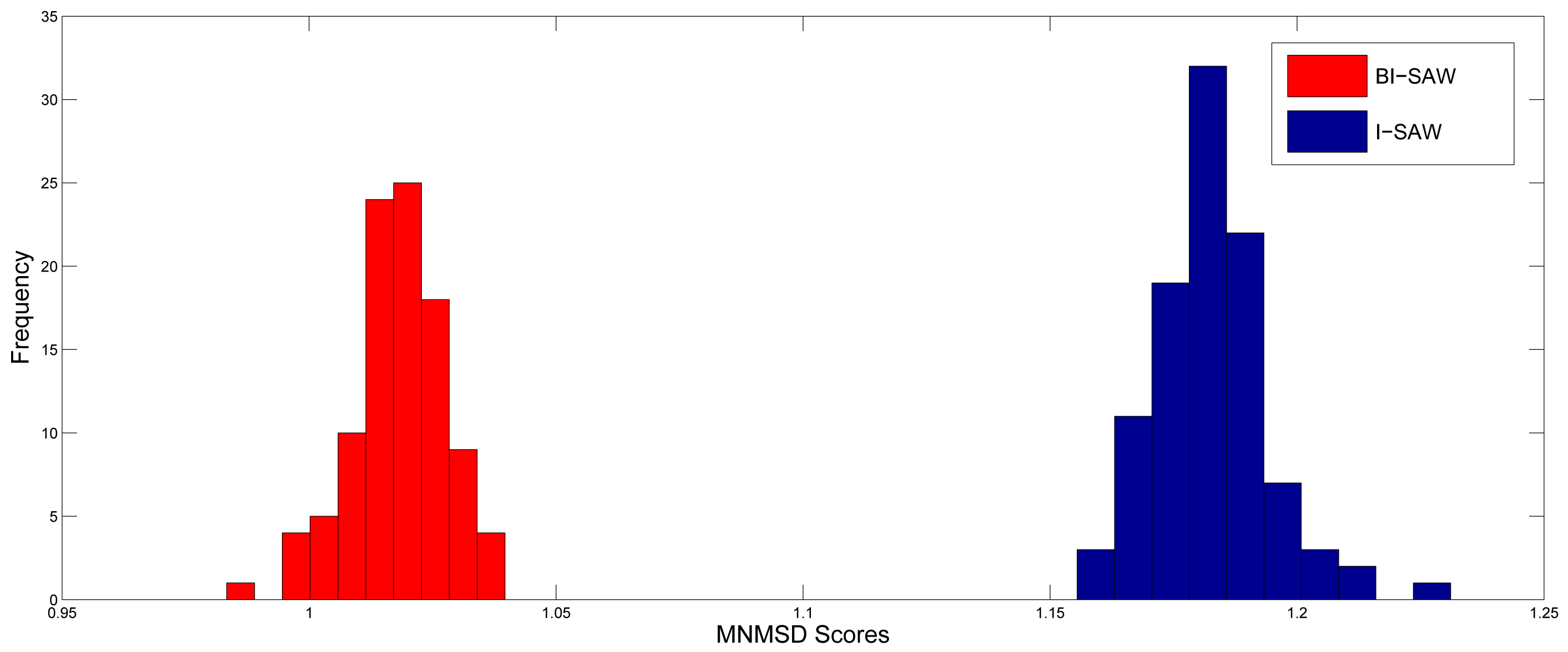
There is randomness in the 6 normalized MSD scores due to outcome simulation, so we have to make sure the BI-SAW model performs better not only because of this randomness. For this purpose, we repeat the simulation procedure described in Section 5.1 for 100 times. Figure 2 shows the distributions of MNMSD scores for both models. It is clear that the MNMSD scores of the BI-SAW model are always smaller than those of the I-SAW model. Results of the Wilcoxon signed-rank test and the paired t-test are both significant with p-value = 0.000. 10
5.4. Prediction on Resampled Game Sets
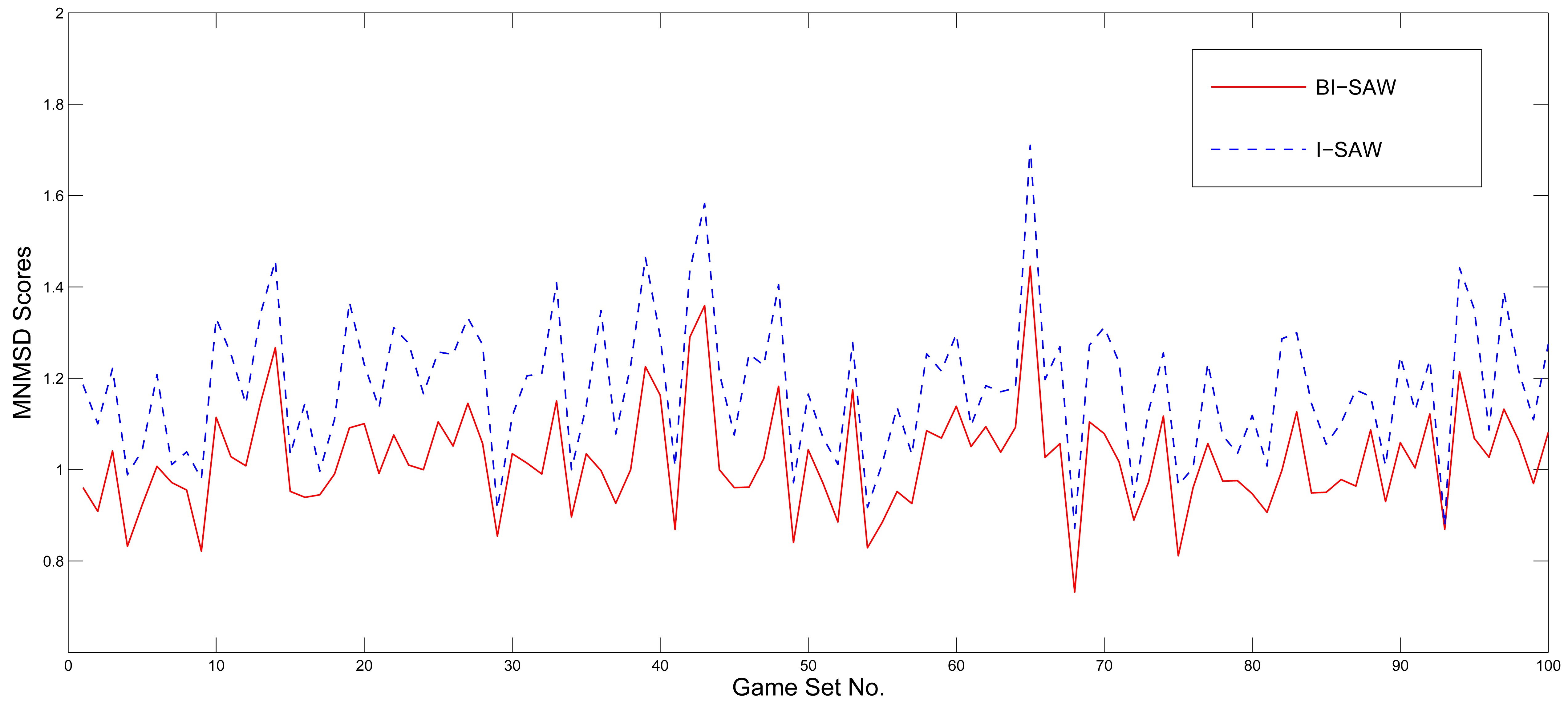
To test whether the BI-SAW model's prediction power is robust to different game sets, we draw 40 games with replacement from the competition game set to form a new game set, and see if our estimated BI-SAW model still predicts well in the new game set. This resampling procedure is justified by the fact that the parameters of each game in both the estimation and competition game sets were also randomly drawn by the organizers of the competition. We repeat the resampling process for 100 times and use both the I-SAW and BI-SAW model to simulate results of these 100 resampled game sets. Figure 3 shows the MNMSD scores of the 100 resampled game sets of both models. The MNMSD scores of the BI-SAW model are never larger than those of the I-SAW model in all resampled game sets. Consequently, the results of the Wilcoxon signed-rank test and paired t-test are both significant with p-value = 0.000.
5.5. Reversing the Role of Estimation and Competition Game Sets
Finally, to test whether our estimated BI-SAW model predicts well only in the estimation game set, we reverse the roles of the estimation and competition game sets. That is, we estimate the parameters using the original competition game set, and use it to predict the results of the original estimation game set. In other words, the original competition game set is now viewed as in-sample data, and the original estimation game set is now viewed as out-of-sample data. Table 2 reports the 6 new normalized MSD scores of the I-SAW and BI-SAW model. Note that the parameters are now estimated from the (original) competition game set. The estimated parameters of the I-SAW and BI-SAW model differ largely from the original ones. The MNMSD score of the I-SAW model is even smaller than that of the BI-SAW model for the original competition game set (now in-sample data). Notwithstanding, the BI-SAW model still outperforms the I-SAW model out of sample. In particular, the MNMSD score of the BI-SAW model, 1.6092, is still smaller than the MNMSD score of the I-SAW model, which is 1.6232.
6. Conclusions
In this paper, we propose the “Bounded Memory, Inertia, Sampling and Weighted (BI-SAW)” model in which the subjects' ability of recalling past experience is assumed to be limited. This assumption is crucial when modeling how people make decisions based on their past experience. We test if it improves models' prediction power in a market entry game setting with strategic and environmental uncertainty, in which each player receives feedback regarding earned and forgone payoffs after each decision.
To evaluate the significance of the bounded memory assumption, we verify that the prediction power of the BI-SAW model is consistently stronger than the benchmark I-SAW model by comparing model performance using the mean normalized mean square deviation (MNMSD) criterion in the following three settings. First of all, we repeatedly simulate the outcome of the two models for the competition game set for 100 times to see if the difference between MNMSD scores is significant. Secondly, we use 100 resampled game sets (by repeatedly drawing 40 new games from the competition game set) to check whether the prediction power of BI-SAW model is independent of game sets. Thirdly, we reverse the role of the estimation game set and the competition game set, and perform the same estimation-and-prediction exercise. In all three cases, the BI-SAW model outperforms the I-SAW model, by having lower out-of-sample MNMSD scores. These results confirm the robustness of the BI-SAW model performance. Thus, by incorporating the bounded memory assumption, the BI-SAW model integrates realistic limitations of the human brain into economic modeling, and commands a better ability in predicting subjects' choices.
There are still several open questions to be resolved in future work. The most obvious one is to generalize the BI-SAW model to cope with different information settings. For instance, it would be interesting to see if the BI-SAW model also outperform the I-SAW model in games in which forgone payoffs are unknown (such as those reported in Erev et al. [6]).
Another area that deserves further investigation is exploring other possible specifications and extensions of the bounded memory assumption. In particular, we assume that all subjects recall payoffs of the last b trials. One could use other criteria to determine which memory are recalled, such as frequency of encountering the same situation, etc. Adding such extension should create a better way to predict how people play games in experimental setting, and eventually how they make decisions in daily life.


| Parameters | Estimation Range | Precisions |
|---|---|---|
| ε̅ | [0.1,0.4] | 0.01 |
| w̅ | [0,1] | 0.1 |
| ρ̅ | [0,1] | 0.1 |
| π̅ | [0,1] | 0.1 |
| µ̅ | [1,5] | 1 |
| b | [1,25] | 1 |
| Model | I-SAW | BI-SAW | I-SAW | BI-SAW |
|---|---|---|---|---|
| Estimated with | Estimation game set | Competition game set | ||
| Entry Rate normalized MSD (block 1) | 1.5443 | 1.2763 | 1.1627 | 1.1510 |
| Entry Rate normalized MSD (block 2) | 1.1495 | 1.1500 | 0.8621 | 0.8357 |
| Efficiency normalized MSD (block 1) | 1.3106 | 1.0746 | 0.7105 | 0.7352 |
| Efficiency normalized MSD (block 2) | 1.4899 | 1.3454 | 0.8218 | 0.8818 |
| Alternation normalized MSD (block 1) | 1.4192 | 1.3802 | 0.7130 | 0.7118 |
| Alternation normalized MSD (block 2) | 1.2913 | 1.2456 | 0.7437 | 0.8382 |
| In-sample MNMSD | 1.3674 | 1.2454 | 0.8356 | 0.8589 |
| Prediction on | Competition game set | Estimation game set | ||
| Entry Rate normalized MSD (block 1) | 1.7353 | 1.4009 | 1.6043 | 1.6133 |
| Entry Rate normalized MSD (block 2) | 1.6431 | 1.3385 | 1.6608 | 1.6811 |
| Efficiency normalized MSD (block 1) | 0.8878 | 0.7650 | 1.0480 | 1.0334 |
| Efficiency normalized MSD (block 2) | 1.1714 | 1.0078 | 2.1256 | 2.1659 |
| Alternation normalized MSD (block 1) | 0.7507 | 0.6808 | 1.8640 | 1.7951 |
| Alternation normalized MSD (block 2) | 0.8571 | 0.8979 | 1.4367 | 1.3666 |
| Out-of-sample MNMSD | 1.1742 | 1.0151 | 1.6232 | 1.6092 |
| Estimated Parameters | ||||
| ∈̅ | 0.24 | 0.25 | 0.20 | 0.20 |
| w̅ | 0.8 | 0.8 | 0.6 | 0.6 |
| ρ̅ | 0.2 | 0.8 | 1.0 | 1.0 |
| π̅ | 0.6 | 0.6 | 0.6 | 0.6 |
| μ̅ | 3 | 3 | 2 | 2 |
| b | - | 6 | - | 8 |
Acknowledgments
We are grateful to Joseph Tao-yi Wang for his encouragement, support and advice. We thank the suggestion of two referees, Yi-Ching Lee, the audience of the 2010 North American Meeting of the Economic Science Association. We acknowledge support from the Taiwan Social Science Experimental Laboratory of National Taiwan University and the NSC of Taiwan (NSC 98-2410-H-002-069-MY2, NSC 99-2410-H-002-060-MY3).
References
- Erev, I.; Ert, E.; Roth, A.E. A choice prediction competition for market entry games: An introduction. Games 2010, 1, 117–136. [Google Scholar]
- Camerer, C.F. Behavioral Game Theory: Experiments on Strategic Interaction; Princeton University Press: Princeton, NJ, USA, 2003. [Google Scholar]
- Erev, I.; Roth, A.E. Predicting how people play games: Reinforcement learning in experimental games with unique, mixed strategy equilibria. Amer. Econ. Rev. 1998, 88, 848–881. [Google Scholar]
- Camerer, C.; Ho, T.H. Experience-weighted attraction learning in normal form games. Econometrica 1999, 67, 827–874. [Google Scholar]
- Salmon, T.C. An evaluation of econometric models of adaptive learning. Econometrica 2001, 69, 1597–1628. [Google Scholar]
- Erev, I.; Ert, E.; Roth, A.E.; Haruvy, E.; Herzog, S.M.; Hau, R.; Hertwig, R.; Stewart, T.; West, R.; Lebiere, C. A choice prediction competition: Choices from experience and from description. J. Behav. Decis. Making 2010, 23, 15–47. [Google Scholar]
- Simon, H.A. A behavioral model of rational choice. Quart. J. Econ. 1955, 69, 99–118. [Google Scholar]
- Miller, G. The magical number seven, plus or minus two: Some limits on our capacity for processing information. Psychol. Rev. 1956, 63, 81–97. [Google Scholar]
- 1We use the data from the estimation game set.
- 2In order to observe a large range of lags (x) up to 20, only periods (t) 21 to 50 are included. Also note that our result is different from the one shown in Erev et al. [1] because they use periods 13 to 50.
- 3The uniformly distributed individual parameters and their implications can be reviewed in Erev et al. [1].
- 4Even if we use a bounded memory limitation of 7 periods, the BI-SAW model still outperforms all other models.
- 5Notice that, as we saw in the inertia mode, is not dened in the second trial. Therefore, in trial 2, individual i can only enter either the exploration mode or the exploitation mode.
- 6Except for b and P0, which are the same for all individuals.
- 7E(Gt) = PH * H + (1 – PH)* L = [–L/(H – L)] *H + [H/(H – L) ] * L = 0.
- 8See Erev et al. [1] for details.
- 9Reduce this sampling error is important as the MNMSD of competing models differ only by ±0.05 (Figure 2).
- 10If b is allowed to have individual differences, and drawn from a normal distribution with mean 6 and s.d. 2.5 (truncated below 0), the MNMSD scores could be reduced to 0.9832. (We estimate the s.d. by using the estimation game set.) Moreover, a similar horse race reveals that this modified version outperforms the original BI-SAW model. Results of the Wilcoxon signed-rank test and the paired t-test are both significant with p-value = 0.000.
© 2011 by the authors; licensee MDPI, Basel, Switzerland. This article is an open access article distributed under the terms and conditions of the Creative Commons Attribution license (http://creativecommons.org/licenses/by/3.0/.)
Share and Cite
Chen, W.; Liu, S.-Y.; Chen, C.-H.; Lee, Y.-S. Bounded Memory, Inertia, Sampling and Weighting Model for Market Entry Games. Games 2011, 2, 187-199. https://doi.org/10.3390/g2010187
Chen W, Liu S-Y, Chen C-H, Lee Y-S. Bounded Memory, Inertia, Sampling and Weighting Model for Market Entry Games. Games. 2011; 2(1):187-199. https://doi.org/10.3390/g2010187
Chicago/Turabian StyleChen, Wei, Shu-Yu Liu, Chih-Han Chen, and Yi-Shan Lee. 2011. "Bounded Memory, Inertia, Sampling and Weighting Model for Market Entry Games" Games 2, no. 1: 187-199. https://doi.org/10.3390/g2010187