Adaptive Covariance Estimation Method for LiDAR-Aided Multi-Sensor Integrated Navigation Systems

Abstract

The accurate estimation of measurements covariance is a fundamental problem in sensors fusion algorithms and is crucial for the proper operation of filtering algorithms. This paper provides an innovative solution for this problem and realizes the proposed solution on a 2D indoor navigation system for unmanned ground vehicles (UGVs) that fuses measurements from a MEMS-grade gyroscope, speed measurements and a light detection and ranging (LiDAR) sensor. A computationally efficient weighted line extraction method is introduced, where the LiDAR intensity measurements are used, such that the random range errors and systematic errors due to surface reflectivity in LiDAR measurements are considered. The vehicle pose change is obtained from LiDAR line feature matching, and the corresponding pose change covariance is also estimated by a weighted least squares-based technique. The estimated LiDAR-based pose changes are applied as periodic updates to the Inertial Navigation System (INS) in an innovative extended Kalman filter (EKF) design. Besides, the influences of the environment geometry layout and line estimation error are discussed. Real experiments in indoor environment are performed to evaluate the proposed algorithm. The results showed the great consistency between the LiDAR-estimated pose change covariance and the true accuracy. Therefore, this leads to a significant improvement in the vehicle’s integrated navigation accuracy.

1. Introduction

The capacity of autonomous localization and navigation for an unmanned ground vehicle (UGV) in an indoor environment is imperative. This enables the vehicle to explore the unknown environment without pre-installation, which also can be applied to visually-impaired persons and first responders. Meanwhile, localization and navigation indoors is challenging due to the absence of Global Positioning System (GPS) signals, which are widely used in outdoor navigation. Generally, an UGV can estimate its position and orientation by integrating the information from inertial sensors, like the gyroscope and accelerometer, which are known as dead reckoning. However, the Inertial Navigation System (INS) suffers from error accumulation. To this end, it is necessary to fuse INS with other complementary sensors to enhance the dead reckoning accuracy in GPS-denied environments. A common sensor available in most UGVs used indoors is light detection and ranging (LiDAR). LiDAR emits a sequence of laser beams at a certain bearing. When hitting the surface of the objects within the scanning range, the laser pulse reflects back. LiDAR estimates distance from the laser scanner to the objects in the environment by recording the time difference between emitted and reflected pulses. The high sampling rate and reliable LiDAR measurements can be used to derive the motion of the vehicle or to interpret the contour of the environment.

Most localization and navigation approaches using LiDAR can be classified into two categories based on the availability of a geometric map [1]. Given the map, the position and orientation of the vehicle can be estimated by matching a scan or features extracted from the scan with the a priori map. The main limitation with this map-based localization method is the system’s incapability to adjust to spatial layout changes [2]. When the map is unavailable, the vehicle will perform localization by matching scans to track the relative position and orientation changes, thus tracking the vehicle’s position and orientation. If a map is required to be generated concurrently, this is called simultaneous localization and mapping (SLAM) [3].

The most common features used in indoor LiDAR-based odometry and SLAM are line features. Since line features universally exist in indoor environments, they are extracted and tracked to perform LiDAR-based indoor localization. The relative position and orientation (pose) changes estimated from LiDAR are fused with INS in a filtering algorithm: the Kalman filter (KF) or the particle filter (PF). However, there are significant challenges involved in this mechanism. Firstly, although line features are dominant in most indoor environments, there are some areas where well-structured line features do not exist. Secondly, it is important to determine how many lines there are in the environment and which point belongs to which line. In addition, tracking the same line between consecutive scans is also extremely important. Thirdly, the LiDAR range and bearing measurements are contaminated with errors due to instrument error, the reflectivity ability of the scanned surface, environmental conditions, like temperature and the atmosphere, etc. [4]. When calculating line parameters, the error factors need to be dealt with. Finally, when integrating INS with LiDAR through a filter, the measurement covariance matrix, which indicates how much we can trust the measurements, should be taken into consideration. All of these issues have not been extensively addressed in the literature, especially the measurement covariance estimation issue. Therefore, this paper introduces an adaptive covariance estimation method that can be used in any LiDAR-aided integrated navigation system. The method is applied in an extended Kalman filter (EKF) design that fuses LiDAR, MEMS-grade inertial sensors and the vehicle’s odometer observations.

The rest of this paper is organized as follows: Section 2 introduces some of the related works, and Section 3 describes the line extraction methods, including line segmentation, line parameter calculation and line merging. In addition, line feature matching-based pose changes and their adaptive covariance estimation method is described. Then, in Section 4, the integrated system and the filter design are explained in detail. Section 5 presents and discusses the experiment results, while the conclusion is given in Section 6.

2. Related Work

LiDAR is usually mounted on carriers, like an air vehicle, land vehicle or pedestrian, to implement pose estimation, mobile mapping and navigation in both indoor and outdoor environments, unaided or with other sensors. One of the techniques that is commonly adopted in LiDAR-based motion estimation is scan matching. The scan matching methods can be broadly classified into three different categories: feature-based scan matching, point-based scan matching and mathematical property-based scan matching [5]. Feature-based scan matching extracts distinctive geometrical patterns, such as line segments [6,7,8,9], corners and jump edges [10,11], lane makers [12] and curvature functions [13], from the LiDAR measurements. Feature-based scan matching is efficient, but it depends on the structure of the environment and has limited ability to cope with unstructured or clustered environments. Point-based scan matching matches scan points directly without extracting any features. Compared with the feature-based scan matching method, it is suitable for more general environments. In addition, since it uses the raw sensor measurements for estimation, it is more accurate, but the computation load increases as well. Specifically, the iterative closest point (ICP) algorithm [14,15] and its variants [16] are the most popular methods dealing with the point-based scan matching problem, due to their simplicity and effectiveness. The core step is to find corresponding point pairs, which represent the same physical place in the environment. This process is difficult to implement, due to interference and noises, and requires iteration to refine the final results. For the mathematical property-based scan matching method, it can be a histogram [17], Hough transformation [18], normal distribution transform [19] or cross-correlation [20].

Despite the limitations of the feature-based scan matching method, indoor localization and navigation can benefit from it, because most indoor environments are commonly well structured, and line features can be easily extracted and used. The line feature extraction process estimates the line parameters from a set of scan points, and it generally includes the following steps:

(1)

The first step is preprocessing, which is an optional procedure on the LiDAR measurements. In [10,21], a median filter is used to filter out some of the outliers and noises, while a six order polynomial fitting is used in [22,23] between the measured distance and the true distance to compensate for the systematic error.

(2)

The following step is to segment scan points into different groups, each of which includes points belonging to the same line. Generally, there are three segmentation or breakpoint detection methods: one is based on the Euclidean distance between two consecutive scanned points, while the others are KF-based segmentation methods and the fuzzy cluster method [23,24,25].

(3)

Then, the line parameters are computed. The most commonly used line fitting techniques are the Hough transform (HT) [26] and least squares. HT can be used to extract line features by transforming the image pixel into the parameter space and detecting peaks in that space. However, HT has some drawbacks, like the occurrence of multi-peaks due to the discretization of the image and the parameter space, as indicated in [27].

(4)

Finally, collinear lines are merged into one line feature making the process more efficient.

A wide range of commonly used line feature extraction methods are compared in [28]. The difference lies in the segmentation method, while total least squares is used to calculate the line parameters and their associated covariance. However, these methods iterate the segmentation and line fitting procedures over all of the scan points. Therefore, they are computationally expensive. In addition, errors in LiDAR measurements are usually neglected. Some earlier papers discussed and dealt with the systematic and random errors in the LiDAR raw measurements. Particularly, the noises in both range and angle measurements are assumed to be zero mean Gaussian random variables [9] and are modeled as the difference between the true value and the noisy measurements. Then, each scan point’s influence in the overall line fitting is weighted according to its uncertainty. Similarly, in [11], two sources of error—measurement process noise and quantization error—are modeled. The uncertainty of extracted line features, which depends on the line fitting method and on the range error models, is studies in [29]. By associating and matching the same line features in different scans, the vehicle relative motion change between the two positions where scans are taken can be estimated.

A lot of the work on LiDAR measurements and the feature uncertainty discussion do not cover the further analysis of the integration with other sensors, like the work in [8,30]. In [8], the modified incremental split and merge algorithm is proposed for line extraction. Besides, the standard deviation of the perpendicular distance from the scan points to the extracted line feature is calculated to evaluate the quality of the extracted lines and is used in the calculation of the covariance of LiDAR observations (perpendicular distance changes in this case). Meanwhile, INS outputs are used to aid LiDAR feature prediction and matching, tilt compensation and laser-based navigation solution computation when not enough features are extracted.

Different from existing methods, in this paper, an efficient LiDAR-based pose change estimation method supported by a novel adaptive measurement covariance estimation technique is introduced. Furthermore, an EKF design that fuses LiDAR, inertial sensors and the odometer is given to provide a robust integrated navigation system for UGVs. The main contributions of this paper are listed below:

(1)

The covariance of LiDAR-derived relative pose change is estimated. This is crucial when the LiDAR-derived relative pose changes are to be fused with information from other sensors. The proposed adaptive covariance estimation method can be applied in any LiDAR-based integrated navigation system.

(2)

The LiDAR intensity measurements are used to weight the influence of each scanned point on the line parameters estimation.

(3)

The influences of the geometric layout of the environment (especially the long corridor) and line feature extraction error are addressed.

3. Line Extraction Method

3.1. Segmentation

3.1.1. Breakpoint Detection

The purpose of segmentation is to identify line features in the environment and to ignore meaningless scan points, which are likely to be scattered and unorganized objects, such as desks and chair legs. The first step of segmentation is the breakpoint detection. The breakpoint is defined as the discontinuity in the range measurements, and the goal of breakpoint detection is to roughly group scan points into subgroups, which are potential line features. Given the fact that the same features representing the same landmarks in the environment are almost consecutive points [7], therefore, the LiDAR range measurements for the same feature should change monotonously and smoothly. Once there is a significant change in the range measurements between two consecutive scan points, a breakpoint is declared. The breakpoint detection criterion is given as:

$$\left|r_{m+1}-r_m\right|\ge r_{threshold}$$

(1)

where r_m and r_m+1 are two consecutive range measurements for the m-th and (m + 1)-th scan points and r_threshold is the breakpoint detection threshold.

3.1.2. Corner Detection

The breakpoint detection criterion does not apply to corner detection, since a corner is the intersection of two line features, and the range measurements transit smoothly. Figure 1 shows one of the scan scenes and the corresponding range measurements.

Figure 1. Corner measurements. (a) One of the corner scan scenes. (b) The corresponding range measurements.

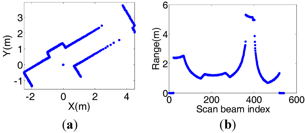
Figure 1. Corner measurements. (a) One of the corner scan scenes. (b) The corresponding range measurements.

From the scan scene, there are ten lines in total. However, when applying the breakpoint detection criterion and ignoring short segments containing less than N points, which tend to be scattered objects and are susceptible to noises and interferes, only three lines will be extracted, since corners cannot be identified. Here, N is the minimum number of points on the line and is set according to the distance from the scanned point to the sensor location.

Figure 2 demonstrates one of the scan scenes where three corners exist and are illustrated with red squares. After analyzing the pattern of corners, we realize that for M consecutive scan points, if a corner exists, the corresponding range measurement of the corner point is likely to be either the maximum or the minimum value among the M range measurements, as shown in Figure 2.

However, since LiDAR range measurements suffer from systematic and random noises, only detecting the maximum or minimum range measurement among M scan points can result in the detection of a spurious corner. To increase the robustness of the proposed line extraction method, the following criterion is added as a complementary to detect corners after the extremum r_m among M range measurements is detected:

$${\displaystyle \sum _{j=m-M/2}^{m+M/2}\left|r_m-r_j\right|}\ge r_{corner\_threshold}$$

(2)

where r_{corner_threshold} is the corner detection threshold. It is important to note for points on the same line feature, especially right beside the sensor, there will be points satisfying the second criterion. Therefore, the line feature will be detected as being more than one. However, this issue will be solved properly in the line merging process. Comparing our line extraction algorithm with the previous works, the corner problem is addressed, and iteration is not required.

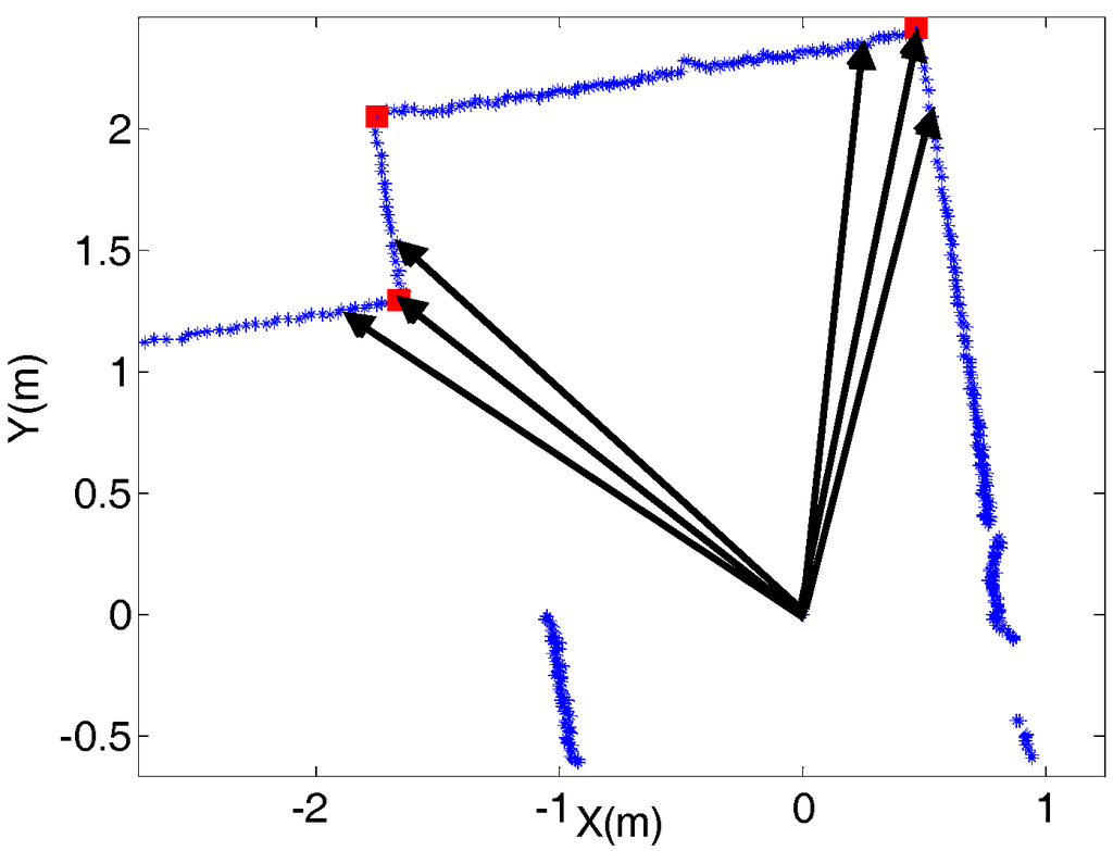
Figure 2. Corner detection.

Figure 2. Corner detection.

3.2. Line Parameters Calculation

After line segmentation, the weighted least squares method is used in our work to calculate the two line parameters in polar coordinate. The two parameters are the perpendicular distance from the origin of the vehicle body frame to the extracted line ρ and the angle between the x-axis of the body frame and the norm of the extracted line α, as shown in Figure 3.

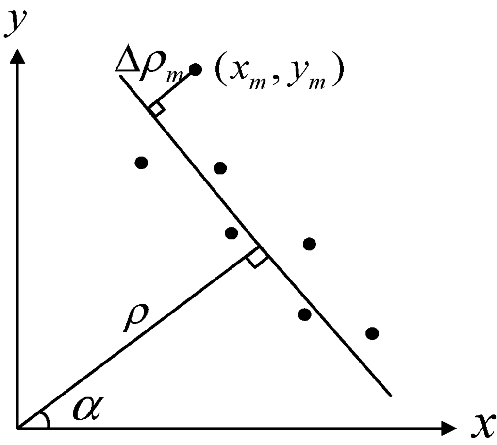
Figure 3. Line feature represented in the vehicle body frame.

Figure 3. Line feature represented in the vehicle body frame.

3.2.1. Scan Points’ Weight Calculation

Before applying weighted least squares to the line parameters estimation, the weight of each scan point is computed. Assuming that the diffuse component of the laser reflection is Lambertian, the following relation can be modeled [31]:

$$P_{return}\propto \frac{p\text{cos}\mathrm{\beta }}{r^2}$$

(3)

where P_return is the intensity of the returned laser pulse, p is the surface reflectance ranging from zero to one, β is the angle of incidence of the laser beam with the surface and r is the distance from the detected object to the sensor. As can be seen from this relation, the intensity is linked to the surface reflectivity, which will result in systematic error in range measurements [4]. Hence, the intensity will be used to weight the noise level in each LiDAR scanned point.

Regarding consecutive points on the same line segment, they share the same surface reflectance, and the difference between the corresponding range measurements is very small. The only significant difference is the incidence angle of the laser beam with the surface.

The reflected intensity of the m-th laser beam can be given as:

$$P_m\propto \frac{p\text{cos}({\text{θ}}_m-\mathrm{\alpha })}{r_m}$$

(4)

where θ_m is the bearing of the m-th laser beam. Assume that consecutive points on the same line segment have the same range measurements and differential intensities; we can get:

$$\mathrm{\Delta }{P}_{m,m+1}\propto \frac{p}{r_m}\left[\text{cos}({\text{θ}}_{m+1}-\mathrm{\alpha })-\text{cos}({\text{θ}}_m-\mathrm{\alpha })\right]$$

(5)

Apply the Taylor series to approximate the cosine function in the above equation, and only keep the first two terms; this can be rewritten as:

$$\mathrm{\Delta }{P}_{m,m+1}\propto \frac{p}{2r_m}\left(-\mathrm{\Delta }\text{θ}\right)\left(2{\text{θ}}_{m+1}-\mathrm{\Delta }\text{θ}-2\mathrm{\alpha }\right)$$

(6)

where Δθ is the bearing difference of two consecutive laser beams, also called the angle resolution. If we differentiate the intensity changes, the following relation can be derived:

$$\nabla \mathrm{\Delta }{P}_{m-1,m+1}\propto -\frac{p}{r_m}{\left(\mathrm{\Delta }\text{θ}\right)}^2$$

(7)

The angle resolution in our work is 0.5 degrees. Transformed to radians and squared, the numerator is at a magnitude of 10⁻⁶, which indicates that the double difference of the consecutive points’ intensity measurements is approximately zero. Therefore, for points on the same line segment, the double difference of their intensities should be very close to zero. Significant deviation from zero is mainly caused by errors and will be used as the weight for the scan points. The more significant the deviation is, the lower the weight is.

3.2.2. Line Parameters Estimation

After deriving the weight for each scan point, the line parameters ρ and α are estimated. Line parameters estimation is the problem of minimizing the sum of the squared normal distance from each point to the detected line [6]. The cost function is given as:

$$\text{min}{\displaystyle \sum w_m{\left(\text{ρ}-x_m\text{cos}\mathrm{\alpha }-y_m\text{sin}\mathrm{\alpha }\right)}^2}$$

(8)

Here, (x_m, y_m) are the coordinates of the m-th scan point in the Cartesian frame. The least-squares-based solution for the above cost function is given as follows [6]:

$$\mathrm{\alpha }=\frac{1}{2}\text{arctan}(\frac{-2S_{xy}}{S_{yy}-S_{xx}})$$

(9)

$$\text{ρ}=\overline{x}\text{cos}\mathrm{\alpha }+\overline{y}\text{sin}\mathrm{\alpha }$$

(10)

where $S_{xy}={\displaystyle \sum w_m(x_m-\overline{x})(y_m-\overline{y})}$, $S_{yy}={\displaystyle \sum w_m}{(y_m-\overline{y})}^2$, $S_{xx}={\displaystyle \sum w_m{(x_m-\overline{x})}^2}$, $\overline{x}=\frac{1}{{\displaystyle \sum w_m}}{\displaystyle \sum w_m{x}_m}$, $\overline{y}=\frac{1}{{\displaystyle \sum w_m}}{\displaystyle \sum w_m{y}_m}$.

3.2.3. Line Quality Calculation

To evaluate the line extraction error, we define a parameter, line quality. When the residual of the cost function displayed in Equation (8) is small, we assume that the line extraction error is small and that the quality of the line is good, and vice versa. Before giving the definition for the line quality parameter, we first define the perpendicular distance from the m-th scan point to the line as Δρ_m, as demonstrated in Figure 3. It can be depicted as:

$$\mathrm{\Delta }{\text{ρ}}_m=\text{ρ}-x_m\text{cos}\mathrm{\alpha }-y_m\text{sin}\mathrm{\alpha }$$

(11)

The quality of the k-th line feature q_k is thereafter defined as the covariance of the perpendicular distance deviation of all of the n points on the line, denoted as:

$$q_k=\text{cov}(\mathrm{\Delta }{\text{ρ}}_1,\dots ,\mathrm{\Delta }{\text{ρ}}_n)$$

(12)

When estimating pose change and the associated covariance in the following line feature matching process, a line feature with a big extraction error will be given less weight, and a line feature of good quality will have a big weight.

3.3. Line Merging

There are cases when a line feature in the real world is partly blocked or interrupted. To this end, more than one line representing the same line feature will be extracted. Merging these lines can gain more reliable line features and enable the line feature matching process to be more efficient. The line merging criterion is to compare the parameters of the detected line features, since the line parameters of the same line feature should be close. If the differences between the line parameters are small, the lines are merged, and new line parameters are recomputed.

3.4. Pose Change and Covariance Estimation

After line features are extracted and merged, the same line features occurring in the two consecutive scans are matched to derive the relative position and azimuth (pose) changes. The line feature matching is implemented by checking each line feature in the previous scan against the line features in the next scan. If the relative azimuth and perpendicular distance changes are close within a threshold, a matched line feature pair is declared. To illustrate how vehicle pose change is derived from line feature matching, Figure 4 shows the same line feature (shown in red) in the body frame at epoch i and i + 1. The relative position changes along both axes are defined as Δx and Δy while the azimuth change is defined as ΔA_i,i+1.

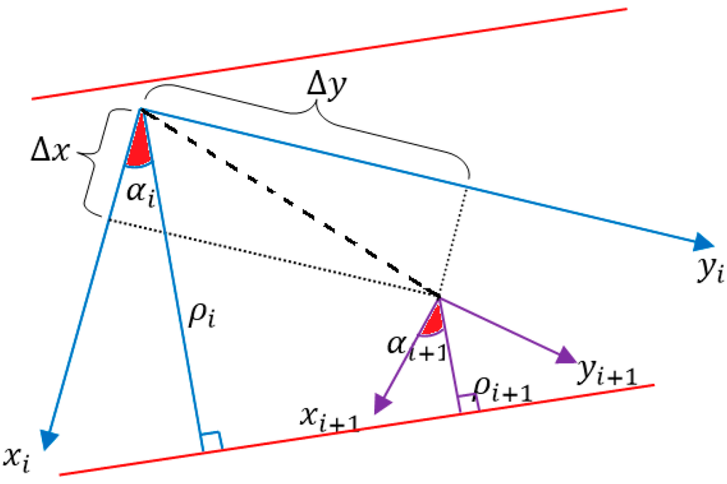
Figure 4. The vehicle pose change over two consecutive scans.

Figure 4. The vehicle pose change over two consecutive scans.

3.4.1. Position Change and Covariance Estimation

The relation between perpendicular distance change and relative position change is given as below:

$$\mathrm{\Delta }{\text{ρ}}_{i,i+1}={\text{ρ}}_i-{\text{ρ}}_{i+1}=\mathrm{\Delta }x\text{cos}{\mathrm{\alpha }}_i+\mathrm{\Delta }y\text{sin}{\mathrm{\alpha }}_i$$

(13)

Assume that k line features are extracted and matched for two consecutive scans; Equation (13) can be rewritten as:

$$\left[\begin{array}{c}\mathrm{\Delta }{\text{ρ}}_{i,i+1,1}\\ \begin{array}{c}\dots \\ \mathrm{\Delta }{\text{ρ}}_{i,i+1,k}\end{array}\end{array}\right]=H_{\text{ρ}}\left[\begin{array}{c}\mathrm{\Delta }x\\ \mathrm{\Delta }y\end{array}\right]=\left[\begin{array}{c}\begin{array}{cc}\text{cos}{\mathrm{\alpha }}_{i,1}& \text{sin}{\mathrm{\alpha }}_{i,1}\end{array}\\ \begin{array}{c}\begin{array}{cc}\dots & \dots \end{array}\\ \begin{array}{cc}\text{cos}{\mathrm{\alpha }}_{i,k}& \text{sin}{\mathrm{\alpha }}_{i,k}\end{array}\end{array}\end{array}\right]\left[\begin{array}{c}\mathrm{\Delta }x\\ \mathrm{\Delta }y\end{array}\right]$$

(14)

Here, Δρ_i,i+1,j is the perpendicular distance change of the j-th pair of the matched line feature between epoch i and i + 1. H_ρ is the design matrix with elements that are cosine and sine terms of α_i,j, while α_i,j is the angle parameter of the j-th pair of the matched line feature in epoch i, j = 1, …, k. Applying weighted least squares, the solution of the displacement vector can be given as:

$$\left[\begin{array}{c}\mathrm{\Delta }x\\ \mathrm{\Delta }y\end{array}\right]={(H_{\text{ρ}}^{T}W{H}_{\text{ρ}})}^{-1}{H}_{\text{ρ}}^{T}W\left[\begin{array}{c}\mathrm{\Delta }{\text{ρ}}_{i,i+1,1}\\ \begin{array}{c}\dots \\ \mathrm{\Delta }{\text{ρ}}_{i,i+1,k}\end{array}\end{array}\right]$$

(15)

where W is the diagonal matrix representing the weight of the observation vector, which is the perpendicular distance change vector. The j-th element (j = 1, …, k) of W is denoted as:

$$W_j=\frac{1}{q_{i,j}+q_{i+1,j}}$$

(16)

where q_i,j and q_i+1,j are derived from line quality calculation Equation (12). By defining in this way, the weight of the matched line feature pair is inversely proportional to the line extraction errors of the matched lines. The covariance matrix of the displacement vector can then be given as follows:

$$C_{\mathrm{\Delta }x,\mathrm{\Delta }y}={(H_{\text{ρ}}^{T}W{H}_{\text{ρ}})}^{-1}{\mathrm{\sigma }}_{\text{ρ}}^2$$

(17)

where ${\mathrm{\sigma }}_{\text{ρ}}^2$ is the perpendicular distance change error variance.

3.4.2. Azimuth Change and Covariance Estimation

The relation between line feature angle change and vehicle azimuth change is straightforward, which can be represented as:

$$\mathrm{\Delta }{A}_{i,i+1}={\mathrm{\alpha }}_{i+1}-{\mathrm{\alpha }}_i$$

(18)

Similarly, given k observations, the azimuth change $\mathrm{\Delta }{A}_{i,i+1}$ can be expressed as:

$$\left[\begin{array}{c}\mathrm{\Delta }{\mathrm{\alpha }}_{i,i+1,1}\\ \begin{array}{c}\dots \\ \mathrm{\Delta }{\mathrm{\alpha }}_{i,i+1,k}\end{array}\end{array}\right]=H_{\mathrm{\alpha }}\mathrm{\Delta }{A}_{i,i+1}={\left[\begin{array}{ccc}1& \dots & 1\end{array}\right]}^T\mathrm{\Delta }{A}_{i,i+1}$$

(19)

where Δα_i,i+1,j is the line feature angle change of the j-th pair of the matched line feature between epoch i and i + 1, j = 1, …, k. H_α is a vector with elements of one. Applying weighted least squares, the solution of the azimuth change can be given as:

$$\mathrm{\Delta }{A}_{i,i+1}={(H_{\mathrm{\alpha }}^{T}W{H}_{\mathrm{\alpha }})}^{-1}{H}_{\mathrm{\alpha }}^{T}W\left[\begin{array}{c}\mathrm{\Delta }{\mathrm{\alpha }}_{i,i+1,1}\\ \begin{array}{c}\dots \\ \mathrm{\Delta }{\mathrm{\alpha }}_{i,i+1,k}\end{array}\end{array}\right]$$

(20)

where W is the diagonal matrix representing the weight of each pair of matched line feature angle parameter changes between continuous scans. It is defined by Equation (16).

For the covariance of the azimuth change, this is given as:

$$C_{\mathrm{\Delta }A}={(H_{\mathrm{\alpha }}^{T}W{H}_{\mathrm{\alpha }})}^{-1}{\mathrm{\sigma }}_{\mathrm{\alpha }}^{\text{2}}$$

(21)

where ${\mathrm{\sigma }}_{\mathrm{\alpha }}^{\text{2}}$ is the line feature angle change error variance.

3.4.3. Singularity Issue

As pointed out by [8], the transformation from line extraction errors into position error is determined by the line geometry. More specifically, when only one line feature or only parallel line features are matched, the relative position change solutions of the weighted least squares will be singular, since the rank of the design matrix will be less than the number of the expected variables, which is two in this case. This is an issue occurring especially in long corridors. On the contrary, when at least two perpendicular lines are matched, the singularity issue will not exist, and the relative position change can be accurately estimated. Therefore, it is essential that the estimated position change covariance can reveal the influence of the line geometry. Besides, the limitation of LiDAR navigating in long corridors also makes the integration of LiDAR and INS of great significance. When the singularity issue occurs, the inverse of H_ρ^TWH_ρ in Equations (15) and (17) will be significantly large. Therefore, the estimated position change will be erroneous, and the associated covariance estimation will be large. In the fusion with the gyroscope and odometer through the filter, the erroneous updates will be reflected by the estimated observation covariance, and consequently, the filter will trust the prediction from the system model more than the LiDAR-derived measurements in this case. It is important to mention that the singularity issue does not exist in the azimuth change estimation.

4. The Integrated Solution and Filter Design

In this section, the integrated solution is described. The main motion model of the proposed system is an INS supported by odometer measurements. Inertial sensors can provide angular velocity and acceleration, while the odometer can provide linear velocity. They are independent of the operating environment, but suffer from error accumulation. On the other side, pose tracking using LiDAR line feature-based scan matching has long-term consistent accuracy, but it is susceptible to the environment’s structure. To achieve better performance than using any sensor unaided, the three sensors are integrated through an EKF. One innovation of our filter design is that only one vertical gyroscope is used without the accelerometer, given the assumption that land-based vehicles, especially UGVs, mostly move in horizontal planes [32,33]. The benefits are the lower cost and less complexity in mechanization. More importantly, velocity is derived from the odometer instead of the integration results of the accelerometer outputs; hence, the error in velocity is reduced. The block diagram of the multi-sensor integrated navigation system is demonstrated in Figure 5.

More specifically, a single-axis gyroscope vertically aligned with the vehicle body frame is used to detect the rotation rate of the body frame with respect to the inertial frame, from which the azimuth can be yielded. The odometer can output velocity along the direction where the vehicle moves forward. By integrating the single-axis gyroscope and odometer, the vehicle motion change from dead reckoning can be derived. Meanwhile, the pose change and covariance can be derived from LiDAR based on the proposed algorithm. Due to the nonlinearity of the system, the EKF is adopted to fuse the information from different sensors. Then, the gyroscope bias is accurately estimated, and the navigation solutions are corrected.

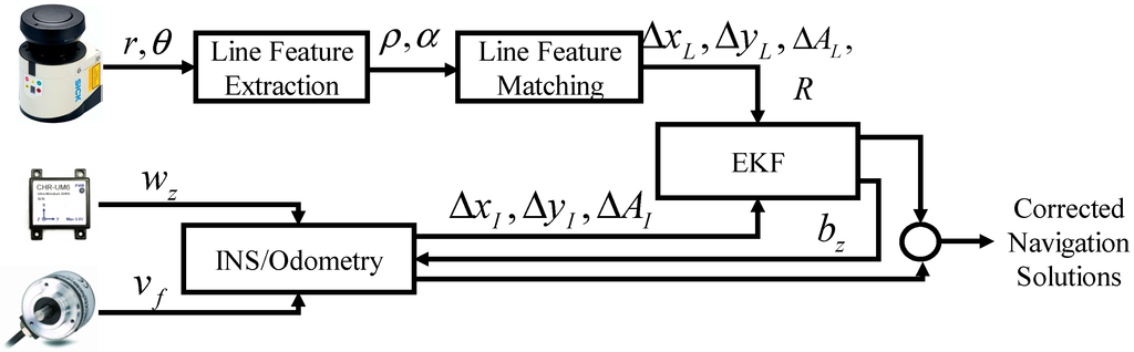
Figure 5. The block diagram of the multi-sensor integrated navigation system.

Figure 5. The block diagram of the multi-sensor integrated navigation system.

4.1. System Model

The error state vector for the filter design is defined as:

$$\text{δ}x={\left[\text{δ}\mathrm{\Delta }x \text{δ}\mathrm{\Delta }y \text{δ}{v}_f \text{δ}{v}_x\text{ δ}{v}_y \text{δ}\mathrm{\Delta }A \text{δ}{a}_{od} \text{δ}{b}_z\right]}^T$$

where the variables are defined as below: δΔx is the error in the relative displacement between scans along the x-axis in the vehicle body frame; δΔy is the error in the relative displacement between scans along the y-axis in the vehicle body frame; δv_f is the error in the forward speed derived from the odometer; δv_x is the error in the forward velocity projecting along the x-axis in the vehicle body frame; δv_y is the error in the forward velocity projecting along the y-axis in the vehicle body frame; δΔA is the error in the azimuth change between scans; δa_od is the error in acceleration derived from the odometer measurements; δb_z is the error in the gyroscope bias.

The system model is derived from INS/odometry mechanization. Specifically, the azimuth change between two scans can be calculated using gyroscope measurements. It is given as follows:

$$\mathrm{\Delta }{A}_I=-(w_z-b_z)T$$

(22)

where ΔA_I is the azimuth change obtained from INS, w_z is the gyroscope measurement, b_z is the gyroscope bias and T is the time interval between two scans. Based on the azimuth change, forward velocity can be projected to the vehicle body frame:

$$v_x=v_f\text{sin}(\mathrm{\Delta }{A}_I)$$

(23)

$$v_y=v_f\text{cos}(\mathrm{\Delta }{A}_I)$$

(24)

Therefore, the relative position change between two scans can be denoted as:

$$\mathrm{\Delta }{x}_I=v_{x}T$$

(25)

$$\mathrm{\Delta }{y}_I=v_{y}T$$

(26)

By applying Taylor expansion to the INS/odometry dynamic system given in Equations (22)–(26) and considering only the first order term, the linearized dynamic system error model is given as below [34,35]:

$$\text{δ}\mathrm{\Delta }\dot{x}=\text{δ}{v}_x$$

(27)

$$\text{δ}\mathrm{\Delta }\dot{y}=\text{δ}{v}_y$$

(28)

$$\text{δ}{\dot{v}}_f=\text{δ}{a}_{od}$$

(29)

$$\text{δ}{\dot{v}}_x=\text{sin}\left(\mathrm{\Delta }A\right)\text{δ}{a}_{od}+\text{cos}\left(\mathrm{\Delta }A\right)\left(w_z-b_z\right)\text{δ}{v}_f-v_f\text{cos}(\mathrm{\Delta }A)\text{δ}{b}_z+\left[a_{od}\text{cos}\left(\mathrm{\Delta }A\right)-v_f\text{sin}\left(\mathrm{\Delta }A\right)\left(w_z-b_z\right)\right]\text{δ}\mathrm{\Delta }A$$

(30)

$$\text{δ}{\dot{v}}_y=\text{cos}\left(\mathrm{\Delta }A\right)\text{δ}{a}_{od}-\text{sin}\left(\mathrm{\Delta }A\right)\left(w_z-b_z\right)\text{δ}{v}_f+v_f\text{sin}(\mathrm{\Delta }A)\text{δ}{b}_z-\left[a_{od}\text{sin}\left(\mathrm{\Delta }A\right)+v_f\text{cos}\left(\mathrm{\Delta }A\right)\left(w_z-b_z\right)\right]\text{δ}\mathrm{\Delta }A$$

(31)

$$\text{δ}\mathrm{\Delta }\dot{A}=-\text{δ}{b}_z$$

(32)

$$\text{δ}{\dot{a}}_{od}=-{\text{γ}}_{od}\text{δ}{a}_{od}+\sqrt{2{\text{γ}}_{od}{\text{σ}}_{od}^2}w$$

(33)

$$\text{δ}{\dot{b}}_z=-{\text{β}}_z\delta b_z+\sqrt{2{\text{β}}_z{\text{σ}}_z^2}w$$

(34)

Here, both random errors in acceleration derived from odometer and gyroscope measurements are modeled as first order Gauss–Markov processes. γ_od and β_z are the reciprocal of the correlation time constants of the random process, while σ_od and σ_z are the standard deviations associated with the odometer and gyroscope measurements, respectively.

4.2. Measurement Model

For the measurement model, the pose changes estimated from the line feature scan matching are used as filter observations, and the observation covariance matrix is also adaptively calculated by the proposed technique. The advantages of this filter design are two-fold: (1) the line geometry influence is taken into account when estimating the observation covariance; thus, it can precisely reflect the error level in the observations; (2) the tuning of the observation covariance matrix is avoided.

The difference of vehicle pose change between scans obtained from INS/odometry and LiDAR is taken as the observation vector in the measurement model. The observation vector is defined by z and can be given as:

$$z=\left[\begin{array}{c}\mathrm{\Delta }{x}_L-\mathrm{\Delta }{x}_I\\ \mathrm{\Delta }{y}_L-\mathrm{\Delta }{y}_I\\ \mathrm{\Delta }{A}_L-\mathrm{\Delta }{A}_I\end{array}\right]$$

(35)

The subscript L and I denote measurements from LiDAR and INS, respectively. Therefore, the design matrix for the measurement model can be represented as:

$$\text{H}=\left[\begin{array}{cc}\begin{array}{ccc}1& 0& 0\\ 0& 1& 0\\ 0& 0& 0\end{array}& \begin{array}{cc}\begin{array}{ccc}0& 0& 0\\ 0& 0& 0\\ 0& 0& 1\end{array}& \begin{array}{cc}0& 0\\ 0& 0\\ 0& 0\end{array}\end{array}\end{array}\right]$$

(36)

For the observation covariance matrix R, it is assumed to be a diagonal matrix without considering the correlation between relative displacement and azimuth change. It is given as:

$$R=diag(C_{\mathrm{\Delta }x,\mathrm{\Delta }y},C_{\mathrm{\Delta }A})$$

(37)

Here, C_Δx,Δy and C_ΔA are calculated using Equations (17) and (21), respectively.

After establishing the system model and measurement model, EKF equations are used to implement the prediction and correction. The prediction and correction are performed in the body frame and then transformed into the navigation frame to provide corrected navigation outputs.

5. Experiment Results and Analysis

To evaluate the proposed algorithm, real experiments have been performed in an indoor office building with a UGV called Husky A200 from Clearpath Robotics Inc. (Waterloo, Canada), shown in Figure 6. This UGV is wirelessly controlled, and the platform is equipped with a CHR-UM6 MEMS-grade inertial measurement unit (IMU) [36], a SICK laser scanner LMS111 (SICK, Waldkirch, Germany) [37] and a quadrature encoder. The specifications of the laser scanner are shown in Table 1.

The experiment is conducted on the second floor of the building, with the UGV moving in the corridor during the whole process. The spatial layout of the floor is an approximate 70 m by 40 m rectangle, shown in Figure 7.

As can be seen from the floor plan, the corridor length sometimes can exceed the maximum scanning range of the LiDAR, which is 20 m in our experiments. This may result in the singularity problem. From the earlier discussion, it can be seen that a poor geometric layout can cause the singularity issue, and the estimated covariance will be large. Meanwhile, due to the proper weighting scheme for the line feature in the covariance estimation process, a large line extraction error will not jeopardize the estimation accuracy of the relative position change and associated covariance. To address the influences of geometry layout and line quality on the relative position change and the covariance estimation, two cases are discussed. The LiDAR scans under these two situations are shown in Figure 8 and Figure 9 with extracted lines marked. The green square represents the beginning of the line, and the red diamond means the end of the line. In both figures, the graph on the left shows the previous scan, while the graph on the right is the scan ten epochs later. The ten-epoch interval is to guarantee distinguishable changes can accumulate and be estimated.

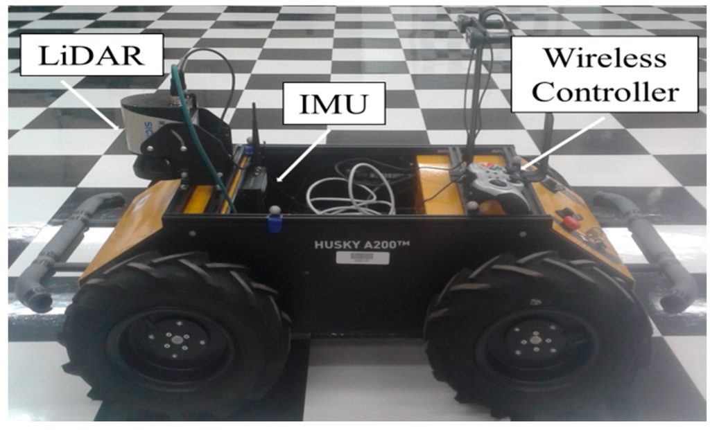
Figure 6. Husky A200.

Figure 6. Husky A200.

Table 1. SICK LMS111 specifications.

Parameter	Value
Statistical Error (mm)	±12
Angular Resolution (°)	0.5
Maximum Measurement Range (m)	20
Scanning Range (°)	270
Scanning Frequency (Hz)	50

Table 1. SICK LMS111 specifications.

Parameter	Value
Statistical Error (mm)	±12
Angular Resolution (°)	0.5
Maximum Measurement Range (m)	20
Scanning Range (°)	270
Scanning Frequency (Hz)	50

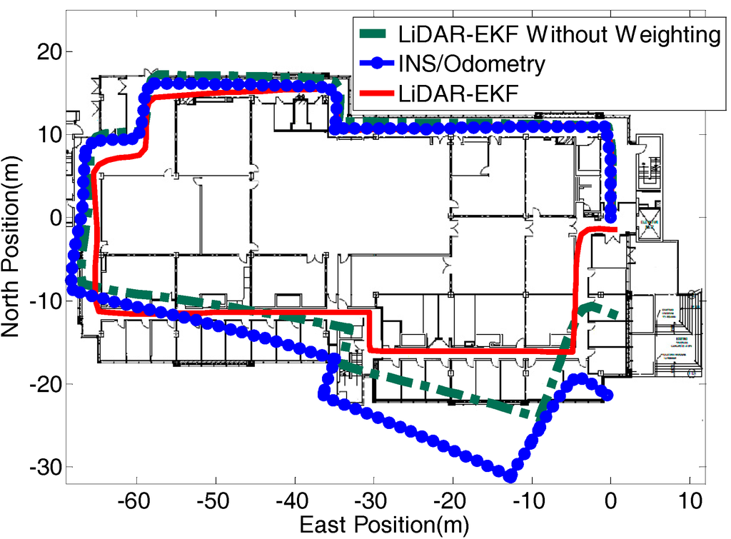
Figure 7. LiDAR-aided and INS/Odometry trajectories.

Figure 7. LiDAR-aided and INS/Odometry trajectories.

Figure 8 illustrates an example of when the UGV is located in the long corridor. In this case, only two parallel walls are detected, and two parallel line features will be matched between the two scans. The geometry layout will cause the singularity in the relative position change estimation. However, since the scan points on the extracted lines are well distributed, the line quality is good.

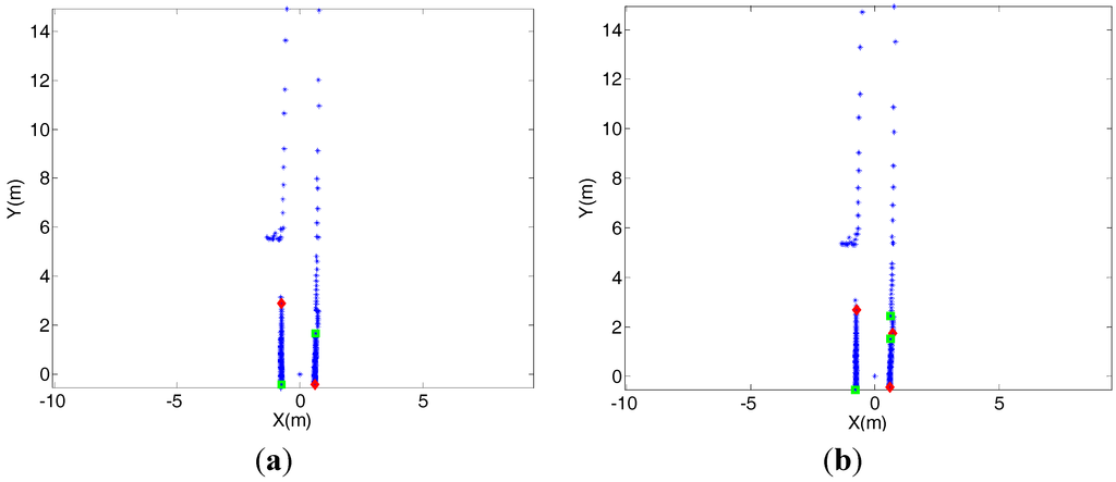
Figure 8. UGV moves in the long corridor. (a) The first scan. (b) The second scan.

Figure 8. UGV moves in the long corridor. (a) The first scan. (b) The second scan.

Figure 9 demonstrates another example when the UGV comes to a corner. Four lines are extracted in the first scan, while five lines are extracted in the second scan. In the line matching step, the first three lines in both scans are matched successfully, while the fourth line in the first scan is matched with the fifth line in the second scan. For the four pairs of matched lines, the line extraction errors of the first two pairs are small. The third pair’s line extraction error will increase, while the last pair’s line extraction error will be the most significant. As indicated by Equation (16), the bigger the line extraction error is, the lower the weight that will be given to the corresponding line pair in the line feature scan matching-based pose change and covariance estimation process. To this end, the mismatched fourth line pair will have the least weight in position change estimation.

Figure 9. The UGV arrives at a corner. (a) The first scan. (b) The second scan.

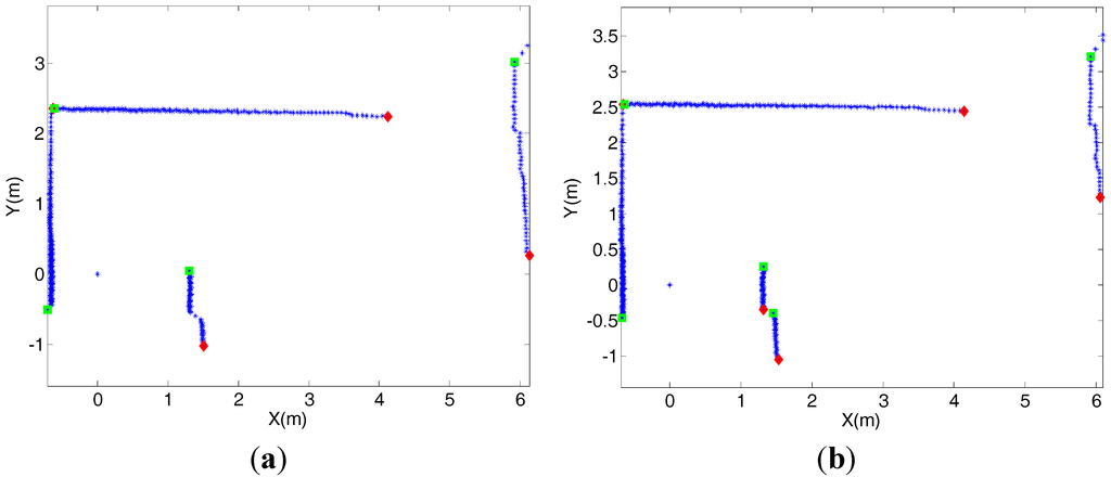
Figure 9. The UGV arrives at a corner. (a) The first scan. (b) The second scan.

The relative displacement and covariance estimation results for the above two examples are shown in Table 2. Under both situations, the UGV mainly moves along the vertical direction of the body frame. The maximum speed of the vehicle is 1 m/s while ten epoch time interval is 0.2 s. Therefore, the results of example 2 are reasonable while the results of example 1 are quite erroneous. This leads to the conclusion that the geometry layout of the extracted lines has significant impact on the estimation of the displacement. On the contrary, since the line feature is weighted by its quality in displacement estimation, line quality has minor effect on the results. However, the covariance of the displacement estimated from the proposed algorithm can reflect the error level in position change precisely. When the displacement is propagated to the filter, the observation can be evaluated according to its covariance and accurate error states estimation can be achieved.

Table 2. SICK LMS111 specifications.

Example	Δx (m)	Δy (m)	Cov (Δx)	Cov (Δy)
Example 1	0.3801	30.1185	0.0041	20.6805
Example 2	0.0602	0.2057	0.0001025	0.0001956

Table 2. SICK LMS111 specifications.

Example	Δx (m)	Δy (m)	Cov (Δx)	Cov (Δy)
Example 1	0.3801	30.1185	0.0041	20.6805
Example 2	0.0602	0.2057	0.0001025	0.0001956

Figure 10 shows a portion of the relative position change in the vehicle forward direction from LiDAR and INS along with the estimated covariance. From the figure, it can be clearly seen that when the LiDAR-derived position change is accurate, the estimated covariance is very small. On the contrary, when the LiDAR-derived position change is significantly jeopardized, the estimated covariance is fairly large. This demonstrates the consistency and the accuracy of the proposed covariance estimation method.

Figure 10. Relative position change in the vehicle forward direction from LiDAR and INS and the estimated covariance.

Figure 10. Relative position change in the vehicle forward direction from LiDAR and INS and the estimated covariance.

The trajectories obtained from the unaided INS/odometry dead reckoning system after initial gyroscope bias compensation and the LiDAR-aided integrated system are demonstrated on the floor plan. Besides, the filtered trajectory without weighting the scanned points in the line parameter estimation and without weighting the matched line pairs in the pose change and the associated covariance estimation are also shown in Figure 7. It is important to note that, even without the weighting scheme, the observation covariance still adaptively changes instead of being set to a fixed value. However, due to the inaccurate pose change and associated covariance estimation, the error in the navigation solutions accumulates gradually. Compared with the unaided and unweighted navigation solutions, the filtered navigation solutions show a significant improvement in accuracy. This means that with the corrections from the LiDAR and observation covariance matrix from the proposed algorithm, the gyroscope bias is precisely estimated (illustrated in Figure 11), which directly reflects the improved accuracy of the integrated solutions (the red curve in Figure 7).

Figure 11. Gyroscope bias estimation results.

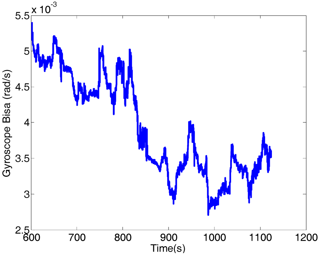
Figure 11. Gyroscope bias estimation results.

6. Conclusions

To overcome the challenge of indoor navigation and to address the limitations in the existing literature, this paper proposed a multi-sensor integrated navigation system that integrates a low-cost MEMS-grade inertial sensor gyroscope, odometer and ranging sensor LiDAR through an EKF. The paper introduced an adaptive covariance estimation method for LiDAR-estimated pose changes. The proposed EKF scheme benefited from the long-term accuracy of LiDAR and the self-contained dead reckoning INS to enhance the overall navigation solutions. The observations derived from LiDAR after line extraction and matching are relative position change and azimuth change. In the line extraction process, the LiDAR raw range and intensity measurements are used, and each scan point is weighted by the noise level in its range measurement. In the line matching step, the singularity issue and the line extraction error are addressed. Besides, the LiDAR observation covariance matrix is also estimated in the line matching step using weighted least squares. In the filter design, LiDAR observations and the observation covariance matrix are propagated to the measurement model. The real experiment results in an indoor building show that the observation covariance can precisely reflect the error level in the observations, and the error accumulation of the vehicle position is significantly reduced compared with the unaided solution.

References

- Gutmann, J.-S.; Schlegel, C. Amos: Comparison of scan matching approaches for self-localization in indoor environments. In Proceedings of the First Euromicro Workshop on Advanced Mobile Robot, Kaiserslautern, Germany, 9–11 October 1996; pp. 61–67.
- Hesch, J.A.; Mirzaei, F.M.; Mariottini, G.L.; Roumeliotis, S.I. A laser-aided inertial naviagtion system (L-INS) for human localization in unknown indoor environments. In Proceedings of the 2010 IEEE International Conference on Robotics and Automation (ICRA), Anchorage, AK, USA, 3–7 May 2010.
- Kohlbrecher, S.; Von Stryk, O.; Meyer, J.; Klingauf, U. A flexible and scalable slam system with full 3D motion estimation. In Proceedings of the 2011 IEEE International Symposium on Safety, Security, and Rescue Robotics (SSRR), 1–5 November 2011; pp. 155–160.
- Boehler, W.; Bordas Vicent, M.; Marbs, A. Investigating laser scanner accuracy. Int. Arch. Photogramm. Remote Sens. Spat. Inf. Sci. 2003, 34, 696–701. [Google Scholar]
- Martínez, J.L.; González, J.; Morales, J.; Mandow, A.; García-Cerezo, A.J. Mobile robot motion estimation by 2D scan matching with genetic and iterative closest point algorithms. J. Field Robot. 2006, 23, 21–34. [Google Scholar] [CrossRef]
- Garulli, A.; Giannitrapani, A.; Rossi, A.; Vicino, A. Mobile robot SLAM for line-based environment representation. In Proceedings of the 44th IEEE Conference on Decision and Control,2005 and 2005 European Control Conference (CDC-ECC'05), Seville, Spain, 12–15 December 2005; pp. 2041–2046.
- Arras, K.O.; Siegwart, R.Y. Feature Extraction and Scene Interpretation for Map-Based Navigation and Map Building; Intelligent Systems & Advanced Manufacturing, International Society for Optics and Photonics: Pittsburgh, PA, USA, 1998; pp. 42–53. [Google Scholar]
- Soloviev, A.; Bates, D.; van Graas, F. Tight coupling of laser scanner and inertial measurements for a fully autonomous relative navigation solution. Navigation 2007, 54, 189–205. [Google Scholar] [CrossRef]
- Pfister, S.T.; Roumeliotis, S.I.; Burdick, J.W. Weighted line fitting algorithms for mobile robot map building and efficient data representation. In Proceedings of the IEEE International Conference on Robotics and Automation (2003ICRA'03), 14–19 September 2003; pp. 1304–1311.
- Lingemann, K.; Nüchter, A.; Hertzberg, J.; Surmann, H. High-speed laser localization for mobile robots. Robot. Auton. Syst. 2005, 51, 275–296. [Google Scholar] [CrossRef]
- Aghamohammadi, A.A.; Taghirad, H.D.; Tamjidi, A.H.; Mihankhah, E. Feature-based range scan matching for accurate and high speed mobile robot localization. In Proceedings of the 3rd European Conference on Mobile Robots, Freiburg, Germany, 19–21 September 2007.
- Kammel, S.; Pitzer, B. Lidar-based lane marker detection and mapping. In Proceedings of the 2008 IEEE Intelligent Vehicles Symposium, Eindhoven, The Netherlands, 4–6 June 2008; pp. 1137–1142.
- Núñez, P.; Vazquez-Martin, R.; Bandera, A.; Sandoval, F. Fast laser scan matching approach based on adaptive curvature estimation for mobile robots. Robotica 2009, 27, 469–479. [Google Scholar] [CrossRef]
- Shen, S.; Michael, N.; Kumar, V. Autonomous multi-floor indoor navigation with a computationally constrained MAV. In Proceedings of the 2011 IEEE International Conference on Robotics and automation (ICRA), Shanghai, China, 9–13 May 2011; pp. 20–25.
- Segal, A.; Haehnel, D.; Thrun, S. Generalized-ICP. In Proceedings of the Robotics: Science and Systems 2009 Conference, University of Washington, Seattle, WA, USA, 28 June–1 July 2009.
- Censi, A. An ICP variant using a point-to-line metric. In Proceedings of the 2008 IEEE International Conference on Robotics and Automation (ICRA 2008), Pasadena, CA, USA, 19–23 May 2008; pp. 19–25.
- Weiß, G.; Puttkamer, E. A map based on laserscans without geometric interpretation. Intell. Auton. Syst. 1995, 4, 403–407. [Google Scholar]
- Censi, A.; Iocchi, L.; Grisetti, G. Scan matching in the Hough domain. In Proceedings of the 2005 IEEE International Conference on Robotics and Automation (ICRA 2005), Barcelona, Spain, 18–22 April 2005; pp. 2739–2744.
- Burguera, A.; González, Y.; Oliver, G. On the use of likelihood fields to perform sonar scan matching localization. Auton. Robot. 2009, 26, 203–222. [Google Scholar] [CrossRef]
- Olson, E.B. Real-time correlative scan matching. In Proceedings of the IEEE International Conference on Robotics and Automation (ICRA'09), Kobe, Japan, 12–17 May 2009; pp. 4387–4393.
- Diosi, A.; Kleeman, L. Laser scan matching in polar coordinates with application to SLAM. In Proceedings of the 2005 IEEE/RSJ International Conference on Intelligent Robots and Systems (IROS 2005), Edmonton, AB, Canada, 2–6 August 2005; pp. 3317–3322.
- Núñez, P.; Vázquez-Martín, R.; Del Toro, J.; Bandera, A.; Sandoval, F. Natural landmark extraction for mobile robot navigation based on an adaptive curvature estimation. Robot. Auton. Syst. 2008, 56, 247–264. [Google Scholar] [CrossRef]
- Borges, G.A.; Aldon, M.-J. Line extraction in 2D range images for mobile robotics. J. Intell. Robot. Syst. 2004, 40, 267–297. [Google Scholar] [CrossRef]
- Premebida, C.; Nunes, U. Segmentation and geometric primitives extraction from 2D laser range data for mobile robot applications. Robotica 2005, 2005, 17–25. [Google Scholar]
- Xia, Y.; Chun-Xia, Z.; Min, T.Z. Lidar scan-matching for mobile robot localization. Inf. Technol. J. 2010, 9, 27–33. [Google Scholar] [CrossRef]
- Ji, J.; Chen, G.; Sun, L. A novel hough transform method for line detection by enhancing accumulator array. Pattern Recognit. Lett. 2011, 32, 1503–1510. [Google Scholar] [CrossRef]
- Fernandes, L.A.; Oliveira, M.M. Real-time line detection through an improved hough transform voting scheme. Pattern Recognit. 2008, 41, 299–314. [Google Scholar] [CrossRef]
- Nguyen, V.; Martinelli, A.; Tomatis, N.; Siegwart, R. A comparison of line extraction algorithms using 2D laser rangefinder for indoor mobile robotics. In Proceedings of the 2005 IEEE/RSJ International Conference on Intelligent Robots and Systems (IROS 2005), Edmonton, AB, Canada, 2–6 August 2005; pp. 1929–1934.
- Diosi, A.; Kleeman, L. Uncertainty of line segments extracted from static SICK PLS laser scans, SICK PLS laser. In Proceedings of the Australiasian Conference on Robotics and Automation, Brisbane, Australia, 1–3 December 2003.
- Soloviev, A. Tight coupling of GPS and INS for urban navigation. Aerosp. Electron. Syst. IEEE Trans. 2010, 46, 1731–1746. [Google Scholar] [CrossRef]
- Hancock, J.; Hebert, M.; Thorpe, C. Laser intensity-based obstacle detection. In Proceedings of the 1998 IEEE/RSJ International Conference on Intelligent Robots and Systems, Victoria, BC, USA, 13–17 October 1998; pp. 1541–1546.
- Iqbal, U.; Okou, A.F.; Noureldin, A. An integrated reduced inertial sensor system—RISS/GPS for land vehicle. In Proceedings of the Position, Location and Navigation Symposium, 2008 IEEE/ION, Monterey, CA, USA, 5–8 May 2008; pp. 1014–1021.
- Iqbal, U.; Karamat, T.B.; Okou, A.F.; Noureldin, A. Experimental results on an integrated GPS and multisensor system for land vehicle positioning. Int. J. Navig. Obs. 2009, 2009, 765010. [Google Scholar]
- Liu, S.; Atia, M.M.; Karamat, T.; Givigi, S.; Noureldin, A. A dual-rate multi-filter algorithm for LiDAR-aided indoor navigation systems. In Proceedings of the Position, Location and Navigation Symposium-PLANS 2014, 2014 IEEE/ION, Monterey, CA, USA, 5–8 May 2014; pp. 1014–1019.
- Liu, S.; Atia, M.M.; Karamat, T.B.; Noureldin, A. A LiDAR-aided indoor navigation system for UGVs. J. Navig. 2014. [Google Scholar] [CrossRef]
- CHRobotics. UM6 ultra-miniature orientation sensor datasheet. Available online: http://www.chrobotics.com/docs/UM6_datasheet.pdf (accessed on 21 January 2015).
- SICK. Operating Instructions: LMS100/111/120 Laser Measurement Systems; SICK AG: Waldkirch, Germany, 2008. [Google Scholar]
© 2015 by the authors; licensee MDPI, Basel, Switzerland. This article is an open access article distributed under the terms and conditions of the Creative Commons Attribution license (http://creativecommons.org/licenses/by/4.0/).