Automatic Cloud and Shadow Detection in Optical Satellite Imagery Without Using Thermal Bands—Application to Suomi NPP VIIRS Images over Fennoscandia

Abstract

In land monitoring applications, clouds and shadows are considered noise that should be removed as automatically and quickly as possible, before further analysis. This paper presents a method to detect clouds and shadows in Suomi NPP satellite’s VIIRS (Visible Infrared Imaging Radiometer Suite) satellite images. The proposed cloud and shadow detection method has two distinct features when compared to many other methods. First, the method does not use the thermal bands and can thus be applied to other sensors which do not contain thermal channels, such as Sentinel-2 data. Secondly, the method uses the ratio between blue and green reflectance to detect shadows. Seven hundred and forty-seven VIIRS images over Fennoscandia from August 2014 to April 2016 were processed to train and develop the method. Twenty four points from every tenth of the images were used in accuracy assessment. These 1752 points were interpreted visually to cloud, cloud shadow and clear classes, then compared to the output of the cloud and shadow detection. The comparison on VIIRS images showed 94.2% correct detection rates and 11.1% false alarms for clouds, and respectively 36.1% and 82.7% for shadows. The results on cloud detection were similar to state-of-the-art methods. Shadows showed correctly on the northern edge of the clouds, but many shadows were wrongly assigned to other classes in some cases (e.g., to water class on lake and forest boundary, or with shadows over cloud). This may be due to the low spatial resolution of VIIRS images, where shadows are only a few pixels wide and contain lots of mixed pixels.

1. Introduction

Cloud and shadow detection in satellite images is a crucial step before analysis. Clouds and shadows disturb the modelling of land cover parameters from the reflectance values. With the new, frequently imaging satellites like Suomi NPP (National Polar-orbiting Partnership) and its potential to near real-time (NRT) operational applications, the detection method has to be robust and automated to allow for fast analysis without extra delays.

The Suomi NPP satellite was launched in October 2011 by NASA (National Aeronautics and Space Administration) to monitor and predict climate change and weather conditions over land, sea and atmosphere. Its optical VIIRS (Visible Infrared Imaging Radiometer Suite) instrument provides for instance critical data for environmental assessments, forecasts and warnings [1]. In this study the main motivation was to provide cloud free Suomi NPP VIIRS imagery for daily snow mapping of the Fennoscandia area.

The VIIRS cloud mask (VCM) algorithm was developed and tested in the Calibration-Validation (CalVal) program of the Joint Polar Satellite Systems [1,2]. The VCM algorithm uses both moderate resolution ’M’ bands (750 m at nadir) and the imagery resolution ’I’ bands (375 m at nadir) in pixel-level decisions on the presence of clouds [3]. The cloud tests used for each pixel are a function of the surface type: water, land, desert, coast, snow or ice, so these surface types have to be known beforehand in order to apply the VCM algorithm. The cloud tests differ also between daytime and night-time (solar zenith angle ≥85${}^{\circ }$) images. The cloud tests provide an overall probability of clouds, based on whether the pixel is finally classified as confidently cloudy, probably cloudy, probably clear or confidently clear. The method is clear sky conservative so that, also in the case of low probability of cloud, the pixel is not assigned as clear sky. The higher resolution ’I’ bands are used only after these initial assignments, and only to ocean-coast pixels to check and change from confidently clear to more cloudy classes.

Hutchinson et al. [3] compared the VCM mask to a manually generated cloud mask over Golden Granules and to CALIOP-VIIRS match-ups. The Golden Granules are binary cloud masks over challenging VIIRS instances assessed by several experts. CALIOP is a Cloud-Aerosol Lidar with Orthogonal Polarisation on board CALIPSO satellite (Cloud-Aerosol Lidar and Infrared Pathfinder Satellite Observation). VIIRS and CALIOP are in alignment for about 1–2 orbits every 3–4 days. However, the two sensors are within 20 min of each other, so the cloud situation has time to change. The important result was that the performance was consistent with both sources of reference data. Both manual and CALIOP-based cloud references showed almost as high a probability of correct classification to the clouds of VCM, each of them being a minimum of 93.9% on ocean, land, and desert backgrounds [3]. The percentage of missing and false alarms also fulfilled the performance goals for Validation Phase-2 maturity level of 1–8%.

Piper and Bahr [4] presented a rapid cloud-masking algorithm that used the ’I’ bands of the VIIRS imageös. It identified cloud pixels using reflectance values in 0.64 $\mathsf{\mu }$m, 0.865 $\mathsf{\mu }$m and 1.61 $\mathsf{\mu }$m, and temperature value in 11.45 $\mathsf{\mu }$m. Cloud pixels on snow covered areas were identified by first classifying the snow areas with the NDSI (Normalized Difference Snow Index [5,6]) and then identifying cloud pixels by the reflectance in 0.865 $\mathsf{\mu }$m. The results from this VIBCM (VIIRS I-Band Cloud Mask) algorithm were compared to the results from the VCM algorithm. The advantage of the VIBCM algorithm is that it can quickly compute the cloud mask at 375 m resolution. However, it was not as accurate as VCM. The hit rate of cloud pixels (cloud in both VCM and VIBCM cloud mask) was 72.0% in Hawaii area, 77.9% in Eastern United States area, and 94.5% in Northern Europe area. The corresponding false alarms rates (cloud in VIBCM cloud mask but not in VCM cloud mask) were 3.7%, 8.4% and 42.1%, respectively. Piper and Bahr pointed out three main issues with the method. The first was a likely temperature dependency. As the temperature values decrease from Hawaii to Northern Europe, the number of missing cloud pixels decreased but the number of false alarms increased. The other issue is that the accuracy assessment is done by comparison to the results of another cloud masking method, here VCM, which has its own accuracy issues. The third issue was that while one scene in the study had snow, the VIBCM failed to identify it. Piper and Bahr [4] concluded that additional work is needed to differentiate between snow and cold clouds with a range of VIIRS images that contain snow, cold surface temperatures and cold clouds. Shadow detection was not assessed in [4].

Cloud masking methods have been developed for MODIS (Moderate Resolution Imaging Spectro-radiometer) satellite images, which is the closest sensor to Suomi NPP VIIRS imagery for spatial resolution and spectral bands. Luo et al. [7] presented a method to classify cloud, shadow, snow and ice, water bodies, vegetated lands and non-vegetated lands from the MODIS 250-m imagery. The algorithm uses seven MODIS bands between 0.459 $\mathsf{\mu }$m and 2.155 $\mathsf{\mu }$m in 250 m resolution with a number of thresholds for reflectance values, differences and ratios. Shadows are mapped by the projection of clouds to the ground, using the sun angle and estimated elevation range from 0.5 km to 12 km. Shadow areas are confirmed with the ratios between 1.64 $\mathsf{\mu }$m and 0.47 $\mathsf{\mu }$m bands, and 0.86 $\mathsf{\mu }$m and 0.47 $\mathsf{\mu }$m bands. The accuracy assessment of the results was based on the visual comparison to MODIS standard cloud and shadow masks. The comparison showed more detailed and more comprehensive cloud and shadow masks. Luo et al. [7] concluded that more quantitative analyses are required to understand its performance over a range of input scenes in various seasons.

The SWIR (Short-Wave Infrared) band at 1.38 $\mathsf{\mu }$m (cirrus band), common to both in MODIS and VIIRS images, is located in a very strong water vapour absorption area and shows only the upper layers of the atmosphere. This has been used successfully to detect upper atmosphere clouds from MODIS imagery [8,9] and works well with thin cirrus clouds that are difficult to detect otherwise [10]. Zhu et al. [11] concluded that the cirrus band is more helpful than thermal band in cloud detection.

Snow and clouds have similar reflectance in the visible and near infrared (NIR) bands, but the reflectance of snow at 1.6 $\mathsf{\mu }$m is lower than that of clouds [12]. Both Piper and Bahr [4] and Dozier [12] mentioned the utilization of this band in the NDSI (Normalized Difference Snow Index) for snow detection, with the exception that Dozier proposed the utilization of green band and Piper and Bahr the utilization of the red band to normalize the difference index.

Metsämäki et al. [13] described a cloud screening method designed to be used for low-resolution satellite imagery, like Terra/MODIS, ERS-2/ATRS-2 (European Remote Sensing, Along Track Scanning Radiometer), Envisat/AATSR (Advanced Along Track Scanning Radiometer), Suomi NPP VIIRS, and future Sentinel-3 SLSTR (Sea and Land Surface Temperature Radiometer) imagery. The method uses the wavelength bands of 0.55 $\mathsf{\mu }$m, 1.6 $\mathsf{\mu }$m, 3.7 $\mathsf{\mu }$m, 11 $\mathsf{\mu }$m and 12 $\mathsf{\mu }$m, which are common to these sensors. The method is based on several empirically determined decision rules from selected training areas representing clouds, snow-covered terrain, partially snow-covered terrain and snow-free terrain. The method is used in the generation of GlobSnow data [13].

FMask is the state-of-the-art method for cloud, shadow and snow detection from Landsat 8 images. It uses the temperature bands to detect clouds at different heights [11,14]. The height of the cloud is then used also in shadow detection where the cloud is first projected to the ground before further analysis and detection of shadow pixels. The new Sentinel 2 optical imagery has all the same spectral bands as the VIIRS instrument. Zhu et al. [11] note that it is challenging to design a good cloud detection algorithm because Sentinel-2 does not have the thermal bands and most of the cloud detection algorithms are heavily dependent on the thermal band, as cloud pixels are much colder than clear-sky pixels.

Also multitemporal methods have been developed for cloud and shadow detection (Hagolle et al. [15] and Zhu et al. [16]). Multi-temporal cloud detection is usually more robust than single-date approaches. Multi-temporal approaches are well suited to time series analysis applications, however they increase significantly data volumes and computational costs for applications like single-date classifications over wide areas. Also, land cover changes bring new challenges to multi-temporal approaches. Single data approaches are easier to implement for NRT applications.

In this paper, we propose an automatic cloud and shadow detection method for optical satellite images (e.g., Suomi NPP VIIRS or Sentinel-2). In this paper, neither thermal bands nor multi-temporal analysis is used. Thermal bands are highly sensitive to atmospheric temperature variance during different seasons and consequently need time and space-specific thresholds [11]. One major advantage of not including the thermal bands in the algorithm is that the method is then also applicable to Sentinel-2 images that do not have these bands. For shadow detection, we present a novel method using the ratio between blue and green reflectances, that does not rely on cloud projection. The method is tested with VIIRS data in the boreal region with an abundance of dense forest intermingled with water areas, and snow and ice areas during several winter months. The test imagery covers Finland, large parts of Sweden and Norway, with snow covered mountains, and small parts of other neighbouring countries like Russia and the Baltic countries.

2. Suomi NPP VIIRS Imagery

Suomi NPP VIIRS images are acquired daily, with 5 high resolution bands (I-bands) at 375 m and 16 moderate resolution bands (M-bands) at 750 m. Because the M-bands include more spectral information for cloud detection and contain the spectral bands of Sentinel-2, M-bands were selected as the basis for cloud detection.

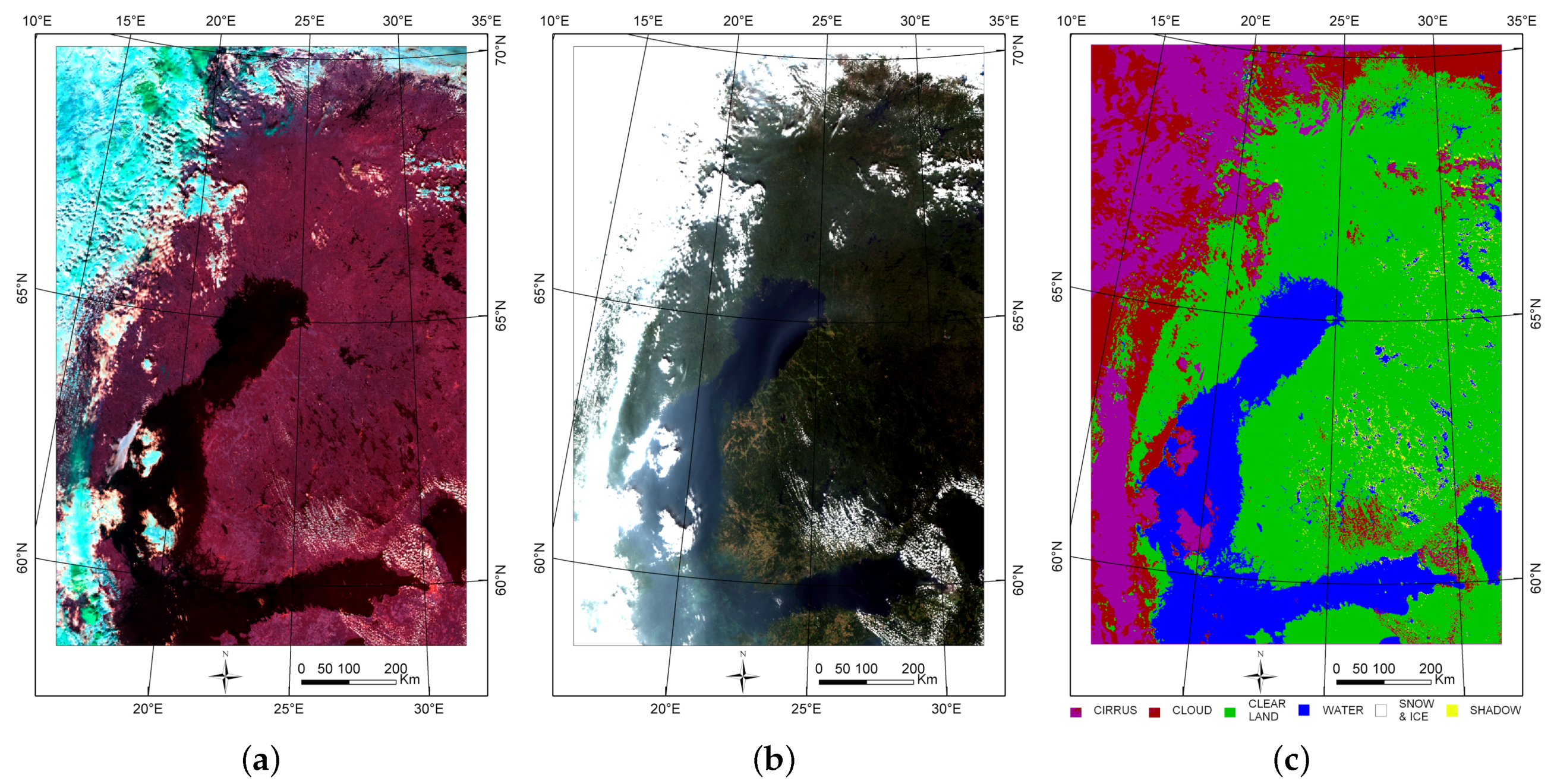
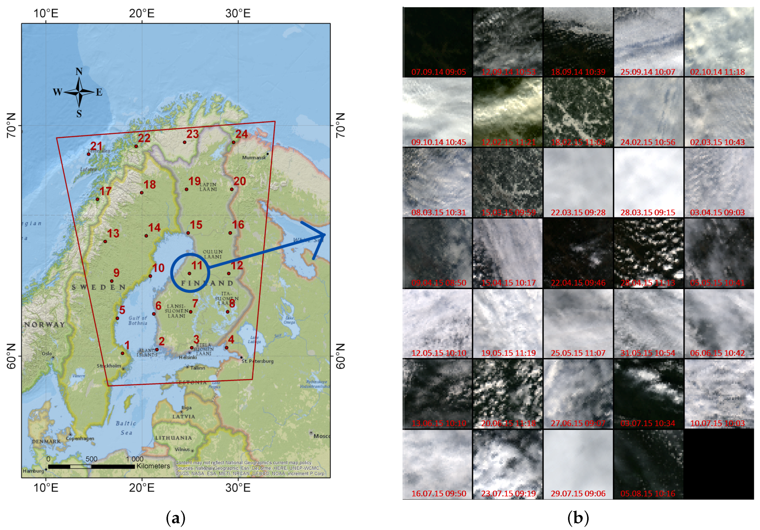
A total of 747 VIIRS images were acquired for the method development. The images were from boreal zone and cover Finland in total, as well as parts of Scandinavia and Russia—Figure 1a.

Seven hundred and forty-four VIIRS images (from 2 September 2014 to 25 April 2016) were loaded from the receiving station of the Finnish Meteorological Institute in Sodankylä, Finland, and to obtain some less cloudy summer images, three more images (4–6 August 2014) were downloaded from the CLASS (Comprehensive Large Array Stewardship System) archive of NOAA (National Oceanic and Atmospheric Administration). VIIRS images were georeferenced in Sodankylä, and only the relatively small rectified VIIRS images were downloaded to local computers. The images were resampled to 1 × 1 km${}^2$ pixel size in UTM zone 35/WGS84, Northern hemisphere, with nearest neighbour interpolation.

The atmospheric correction (conversion to surface reflectance or BOA reflectance—Bottom Of Atmosphere) of Suomi NPP/VIIRS data was implemented in the VTT in-house smac_viirs tool, which uses the SMAC algorithm (Simplified Model for Atmospheric Correction) by Rahman and Dedieu [17]. The following atmospheric values were used in the correction: Aerosol Optical Depth $AOD=0.01$, water vapour = 3.0 g/cm${}^2$, ozone = 0.3 atm/cm${}^2$ and pressure P = 1013 hpa. The low value of AOD was used in order to preserve the effect of clouds and haze in the reflectance values. At the time of processing (3 June 2015) there were no SMAC coefficient files for the bands of the VIIRS instrument. Coefficient files of the closest bands of other satellite sensors were used for VIIRS bands (see

Table 1. Bands of replacement sensors used for Suomi NPP/VIIRS bands in SMAC program.

VIIRS Band	Replacement Sensor	Band Index in Replacement Sensor
M1	Modis	8
M2	Modis	9
M3	Modis	10
M4	Landsat-8	3
M5	MISR	3
M6	Modis	15
M7	Modis	2
M8	Modis	5
M9	Modis	26
M10	Landsat-8	6
M11	Aster	7
I1	NOAA-18	1
I2	Modis	2
I3	Landsat-8	6

).

3. Methods

3.1. Cloud and Shadow Detection Algorithm

The starting point for the method was a cloud and shadow detection algorithm developed at VTT [18] for SPOT and Landsat images. This method was further developed to VIIRS images by adding new available bands and new rules to separate between cloud, shadow and other classes. This was done iteratively by executing the cloud and shadow detection algorithm, analysing the results and adding new land cover-specific rules to decrease missing and false detections. The spectral profiles of clouds, shadows and other land cover classes were compared visually to generate the new rules.

Table 2. VIIRS bands and their role in cloud and shadow detection and removal/separation of false cloud and shadow detections.

VIIRS Band	Name	Wavelength ($\mathsf{\mu }$m)	Applications
M2	Blue	0.445	Clouds, shadows, bare agricultural areas
M4	Green	0.555	Clouds, shadows, water, snow, bare agricultural areas
M5	Red	0.672	Clouds, clear land, bare agricultural areas
M7	NIR08	0.865	Shadows, water, bare agricultural areas
M9	NIR13	1.39	Cirrus clouds, shadows
M10	NIR16	1.61	Snow and ice
M11	NIR22	2.25	Clear land, shadows

shows the wavelength bands of VIIRS images that are used in the cloud and shadow detection algorithm.

Figure 2 shows the overall logic to classify VIIRS reflectance into the target classes. The output mask is initialised to land class (clear pixel). First, the method assigned cloud, shadow, snow, water and cirrus to pixels that satisfy rules 1, 7, 5, 9 and 4, respectively. These first rules were such that all cloud and shadow pixels were labelled, even at the cost of false alarms. Then part of the cloud pixels (bright urban and built areas, sand, bare agricultural fields) were assigned to clear land if any of the rules 2, 3 or 6 are true. Further, part of the clear land (dark dense forest) was reassigned to shadow with rule 8, and finally part of the shadows was reassigned to water with rule 10.

The rules are given in the following subsections, using logical connective operators ∧ (“AND”), ∨ (“OR”), → (“IMPLIES”, i.e., class assignment).

3.1.1. Cloud Masking Rules

Cloud class was initially assigned to the pixel if red, green and blue reflectances were all above a given threshold ($MIN\_REF=8.0\%$):

$$\begin{array}{c}(Blue>MIN\_REF)\wedge (Green>MIN\_REF)\wedge (Red>MIN\_REF)\to CLOUD\hfill \end{array}$$

(1)

Clear land was separated from cloud class with the following rules:

$$\begin{array}{c}\left(\frac{Red}{MIN\_REF}<1.5\right)\wedge \left(\frac{Red}{NIR22}>1.3\right)\to CLEAR\hfill \end{array}$$

(2)

$$\begin{array}{c}(NIR16<10\%)\wedge (NIR22<10\%)\to CLEAR\hfill \end{array}$$

(3)

Cirrus cloud was mapped from the cirrus band by threshold ($MIN\_CIRRUS=0.8\%$):

$$\begin{array}{c}(NIR13>MIN\_CIRRUS)\to CIRRUS\hfill \end{array}$$

(4)

Snow was separated from cloud class with the Normalised Difference Snow Index [5,6] ($MIN\_SNOWINDEX=0.7\%$):

$$\begin{array}{cc}\hfill & (NDSI>MIN\_SNOWINDEX)\wedge (NIR13<100\%)\to SNOW\hfill \\ \hfill \mathrm{with}& NDSI=\frac{(Green---NIR16)}{(Green+NIR16)}\hfill \end{array}$$

(5)

Agricultural areas were removed from the cloud layer with the reflectance in 0.865 $\mathsf{\mu }$m. If it was at least twice higher than in visible bands, the pixel was changed from cloud to clear area:

$$\begin{array}{c}\left(Max\right(2·Blue,2·Green,2·Red,NIR08)=NIR08)\to CLEAR\hfill \end{array}$$

(6)

3.1.2. Shadow Masking Rules

Cloud shadow was mapped with following rules ($MAX\_NIR=8.0\%$):

$$\begin{array}{cc}\hfill & \left((Red<4.0\%)\wedge (Red>NIR22)\right)\wedge \hfill \\ \hfill & [\left((NIR08>Red)\wedge (NIR08>NIR22)\right)\hfill \\ \hfill \vee & \hfill \\ \hfill & \left((Red<MIN\_REF)\wedge (Green<MIN\_REF)\wedge (Blue<MIN\_REF)\wedge (NIR08>5.0\%)\right)\hfill \\ \hfill \vee & \hfill \\ \hfill & (NIR08<MAX\_NIR)]\to SHADOW\hfill \end{array}$$

(7)

Cloud shadow was extracted from dark dense vegetation areas and water boundary areas with the following rule ($MIN\_SHADOW=1.2\%$):

$$\begin{array}{cc}(Blue/Green>MIN\_SHADOW)\to SHADOW\hfill & \hfill \end{array}$$

(8)

3.1.3. Water Masking Rules

Water was mapped with the following rules:

$$\begin{array}{c}(NIR08<12\%)\wedge (Green>NIR08)\to WATER\hfill \end{array}$$

(9)

Water was separated from cloud shadows by:

$$\begin{array}{c}(Blue>Green)\wedge (Green>Red)\to WATER\hfill \end{array}$$

(10)

After classification of the pixels into the six classes (cirrus cloud, cumulus cloud, cloud shadow, water, clear land, snow), 1-pixel-sized unclassified objects were labelled to the median class of their $3\times 3$ neighbourhood.

3.2. Accuracy Assessment Method

The accuracy assessment was based on a grid of 24 points placed 200 km apart over Fennoscandia (Figure 1, map on the left). Visual interpretation was made at these locations and compared to the cloud and shadow masks. Every tenth image from whole dataset of 737 images was picked to the assessment phase. With these 73 images and 24 points per image, the total number of observations in visual interpretation and comparison was 1752 single VIIRS pixels.

Figure 1 (image on the right) shows VIIRS images for one point with the surrounding areas for visual interpretation of cloud, shadow and clear pixels. Apart from these natural colour composites, from where clear pixels and clouds were detected, the cirrus band was checked for cirrus clouds and the Infra-red (IR) composite from 3.7 $\mathsf{\mu }$m, 2.25 $\mathsf{\mu }$m and 1.61 $\mathsf{\mu }$m was checked for shadows.

For both cloud and shadow classes, the correct detection rates, omission rates (mis-detection) and commission rates (false alarms), were calculated as defined in Equations (11)–(16):

$$\begin{array}{cc}\hfill \%Correct\_cloud& =\frac{cloud\_as\_cloud}{total\_cloud}\times 100\hfill \end{array}$$

(11)

$$\begin{array}{cc}\hfill \%Correct\_shadow& =\frac{shadow\_as\_shadow}{total\_shadow}\times 100\hfill \end{array}$$

(12)

$$\begin{array}{cc}\hfill \%Omission\_cloud& =\frac{total\_cloud---cloud\_as\_cloud}{total\_cloud}\times 100\hfill \end{array}$$

(13)

$$\begin{array}{cc}\hfill \%Omission\_shadow& =\frac{total\_shadow---shadow\_as\_shadow}{total\_shadow}\times 100\hfill \end{array}$$

(14)

$$\begin{array}{cc}\hfill \%Commission\_cloud& =\frac{clear\_as\_cloud+shadow\_as\_cloud}{total\_clear+total\_shadow}\times 100\hfill \end{array}$$

(15)

$$\begin{array}{cc}\hfill \%Commission\_shadow& =\frac{clear\_as\_shadow+cloud\_as\_shadow}{total\_clear+total\_cloud}\times 100\hfill \end{array}$$

(16)

with $cloud\_as\_cloud$ and $shadow\_as\_shadow$ the number of correctly classified cloud and shadow pixels respectively ; $total\_cloud$ and $total\_shadow$ the total number (both correct and incorrect) of pixels classified as cloud and shadow respectively ; $clear\_as\_cloud$ and $shadow\_as\_cloud$ the number of pixels incorrectly classified as cloud from clear and shadow classes respectively ; $clear\_as\_shadow$ and $cloud\_as\_shadow$ the number of pixels incorrectly classified as shadow from clear and cloud classes, respectively.

4. Results

4.1. Visual Assessment on Suomi NPP VIIRS Images

Figure 3, Figure 4, Figure 5 and Figure 6 show examples of the cloud and shadow detection result of Suomi NPP VIIRS images, for different seasons and cloud conditions. In each case, as for throughout the set of 747 images, the same algorithm was applied with the same thresholds.

Figure 3 shows a typical example of summer images. Clear land, cirrus and cumulus clouds and water areas were detected, as well as yellow shadow areas on the northern side of the clouds visible for instance in the north-east corner of the image. In the middle part of the image, corresponding to the lake region of Finland, parts of lakesides were incorrectly classified as shadows.

Figure 4 is an example of autumn image with almost full coverage of clouds. The method however detected the clear land and water areas from between the clouds.

Figure 5 shows an example of winter image with snow covered areas and their detection by the method. The white snow covered areas appeared logically in the northern part of the image which is a typical situation in Finland in April.

Figure 6 is an example of a winter image where the low sun angle caused noisy strips over the land areas. More generally, cloud mapping from winter images between November and February was more challenging because most of the pixels were mapped to cirrus or water due to low sun angles.

4.2. Quantitative Accuracy Assessment on Suomi NPP VIIRS Images

Table 3. Cross-tabulation between visually interpreted reference classes (from 1585 visual samples) and output classes from automatic cloud and shadow detection.

	Clear	Shadow	Cloud	Total	User Accuracy (%Correct)
Reference Clear	258	52	120	430	60%
Reference Shadow	11	13	12	36	36.1%
Reference Cloud	55	10	1054	1119	94.2%
Total	324	75	1186	1585
Producer accuracy	79.6%	17.3%	88.9%		Total accuracy: 83.6%
(1 -%Commission)

shows the cross-tabulation between visually interpreted reference classes and classes from the automatic cloud detection. Three classes were involved, cloud, shadow and clear pixels, and the clear class contained all cloud-free and shadow-free surfaces, including snow/ice and water. The assessment showed a 94.2% correct detection rate for clouds, but only a 36.1% correct detection rate for shadows. The commission error (false alarms) in clouds was 11.1% and the omission error (missing rate) was 5.8%.

The accuracy varied depending on the season. In total, 83.6% (1324 points) of the 1585 reference observations of cloud, shadow and clear pixels were correctly detected, and false alarms represented 16.4% (261 points) of the reference observations. Shadows were the biggest source of mismatches. From the 36 shadow points in visual reference data, only 13 were mapped to shadow in automatic cloud detection and almost equal amounts of shadows were mapped to clear (11 observations) and cloud (12 observations) areas.

Table 4. Cross-tabulation between visually interpreted reference classes (1585 samples) and the initial classes from automatic cloud and shadow detection, before combination into the tree target classes.

	Original Classes from Automatic Detection
	Cloud	Clear	Clear	Shadow	Cloud	Clear	Total
	Cirrus	Water	Land		Cumulus	Snow
Reference Clear	80	82	152	52	40	24	430
Reference Shadow	4	5	5	13	8	1	36
Reference Cloud	785	20	30	10	269	5	1119
Total	869	107	187	75	317	30	1585

shows the same cross-tabulation, but with original classes from automatic detection. It shows the confusion between cirrus cloud and clear areas (80 observations), and between shadow and clear areas (52 observations).

Figure 7 shows the misclassifications between cloud, shadow and clear classes by VIIRS image date (y-axis) and by reference point (x-axis) (see reference points on Figure 1a). Clear class contains all cloud-free and shadow-free surfaces including snow and water. False classifications are shown with the color of the reference class, so that a green box indicates a clear pixel was misclassified as cloud or shadow, yellow box indicates shadow misclassified as cloud or clear area, and red indicates cloud misclassified as clear land or shadow. Black color indicates that the visual interpretation has not succeeded to classify the pixel, such as from beginning of December 2014 to the end of January 2015, for the northernmost reference points (13 to 24 on Figure 1). This was due to the low sun angles at these latitudes in winter months. In February 2014 images and also the northernmost reference points a number of clear area pixels were misclassified to cloud or shadow.

4.3. Per-Pixel Percentage of Cloudy Days from Suomi NPP VIIRS Results

Per-pixel percentage of cloudy days over the whole Suomi NPP VIIRS dataset were calculated from the cloud detection results, first for general interest on cloud coverage percentage in different areas within the study area, but also to inspect if there were visible systematic or other errors from the cloud masking method over certain land covers or geographical areas. Percentage of cloudy days were calculated both from the whole dataset and from summertime images only, first because many applications use only summertime images with high sun zenith angle, and secondly in order to see any differences between them.

Figure 8 shows cloudy days percentages calculated from 741 images from seasons between August, 2014 and April 2016 (Figure 8a) and from 145 summertime only images between 1 June and 30 August (Figure 8b).

The histogram of cloudy days in the study area shows that in these latitudes, the number of cloudy days was higher than the number of sunny days in this time series from 4 August 2014 to 21 April 2016. The median of cloudy days percentage over all seasons was 56.8%. In summertime images the number of clear days was higher than the number of cloudy days, with the median of cloudy days percentage being 41.4%.

Independent cloud statistics from weatherspark.com website show that in the center of Finland (Oulu city, close to point 15 on study area) the mean percentage of clouds was around 65% over a whole year and around 50% over the three summer months. These values were about 10% units larger than the cloud cover percentages calculated from VIIRS images over the whole area.

5. Discussion

The paper presented an automated method to classify clouds and shadows from Suomi NPP VIIRS and Sentinel-2 images.

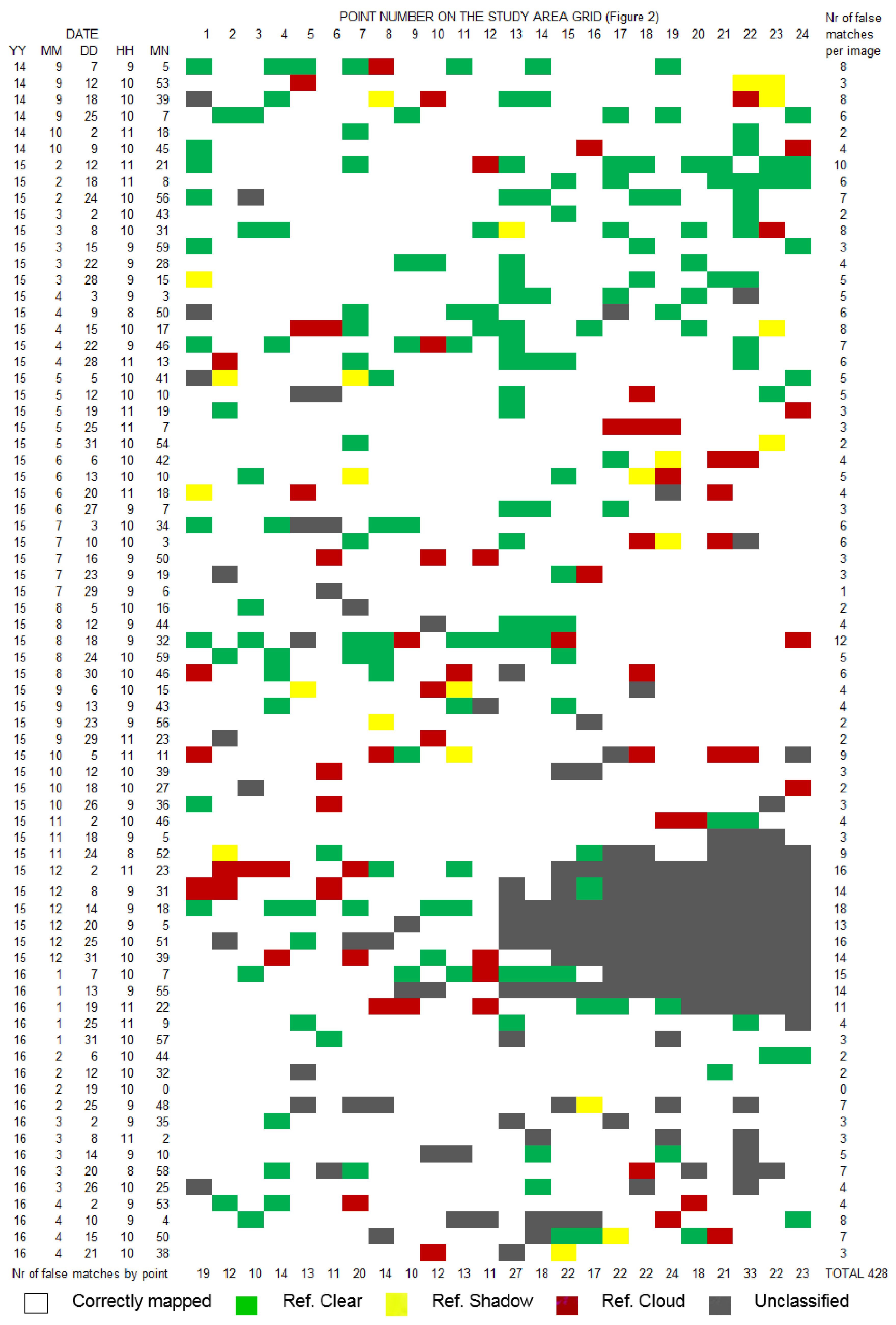
Thin clouds remained problematic to detect. When decreasing the cloud threshold of the visible bands to detect thin clouds, the number of false detections of built areas to cloud class increased. Because of the application of a grid, the reference points were located sporadically in the center or in the edges of the clouds and shadows. It would have been easier to detect the center of the clouds or shadows.

The ratio between blue and green detected shadows but thin mixed pixels shadows (one to two pixel wide) remained undetected. Part of the shadows were mixed with shallow water and dense coniferous forest. Cloud shadows on clouds were also problematic to detect. Sometimes the origin of the shadow is something else than cloud, for instance, in mountainous areas. However, this cannot be seen as a defect of the method because these areas also need special attention during analysis. For applications very sensitive to omitted shadows and clouds (e.g., model-based forest variable estimation), it is more desirable to reduce omissions as much as possible even at the cost of more false alarms. In optical satellite images, shadows are expected to appear in the vicinity of clouds along the sun angle direction [14]. A possibility to reduce omission of shadows adjacent to detected clouds would be to dilate cloud masks by several pixels along the sun angle direction. However, omitted shadows not contiguous with any cloud would require such a wide buffer around cloud masks that many clear pixels would be unnecessarily masked out, further increasing the false alarm rate.

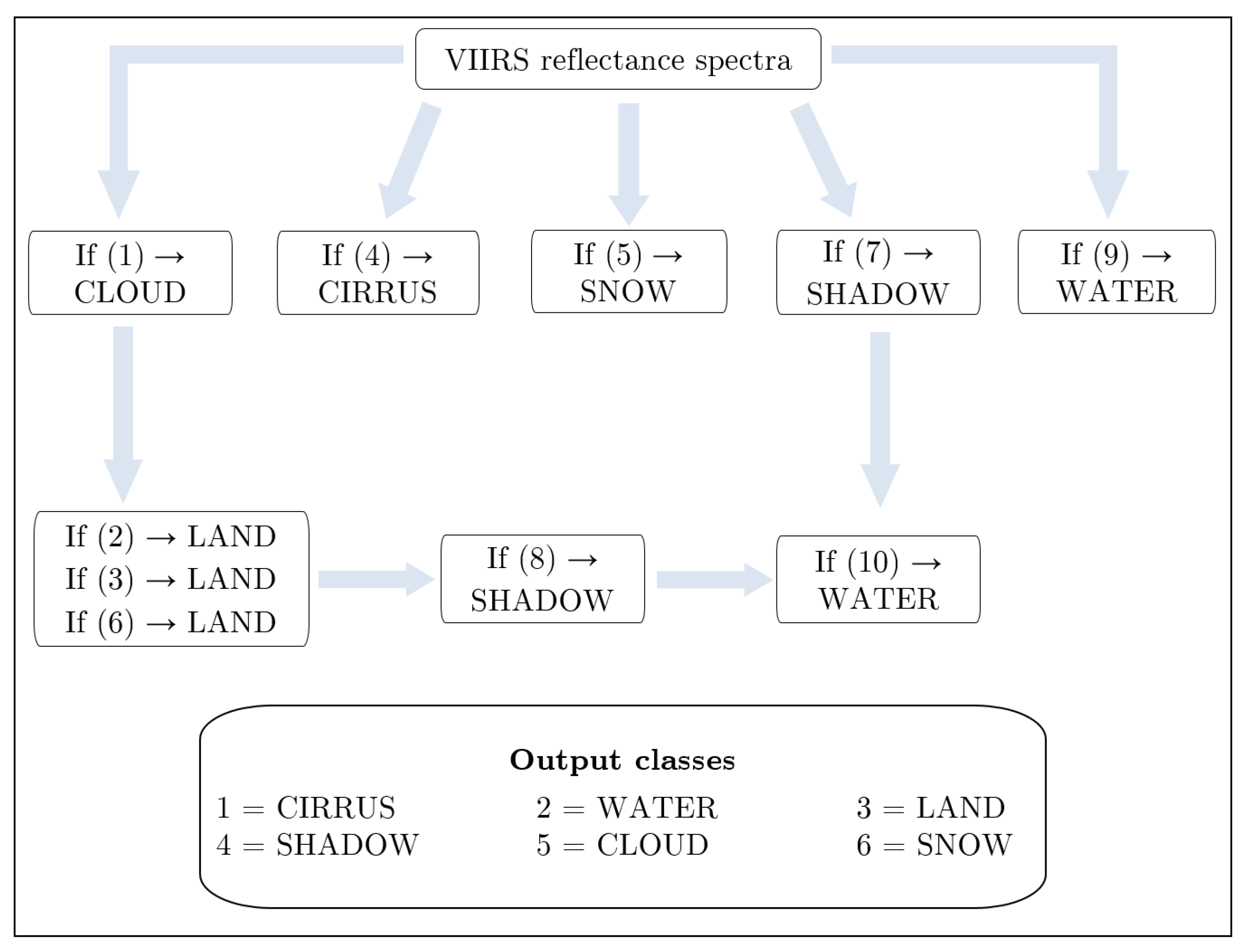
Because of a low sun angle, winter images were challenging in separation of snow and ice from the clouds. The snow index worked quite well, but part of the snow mixed with clouds. In winter images, the order of cirrus and snow detection affected the result. If snow and ice detection was performed after cirrus cloud detection, the snow detection found ice covered lakes from under the cirrus clouds. More generally, the threshold for the cirrus detection is subjective, and though the same threshold gave good results for all seasons’ images, some applications may need imagery with less cirrus cover removed. They are not visible in the visible bands, and so applications using only visible bands may use higher threshold for the cirrus detection. The subjective threshold can then be selected interactively from the cirrus band image. During winter season from end of November to end of January, the visual interpretation could not be done in the Northern part of Fennoscandia (with latitudes north of $65{}^{\circ }$) due to the low sun angle. In February 2015 a slightly bigger proportion of false alarms for clouds were observed in the latitudes north of about $68{}^{\circ }$ (Figure 8). This did not show in February 2016 results. The reason may be that in 2015 the thermal spring came one month earlier than in 2016 (according to the Finnish Meteorological Institute—http://www.fmi.fi) and there was a bigger amount of clear melted or nearly melted land pixels in the north. These pixels were wrongly assigned to cirrus or cumulus clouds and decreased the separation between clear land and cloud, which was the biggest mismatch in Table 3 with 120 occurrences.

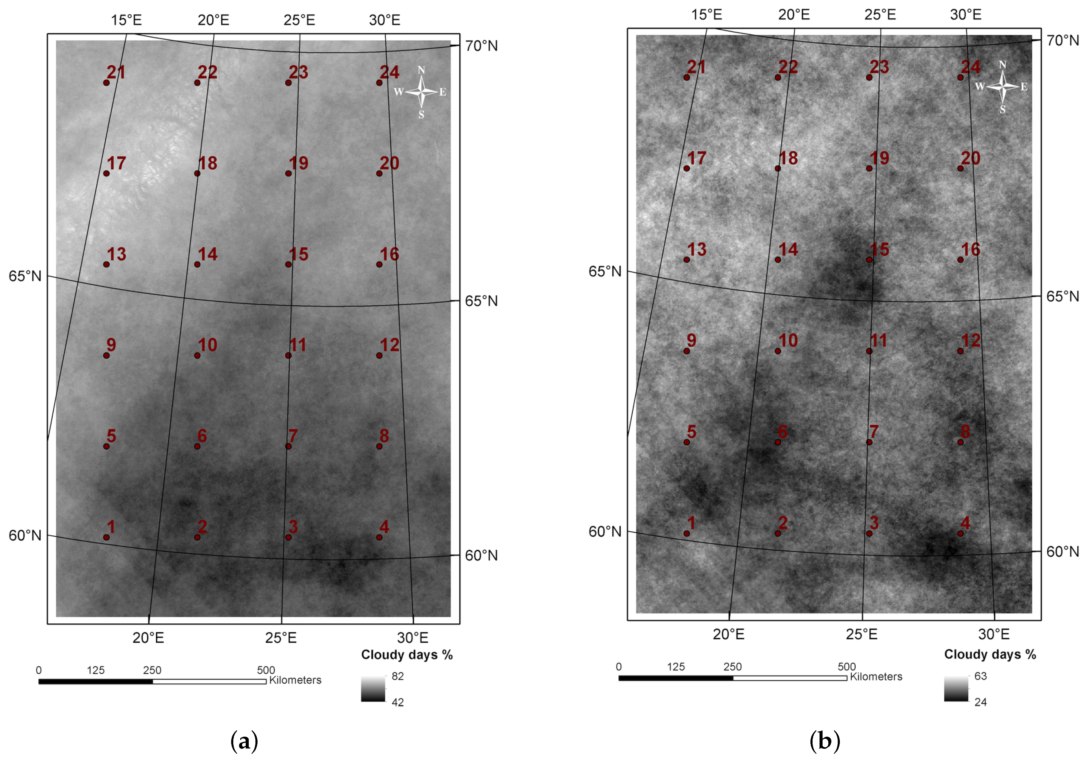
Pixel-wise percentage of cloudy days (Figure 8) were calculated from the 747 images based on the cloud and shadow masks. The percentage of cloudy days from the whole dataset in Figure 8a, which also includes winter images, showed snow and ice areas in northern Norway (north-west part of the image) to be more frequently covered by clouds. This can be an error in cloud interpretation or an indication of high cloud cover in high mountains with also snow or ice coverage during all seasons. In both images, the sea and big lakes areas were less cloudy than other areas. This was because some thin clouds and their shadows are difficult to separate from water, but also because cumulus clouds typically do not exist over sea areas. These statistics images also highlighted noise striping in the south-west corner of the area, which were due most probably to the scanning instrument or the pre-processing lines. Otherwise the statistics images did not show any systematic features that could be assigned to biases in the cloud computing algorithm.

The results of the proposed method can be compared to published results from other methods applied to VIIRS images in Northern Europe. For the proposed method, the correct detection rate of clouds was 94.2% and false alarms rate 11.1%. For the VIBCM method in Northern Europe area [4], a slightly higher correct detection rate was reported for clouds (94.5%), at the cost of a much larger false alarm rate (42.1%). However, the proposed method does not use thermal bands, yet reaches similar accuracies as the VCM and VIBCM methods, which makes it an interesting operational method for several sensors, including Sentinel-2. As an example, Figure 9 presents the result of cloud and shadow masking for a Sentinel-2 image acquired in June 2016 in Southern Finland, using the same method with corresponding bands from Sentinel-2 imagery.

The VIIRS dataset was quite challenging, with high latitude (sun angle effects), frequent snow/ice and cloud cover. Because of the coarse resolution, most shadows in VIIRS images were very small (2–3 pixels wide), and there were many mixed pixels.

The method used the green band with blue band in shadow ratio. This ratio increased in cloud shadows because shadow pixels are illuminated by the predominantly blue, diffuse sky radiation. In [7] the SWIR, NIR or red band was used instead of the green band to yield optimal results. The reason might be the different land cover types dominating the area. In the boreal study area used in this paper, forested and water areas dominated with high reflectance in green band. On the contrary, in bright built and desert areas, the red band reflectance is higher than in vegetated areas and might give better results.

6. Conclusions

A new method for cloud and shadow detection was developed for optical satellite images. Accuracy assessment was performed with visual reference data collected on 1752 points located in Fennoscandia, over 73 Suomi NPP VIIRS images selected between August 2014 to April 2016. When comparing the results on 73 VIIRS images with visually interpreted reference data, the method detected clouds with a 94.2% correct detection rate and 11.1% false alarm rate. These figures were at the same level as the state of the art from literature for cloud detection, however without using the thermal bands. For shadows, the correct detection rate was 36.1% and the false alarm rate was 82.7%. The test area in the boreal zone contained plenty of water and dense forest area which are challenging especially shadow detection methods. The method is stable in the sense that the same rules and thresholds could be applied to VIIRS images of all the seasons. Because the method does not use thermal bands, it can be applied to several optical sensors, including Sentinel-2. Also the future low resolution optical sensors for global near real time and climate change studies, like Sentinel-3 and the operative satellites following Suomi NPP, can benefit from this method.

References

1. Zhou, L.; Divakarla, M.; Liu, X. An overview of the Joint Polar Satellite System (JPSS) science data product calibration and validation. Remote Sens. 2016, 8. [Google Scholar] [CrossRef]
2. Vermote, E.; Justice, C.; Csiszar, I. Early evaluation of the VIIRS calibration, cloud mask and surface reflectance earth data records. Remote Sens. Environ. 2014, 148, 134–145. [Google Scholar] [CrossRef]
3. Hutchison, K.D.; Heidinger, A.K.; Kopp, T.J.; Iisager, B.D.; Frey, R.A. Comparisons between VIIRS cloud mask performance results from manually generated cloud masks of VIIRS imagery and CALIOP-VIIRS match-ups. Int. J. Remote Sens. 2014, 35, 4905–4922. [Google Scholar] [CrossRef]
4. Piper, M.; Bahr, T. A rapid cloud mask algorithm for Suomi NPP VIIRS Imagery EDRs. Int. Arch. Photogramm. Remote Sens. Spat. Inf. Sci. 2015, XL-7/W3, 237–242. [Google Scholar] [CrossRef]
5. Hall, D.K.; Riggs, G.A. Normalized-Difference Snow Index (NDSI). In Encyclopedia of Snow, Ice and Glaciers; Singh, V.P., Singh, P., Haritashya, U.K., Eds.; Springer: Dordrecht, The Netherlands, 2011; pp. 779–780. [Google Scholar]
6. Valocvin, F. Snow/Cloud Discrimination; Technical Report AFGL-TR-76-0174, ADA 032385; Air Force Geophysics Laboratory: Hanscom Air Force Base, MA, USA, 1976.
7. Luo, Y.; Trishchenko, A.P.; Khlopenkov, K.V. Developing clear-sky, cloud and cloud shadow mask for producing clear-sky composites at 250-m spatial resolution for the seven MODIS land bands over Canada and North America. Remote Sens. Environ. 2008, 112, 4167–4185. [Google Scholar] [CrossRef]
8. Gao, B.C.; Goetz, A.F.H.; Wiscombe, W.J. Cirrus cloud detection from airborne imaging spectrometer data using the 1.38 μm water vapour band. Geophys. Res. Lett. 1993, 20, 301–304. [Google Scholar] [CrossRef]
9. Gao, B.C.; Kaufman, Y.J.; Tanre, D.; Li, R.R. Distinguishing tropospheric aerosols from thin cirrus clouds for improved aerosol retrievals using the ratio of 1.38-µm and 1.24-µm channels. Geophys. Res. Lett. 2002, 29. [Google Scholar] [CrossRef]
10. Lavanant, L.; Marguinaud, P.; Harang, L.; Lelay, J.; Péré, S.; Philippe, S. Operational cloud masking for the OSI SAF global METOP/AVHRR SST product. In Proceedings of the 2007 EUMETSAT Meteorological Satellite Conference, Amsterdam, The Netherlands, 24–28 September 2007; pp. 24–28. [Google Scholar]
11. Zhu, Z.; Wang, S.; Woodcock, C.E. Improvement and expansion of the Fmask algorithm: Cloud, cloud shadow, and snow detection for Landsats 4–7, 8, and Sentinel 2 images. Remote Sens. Environ. 2015, 159, 269–277. [Google Scholar] [CrossRef]
12. Dozier, J. Spectral signature of alpine snow cover from the landsat thematic mapper. Remote Sens. Environ. 1989, 28, 9–22. [Google Scholar] [CrossRef]
13. Metsämäki, S.; Pulliainen, J.; Salminen, M.; Luojus, K.; Wiesmann, A.; Solberg, R.; Böttcher, K.; Hiltunen, M.; Ripper, E. Introduction to GlobSnow Snow Extent products with considerations for accuracy assessment. Remote Sens. Environ. 2015, 156, 96–108. [Google Scholar] [CrossRef]
14. Zhu, Z.; Woodcock, C.E. Object-based cloud and cloud shadow detection in Landsat imagery. Remote Sens. Environ. 2012, 118, 83–94. [Google Scholar] [CrossRef]
15. Hagolle, O.; Huc, M.; Pascual, D.V.; Dedieu, G. A multi-temporal method for cloud detection, applied to FORMOSAT-2, VENµS, LANDSAT and SENTINEL-2 images. Remote Sens. Environ. 2010, 114, 1747–1755. [Google Scholar] [CrossRef] [Green Version]
16. Zhu, Z.; Woodcock, C.E. Automated cloud, cloud shadow, and snow detection in multitemporal Landsat data: An algorithm designed specifically for monitoring land cover change. Remote Sens. Environ. 2014, 152, 217–234. [Google Scholar] [CrossRef]
17. Rahman, H.; Dedieu, G. SMAC: A simplified method for the atmospheric correction of satellite measurements in the solar spectrum. Int. J. Remote Sens. 1994, 15, 123–143. [Google Scholar] [CrossRef]
18. Andersson, K. AOD Correction and Cloud Masking; Technical Report; VTT Technical Research Centre of Finland Ltd.: Espoo, Finland, 2015. [Google Scholar]
Figure 1. (a) Study area, Study area with reference grid points in red; (b) VIIRS samples (reference point 11), A set of VIIRS samples with the surroundings for the visual interpretation of clouds and non-clouds. The square images in (b) are the VIIRS samples at the reference point 11 from (a), for dates ranging from 7 September 2014 (top-left square) to 5 August 2015 (bottom right square). The squares are RGB composite images with reflectance bands 0.67 μ m, 0.555 μ m and 0.445 μ m as Red, Green and Blue channel respectively.
Remotesensing 09 00806 g001
Figure 2. Cloud and shadow detection flow chart. The output mask is initialised to land class (clear pixel). Rules are successively evaluated along the paths shown with blue arrows. When a rule is false, the output class for the pixel remains unchanged. When a rule is true, the output is assigned to the class associated with that rule (after the black arrow → in the corresponding box).
Remotesensing 09 00806 g002
Figure 3. A Suomi NPP VIIRS image of 5 August 2014, at 09:28 a.m. (a) SWIR colour composite, RGB composite from 3.7 μ m, 2.2 μ m and 1.6 μ m reflectance; (b) Natural colours, Natural colour image from 0.672 μ m, 0.555 μ m and 0.490 μ m reflectance; (c) Cloud/shadow result, Cloud and shadow detection result.
Remotesensing 09 00806 g003
Figure 4. A Suomi NPP VIIRS image of 20 October 2014, at 10:39 a.m. (a) SWIR colour composite, RGB composite from 3.7 μ m, 2.2 μ m and 1.6 μ m reflectance; (b) Natural colours, Natural colour image from 0.672 μ m, 0.555 μ m and 0.490 μ m reflectance; (c) Cloud/shadow result, Cloud and shadow detection result.
Remotesensing 09 00806 g004
Figure 5. A Suomi NPP VIIRS image of 25 April 2015, at 10:28 a.m. (a) RGB from 3.7 μ m, 2.2 μ m and 1.6 μ m reflectance. (a) RGB composite from 3.7 μ m, 2.2 μ m and 1.6 μ m reflectance. (b) Natural colour image from 0.672 μ m, 0.555 μ m and 0.490 μ m reflectance. (c) Cloud and shadow detection result. (a) SWIR colour composite; (b) Natural colours; (c) Cloud/shadow result.
Remotesensing 09 00806 g005
Figure 6. A Suomi NPP VIIRS image of 16 February 2016, at 10:57 a.m (a) SWIR colour composite, RGB composite from 3.7 μ m, 2.2 μ m and 1.6 μ m reflectance; (b) Natural colours, Natural colour image from 0.672 μ m, 0.555 μ m and 0.490 μ m reflectance; (c) Cloud/shadow result, Cloud and shadow detection result.
Remotesensing 09 00806 g006
Figure 7. Distribution of correct and false matches by date (y-axis) and by reference point index (x-axis).
Remotesensing 09 00806 g007
Figure 8. Cloudy days percentages computed on the whole Suomi NPP VIIRS dataset (a) and on summertime images (b). The numbered points from 1 to 24 are the visually interpreted reference points. (a) All VIIRS images (741); (b) Summertime images only (145).
Remotesensing 09 00806 g008
Figure 9. Extract of Sentinel-2 image of 29 June 2016, Southern Finland. (a) Natural colour image from 0.672 μ m, 0.555 μ m and 0.490 μ m reflectance. High clouds on land and sea areas are shown in magenta, low clouds in orange. (b) Cloud and shadow detection result. (a) Natural colour image; (b) Cloud/shadow result.
Remotesensing 09 00806 g009