Article

Underlying Topography Estimation over Forest Areas Using High-Resolution P-Band Single-Baseline PolInSAR Data

School of Geosciences and Info-Physics, Central South University, Changsha 410083, China
*
Authors to whom correspondence should be addressed.
Remote Sens. 2017, 9(4), 363; https://doi.org/10.3390/rs9040363
Submission received: 19 February 2017 / Revised: 26 March 2017 / Accepted: 9 April 2017 / Published: 12 April 2017
(This article belongs to the Special Issue Calibration and Validation of Synthetic Aperture Radar)

Abstract

:
This paper discusses the potential and limitations of high-resolution P-band polarimetric synthetic aperture radar (SAR) interferometry (PolInSAR) in underlying topography estimation over forest areas. Time-frequency (TF) analysis in the azimuth direction is utilized to separate the ground scattering contribution from the total PolInSAR signal, without the use of any physical model, because the P-band PolInSAR data have a significant penetration depth and sufficient observation angle interval. To achieve this goal, a one-dimensional polynomial fitting (PF) method is proposed for correcting the residual motion error (RME). The Krycklan catchment test site, which is covered with pine forest, was selected to test the performance of the digital elevation model (DEM) inversion. The results show that the PF method can correct the RMEs for the sub-look interferograms well. When compared to the existing line-fit method, the TF+PF method can provide a more accurate DEM (the accuracy is improved by 26.9%). Moreover, the performance of the DEM inversion is free from the random-volume-over-ground assumption.

Graphical Abstract

1. Introduction

Digital elevation models (DEMs) play an important role in many applications, such as geohazard prediction [1], resource exploration, and flood inundation simulation [2]. In providing all-weather and global coverage monitoring, interferometric synthetic aperture radar (InSAR) has been demonstrated to be a promising tool for topographic mapping [3,4]. However, despite the fact that InSAR working in the microwave band can penetrate the forest layer to a certain degree, the derived elevation is usually somewhere between the elevation of the forest canopy and the ground surface, as it is still contaminated by forest height signals [2,5].
Polarimetric interferometric SAR (PolInSAR) can distinguish the phase centers of multiple targets in a common cell over a forest area [6]. This provides the possibility to separate ground scattering contributions from canopy scattering contributions. The underlying topography in forest areas can then be measured with the ground interferometric phase or by subtracting the forest height from an existing digital surface model (DSM). Several approaches have been proposed to estimate the ground scattering contributions [7,8,9,10,11,12]. Among them, the inversion method based on the random-volume-over-ground (RVoG) model has been widely used, as it can model a forest with few parameters and connect the PolInSAR complex coherences with the forest biophysical parameters [7,13,14]. In the RVoG model, the forest is assumed to be a homogeneous random volume. Based on this assumption, the extinction is independent of the polarization. As a result, the complex coherences corresponding to different polarizations follow a straight line in the complex plane, and the ground interferometric phase can be estimated with the line-fit method [8], which has been widely applied in forest height inversion in the X, C, and L bands over different forest types [15,16,17]. However, the ground interferometric phases derived from the X, C, and L bands are still biased because of their limited penetration depths. The P-band SAR system provides deeper sampling of the forest layer than the higher-frequency SAR systems, which allows us to measure the phase centers closer to the ground surface. However, the RVoG assumption is not fulfilled in the P-band, as the main scatterers in the forest are large-scale forest structural elements (e.g., branches and trunks), which present heterogeneity in the whole forest height extent [18]. The accuracy of the ground interferometric phase is affected by the orientation effect when the line-fit method is adopted to calculate the ground phase. Hence, the oriented-volume-over-ground (OVoG) model [19,20] seems to be more appropriate for depicting the scattering process of the P-band. However, the ground phase cannot be estimated with the OVoG model in the single-baseline configuration because of the underdetermined problem [20,21,22]. Garestier et al. [23,24,25] proposed a time-frequency (TF) approach that searches for the pure ground scattering contribution by changing the observation angle in the azimuth direction. The TF method, which is independent of a physical model or assumption, has been applied to OVoG model inversion for separating the ground scattering contributions in forest height inversion [24]. In such an application, the effect of the residual motion error (RME) [26,27] on the forest height can be omitted because the different polarimetric interferograms have a common RME, which can be counteracted in the phase difference based forest height inversion. However, if the TF method is applied to extract the underlying DEM, the RME must be carefully considered. The reason for this is that it is difficult to obtain accurate positioning information for every sub-look, which affects the time-frequency analysis and limits the accuracy of the DEM.
This study proposes underlying DEM inversion for forest areas based on a refined TF method for single-baseline P-band PolInSAR data to overcome the above limitation. After sub-look decomposition and interferometry, a polynomial fitting (PF) method is proposed for fitting the RME of each sub-look interferogram along the range direction. The corrected sub-look interferograms are then used to detect the ground phase. After interferogram filtering and phase unwrapping, the ground phase is converted to ground height by the linear relationship between the ground phase and the ground height. In order to test the performance of the refined TF method, a boreal forest in the Krycklan catchment was investigated. The corresponding P-band repeat-pass PolInSAR data were collected in the BioSAR 2008 campaign [28]. Finally, this paper discusses the effect of the RME on the DEM inversion. Moreover, a simple RVoG/non-RVoG test based on the differences of the DEMs generated by the line-fit and TF methods is carried out. Based on this, a quantitative analysis of the DEM errors over the RVoG and non-RVoG areas is conducted.

2. Underlying Topography Estimation over Forest Areas from PolInSAR

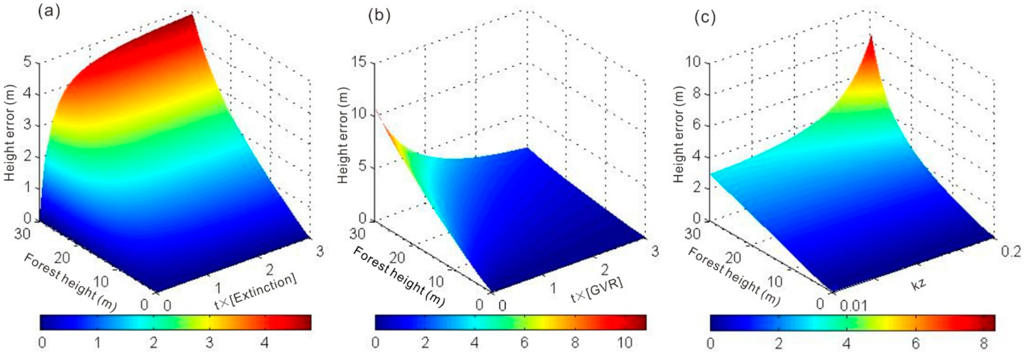
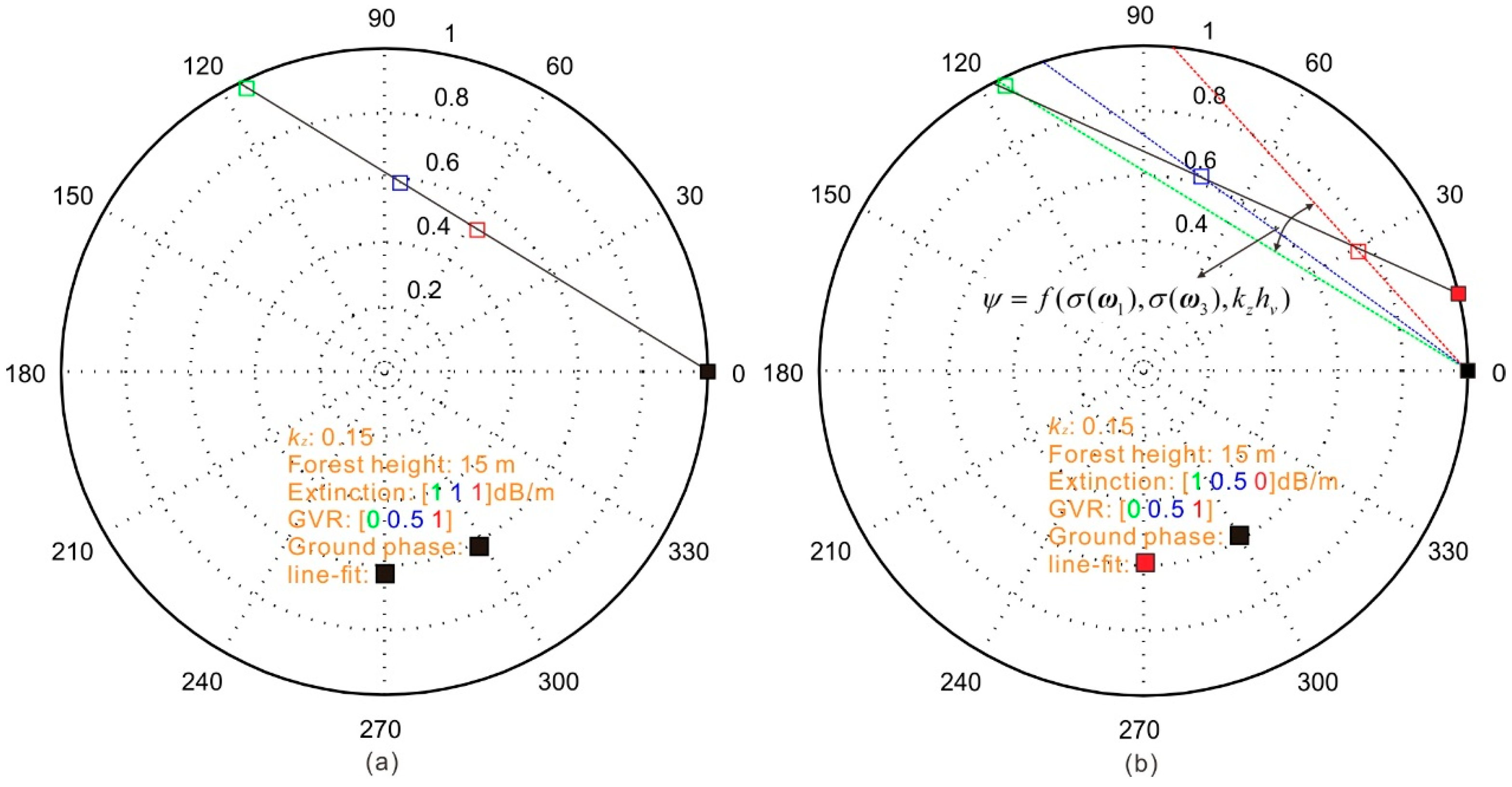
2.1. Limitations of RVoG-Based Ground Phase Inversion

The RVoG model describes forest as a homogeneous random volume over an impenetrable ground surface [7]. The complex coherence γ ( ω ) corresponding to the polarization ω is defined as [7]
γ ( ω ) = e i φ 0 γ v + μ ( ω ) 1 + μ ( ω )
where φ 0 is the ground interferometric phase directly related to the underlying topography. μ ( ω ) denotes the ground-to-volume ratio (GVR), which changes with the polarization ω . γ v represents the pure volume decorrelation, and is a function of the vegetation height h v , the extinction σ , the vertical wavenumber k z , and the incidence angle θ [7]:
γ v = 2 σ ( e ( 2 σ h v / cos θ + i k z h v ) 1 ) ( 2 σ + i k z cos θ ) ( e 2 σ h v / cos θ 1 )
In the RVoG model, since the volume layers are assumed to be homogeneous, they are characterized by polarization-dependent extinction. Therefore, different polarization coherences have the same pure volume decorrelation γ v . In such a situation, according to Equation (1), the complex coherences associated with different polarizations follow a straight line in the complex plane, and locate between the pure ground and volume coherences. Without considering the effect of temporal decorrelation, the phase center of the polarization ω is equal to the ground interferometric phase φ 0 when μ ( ω ) tends to + . Thus, the ground interferometric phase can be identified through the intersections of the straight line and the complex unit circle. To clarify this, a PolInSAR configuration was simulated with Equations (1) and (2) as follows: a 20-m forest height with a 1-dB/m extinction, a ground phase of 0 rad, a GVR spectrum with μ ( ω 1 ) : μ ( ω 2 ) : μ ( ω 3 ) = 0 : 0.5 : 1 , and a vertical wavenumber of 0.15. Three different complex coherences were simulated and are shown in Figure 1a. As the figure shows, the three simulated complex coherences are on a straight line. In addition, one of the two intersections of the line and the complex unit circle is the pure ground coherence, whose angle is equal to the ground interferometric phase.
The effect of polarizations with different extinctions (as described by the OVoG mode) on the line-fit method was then considered. Differing from the RVoG case, the extinctions of the three polarizations were set as σ ( ω 1 ) : σ ( ω 2 ) : σ ( ω 3 ) = 1 : 0.5 : 0 dB/m. With Equations (1) and (2), three complex coherences were calculated and are shown in Figure 1b. The coherence for each polarization can only move up and down along its own line. In such a case, if the line-fit method is adopted, the estimated ground phase is biased, as shown by the black line in Figure 1b. Furthermore, there is an angle ψ between the green and red lines, which correspond to the two polarizations with maximal and minimal extinctions, respectively. This angle is a function of σ ( ω 1 ) , σ ( ω 3 ) , and k z h v [20]. With the decreasing angle ψ , the OVoG model approaches the RVoG model. Based on this, the ground interferometric phase derived by the line-fit method may not significantly deviate from the true value. To better understand the relationships between the ground interferometric phase bias and the GVR, the extinction and the vertical wavenumber were investigated since they affect the angle ψ . Three simulation experiments were conducted with the parameters listed in Table 1. t × (1:0.5:0) dB/m was used to generate a series of extinction spectra. In other words, the narrowest extinction spectrum can be obtained when t = 0, and the widest extinction spectrum when t = 3. In the same way, a series of GVR spectra were generated. As Figure 2 shows, the ground height error derived by the line-fit method varies with the extinction, the GVR, and the vertical wavenumber. It can be concluded that the ground height error increases with the increasing forest height, the widening extinction spectrum, and the vertical wavenumber, but decreases with the widening GVR spectrum.
Based on the above analysis, if the angle ψ is small enough, the ground height error induced by the line-fit procedure can be acceptable, as used in agriculture underlying topography inversion [22]. However, in practice, it is usually difficult to obtain the prior information of the angle ψ and a threshold of the angle ψ , which allows for the estimation of the ground phase using the line-fit method. The eccentricity of the coherence boundary [29] may be a potential tool for solving this problem. Once the relationship between the angle ψ and the ground phase error caused by the line-fit method are known, it is possible to reduce the corresponding error by selecting a small k z , as revealed in Figure 2c. This may be useful for forest height inversion with the OVoG model. However, this is not a good strategy for DEM inversion because a small k z corresponds to a large 2π-height ambiguity and is less sensitive to the terrain variation [20]. Compared with higher-frequency SAR signals, the P-band signal has a larger penetration depth, so it can capture more ground scattering contributions in all polarizations. This, as shown in Figure 2b, is beneficial to the DEM inversion. However, bias still occurs since the extinctions of the different polarizations are different in the P-band, because of the orientation effect [24]. Based on the above analysis, it is clear that it is necessary to propose an approach which is free from the RVoG assumption, to estimate the ground interferometric phase from P-band single-baseline PolInSAR data.

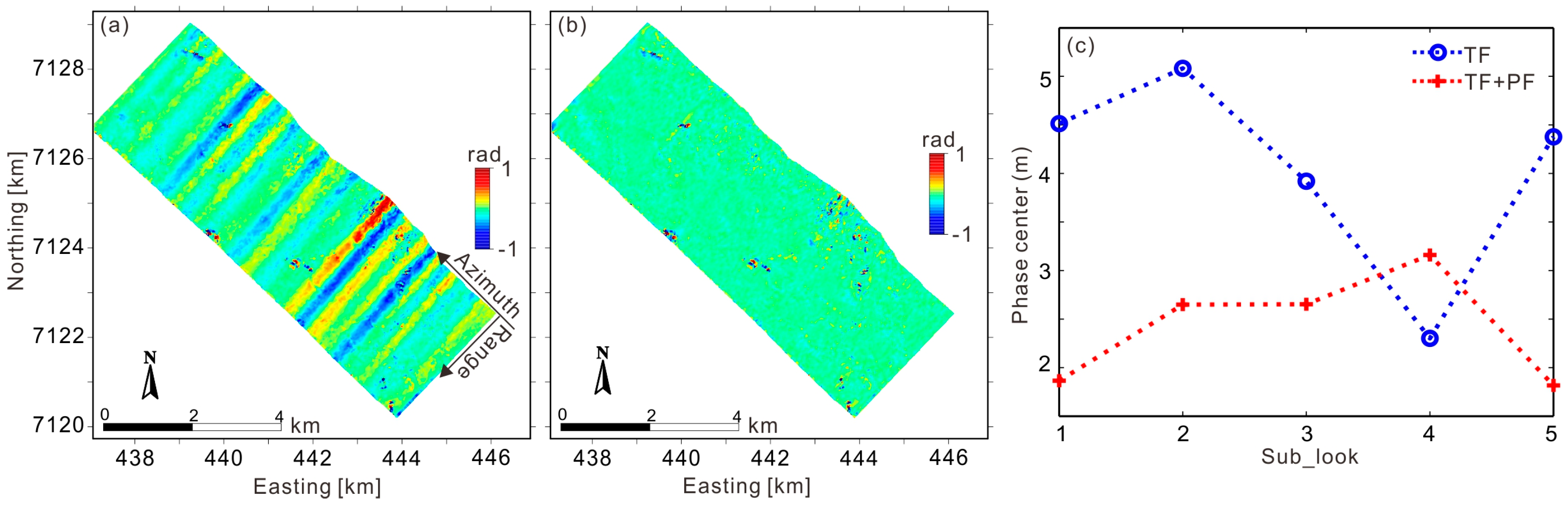
2.2. Ground Phase Inversion by the TF Method

The impulsion-compression technique is utilized to achieve a high resolution in the SAR imaging process. This process depends on the fact that the relative movement between the observed target and the platform induces a time-varying Doppler frequency fd, which is related to the azimuth position of the target and its distance to the platform. Therefore, a target in a resolution cell can be seen from a time-varying observation angle φ during the azimuthal integration, which provides a way to obtain the ground scattering contribution contaminated by the minimal volume scattering contribution. Consequently, a phase center closer to the underlying topography can be selected from the obtained sub-look images. The observation angle can be expressed by a function of the Doppler bandwidth fd, the radar wavelength λ , and the platform velocity vp [23,24,26]
φ = arcsin ( f d λ 2 v p )
The obtained Doppler bandwidth is proportional to the observation angle variation interval Δ φ , but is inversely proportional to the azimuth resolution δ a z [23,24,26]
Δ φ = λ 2 δ a z
Figure 3a shows the frequency spectral filtering effect on the azimuth observation angle. Three overlapped sub-looks are represented by the red, green, and blue dashed lines, and only the red and blue sub-looks have independent frequency spectra. The azimuth observation angle intervals of the three sub-looks, as shown in the lower part of the figure, are the same since the three sub-looks have the same bandwidths.
P-band SAR data with a high resolution can be used for the TF investigation of the scatterer physical properties because of the large Δ φ . Moreover, for the P-band signal, the main scattering targets are large-scale trunks with different spatial distributions and densities when “seen” from different observation angles by the SAR sensor. Hence, the SAR signals received from different observation angles contain different-level volume scattering contributions. Furthermore, previous research has demonstrated that the HH polarimetric signal in the P-band is sensitive to the ground and double-bounce scattering in the forest [24]. Thus, the ground can be “seen” more or less directly by the SAR sensor when the observation angle varies.
Using interferometry, the obtained sub-look images can be converted to sub-look interferograms. The phase centers associated with the obtained sub-look interferograms can then be investigated and the ground phase can be estimated. Before doing this, it is very important to remove the RME from every sub-look interferogram. The reason for this is that each sub-look interferogram has different RME, as shown in Figure 3b. As a result, the phase center of the sub-look interferogram cannot be exactly interpreted due to the interference of the RME. Hence, in the following section, this paper introduces how to remove the RME.

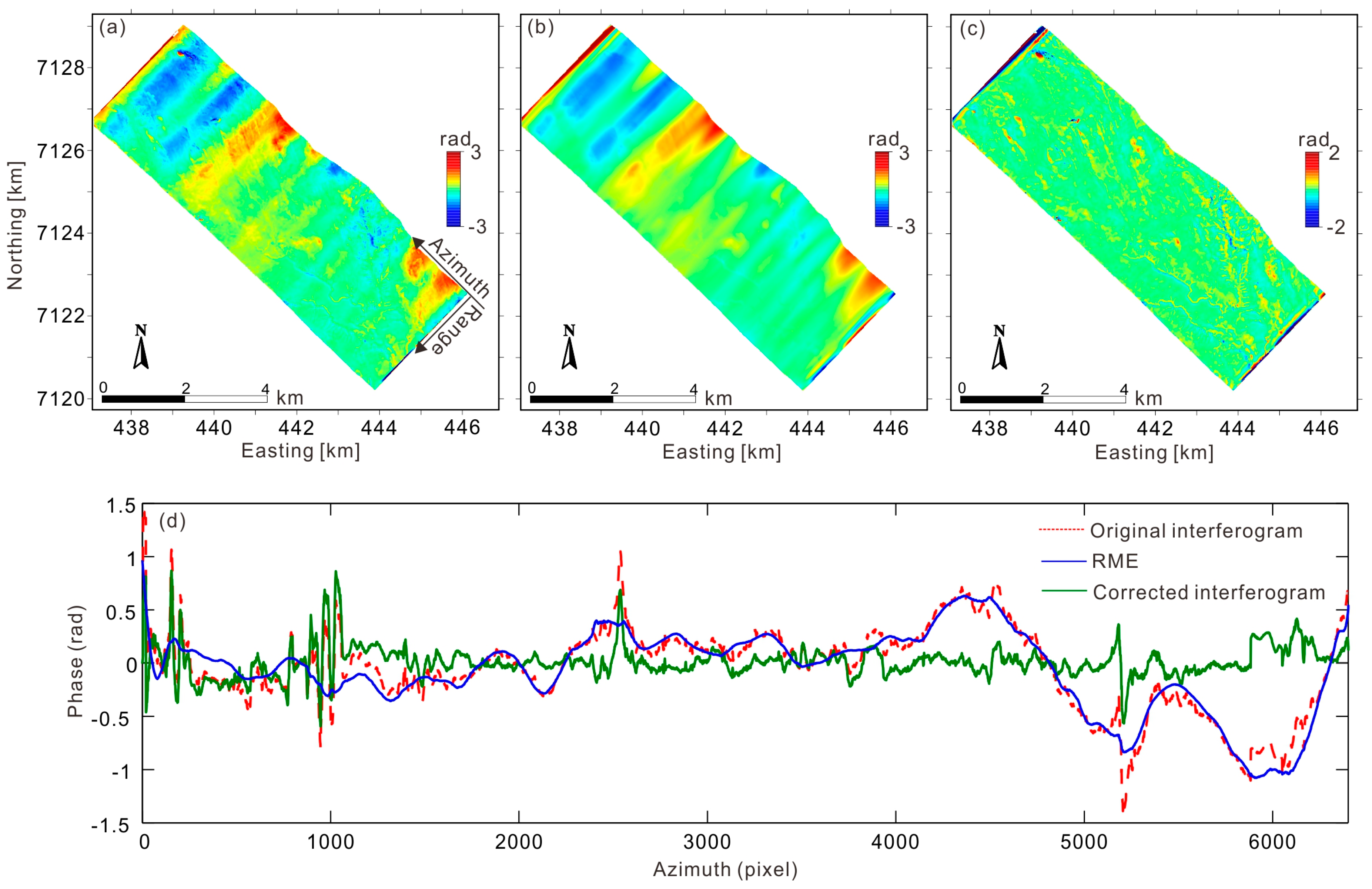
2.3. RME Correction by the PF Method

In airborne interferometry, several works have addressed compensating the RME for single-baseline InSAR or multi-baseline InSAR data [30,31,32]. Among the different methods, the multisquint processing technique has been widely used for mitigating the RME for single-baseline InSAR data [31,32]. This method needs to calculate the derivative of the RME by the differences of the sub-look interferograms [26]. However, in a forest area, different sub-look interferograms will have different penetration depths, which limits the estimation of the RME derivative [24,26]. Moreover, the multisquint processing technique has been designed for correcting the RME of the full-resolution interferogram, and it cannot completely remove the RME for every sub-look interferogram. As a result, the phase center for every sub-look interferogram cannot be accurately interpreted. In the following, this study introduces the PF method to remove the RME for every sub-look interferogram.
After sub-look decomposition and interferometry, several sub-look interferograms can be generated. For the ith sub-look interferogram, the interferometric phase φ int i is composed of
φ int i = φ f l a t i + φ t o p o i + φ f o r e s t i + φ n o i s e i
where φ f l a t i and φ t o p o i are the flat-earth phase and topography phase, respectively. φ f o r e s t i is the phase caused by the forest height, and φ n o i s e i is the random error phase. In order to detect the RME, differential interferometry is separately performed for every sub-look interferogram. To achieve this, φ t o p o i can be calculated by the baseline parameters and the ground height h [33]:
φ t o p o = 4 π B cos ( θ α ) λ R 1 sin ( θ ) h
where B and α are the total baseline length and the baseline tilt angle, which are both calculated with the orbit state parameters. R 1 is the slant range of the master image, and θ is the incidence look angle, which is determined by the slant range R 1 and the platform altitude above ground. λ is the wavelength of the SAR signal. The flat-earth phase can be removed by [33]:
φ f l a t = 4 π B cos ( θ α ) λ R 1 tan ( θ ) ( R 2 R 1 )
where R2 is the slant range of the slave image. However, due to the unknown time-varying baseline error, φ f l a t i and φ t o p o i cannot be preciously calculated. As a result, the differential interferometric phase φ d i f f i can be expressed as:
φ d i f f i = φ R M E i + φ t o p o i + φ f o r e s t i + φ n o i s e i
where φ t o p o i is the phase caused by the input DEM error, which is independent of the sub-look. φ R M E i is the RME, which is composed of the residual flat-earth phase and the residual topography phase. In order to obtain a reliable forest phase center φ f o r e s t i and perform a good TF analysis between the sub-looks, it is necessary to remove the RME from every sub-look interferogram.
Since the baseline error is time-varying, which results in phase undulations along the azimuth direction, it is impossible to predefine a linear or high-order plane model to fit the RME, as used in spaceborne interferometry [34]. However, in the range direction, the errors of the baseline length and slant range are scaled by the incidence angle and ground height, which present a definite trend, as described by Equations (6) and (7). Based on this, this study proposes a one-dimensional polynomial model to fit the RME φ R M E ( x , y ) (x, y are the slant range and azimuth coordinates, respectively) along the range direction
φ R M E ( x , y ) = j = 0 n a j y j + a h h
where n is the order of the polynomial. a i and a h are the unknown coefficients, which can be estimated by least-squares estimation, as described in [34].
Before performing the PF process, using wavelet decomposition to remove some components of φ t o p o i , φ f o r e s t i , and φ n o i s e i which have shorter wavelengths than the RME [35] is recommended because these components can contaminate the fitting result of Equation (9). For this purpose, identifying the decomposition scale is critical, since the RME wavelength is unknown. To overcome this limitation, firstly, the root-mean-square error (RMSE) of the differential interferogram φ d i f f decomposed at scale J is defined as [36]
R M S E J = x = 1 , y = 1 m , n ( φ d i f f ( x , y ) φ ^ d i f f J ( x , y ) ) 2 / m n
where φ ^ d i f f J ( x , y ) represents the low-frequency component at decomposition scale J. Next, the change ratio R R M S E J of the RMSE is defined by [36]
R R M S E J = R M S E J + 1 / R M S E J
When the R R M S E J approaches 1, this means that the high-frequency components have been removed because the low-frequency components at decomposition scale J and J + 1 are approximate, and the decomposition scale can be set as J.

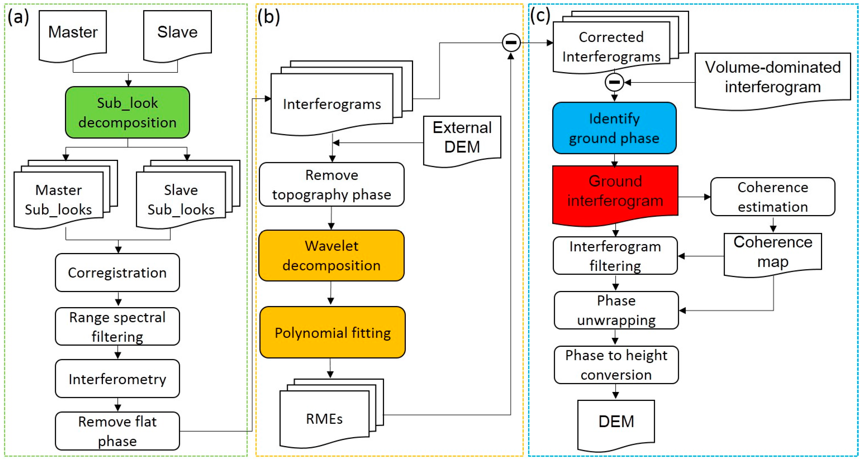
2.4. Underlying Topography Generation over Forest Areas with the TF+PF Method
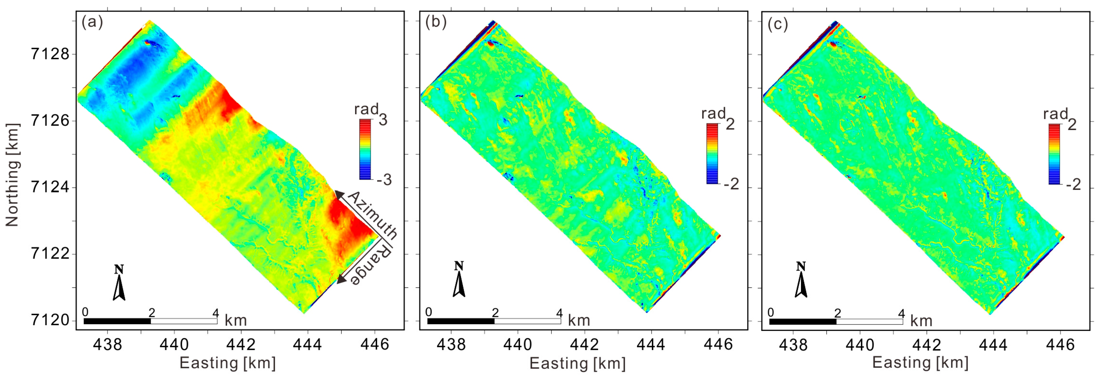
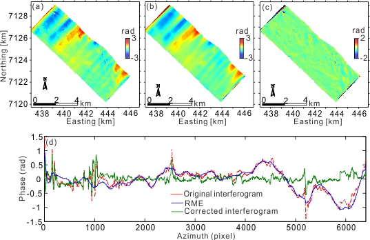
Finally, DEM inversion based on the TF+PF method is performed as described in Figure 4. The entire inversion framework is composed of (a) sub-look interferogram generation, (b) RME removal for every sub-look interferogram, and (c) DEM generation. For every part, there are several main procedures that should be noted:
(a)
In the sub-look interferogram generation, five sub-look images of equivalent resolution with 50% overlap are generated by Fourier transform filtering in the azimuth direction, while the range keeps the full resolution. More sub-look images can also be generated, but the experiments undertaken in this study showed that more sub-looks do not result in a significant difference for the DEM inversion;
(b)
For the RME removal, as adopted in [35], wavelet decomposition is performed using the Coiflet wavelet family of order 5, at a decomposition scale ranging from 1 to 10. Based on Equations (10) and (11), the optimal decomposition scale can be identified. The three-order (n = 3) polynomial in Equation (9) is then applied to fit the RME. The selection of the polynomial order is empirical. Although, in theory, a higher-order polynomial can fit the RME better, it is more sensitive to the residual components of φ t o p o i , φ f o r e s t i , and φ n o i s e i . Therefore, the three-order polynomial is a compromise between the fitting accuracy and the ability to resist error;
(c)
In the DEM generation, to identify the optimal ground phase, for every pixel, we find the sub-look whose interferometric phase has the largest difference with the interferometric phase of the volume-dominated polarization. Then, to improve the phase signal, the ground phase is filtered with a modified Goldstein filter [37]. Next, the filtered phase is unwrapped with the minimum cost flow (MCF) method [38]. Finally, the ground height can be obtained by the linear function of the ground phase and the vertical wave number [33].

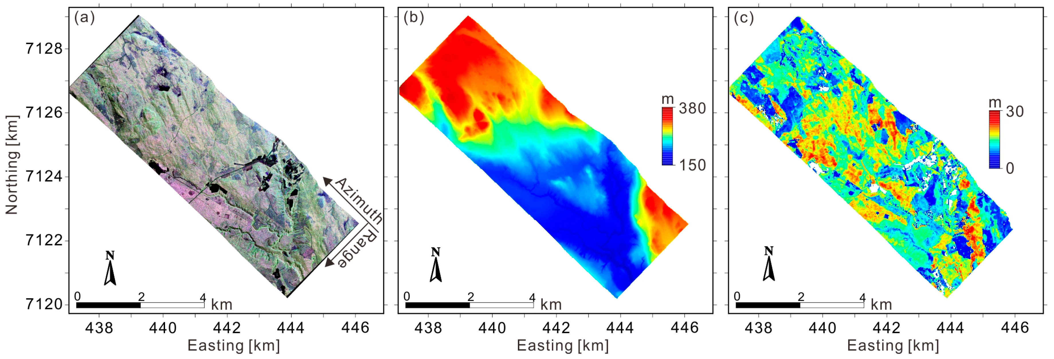
3. Test Sites and Data Sets

The test site is located in the Krycklan catchment, Sweden, where the dominant tree species are spruce, pine, and birch. The tree height ranges from 0 to 30 m in this area, and the ground elevation varies from 150 to 380 m above sea level. P-band polarimetric SAR (PolSAR) data for this test site were acquired by the German Aerospace Center’s (DLR) E-SAR airborne system in a repeat-pass configuration in the framework of the European Space Agency (ESA) BioSAR 2008 campaign [28]. Figure 5a shows the PolSAR image on the Pauli basis. The forest regions appear green due to the significant volume scattering contribution. The forest stand boundaries are clear in these high-resolution SAR images. The bare and water regions appear dark in the SAR intensity image since specular backscattering is observable. Two PolSAR images were selected for the interferometric process. The parameters of the interferometric pair are given in Table 2. Topography-dependent motion compensation had already been undertaken by the DLR. In addition, the DEM and forest height measured by light detection and ranging (LiDAR) in 2006, as shown in Figure 5b,c, were resampled to the SAR image resolution and taken as reference data. In spite of the forest height variation between 2006 and 2008, previous work [28] has indicated that the LiDAR-derived forest height in 2006 can be regarded as the reference data for the SAR data acquired in 2008.

4. Results and Analysis
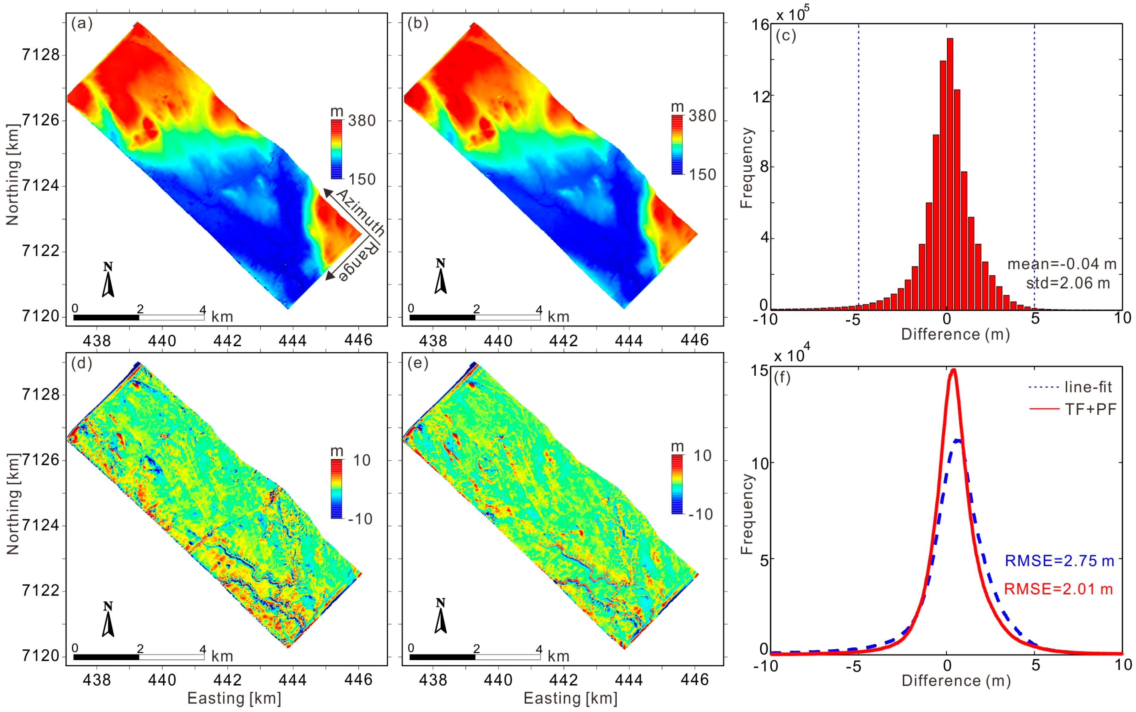
4.1. DEM Results

The TF+PF DEM inversion was conducted according to the process shown in the flowchart in Figure 4. In the RME removal process, the LiDAR-derived DEM was used to simulate the topography phase. As a comparison, the line-fit method was also used to generate a DEM. Before performing the line-fit process, the PF method was used to remove the RME from the full-resolution interferogram. The final DEM results are displayed in Figure 6a,b for the line-fit and TF+PF methods, respectively. It can be observed that the two derived DEMs present similar topographic patterns, with elevation values ranging from 150 to 380 m. Figure 6c shows the histogram of the difference of the line-fit and TF+PF DEMs. It can be observed that the differences mainly distribute between −5 and 5 m. Quantitatively, the global mean value for the differences is −0.04 m (with one standard deviation (std) = 2.06 m). The differences with respect to the LiDAR DEM are shown in Figure 6d,e, respectively. Clearly, the DEM derived by the line-fit method has a larger error than that of the TF+PF method. In particular, for the far-range region, it is noted that the line-fit DEM is elevated relative to the TF+PF DEM, which can be attributed to some of the oriented structures or some non-modeled effects in the forest area. To quantify the difference, Figure 6f shows the histograms associated with the differences shown in Figure 6d,e. For the line-fit DEM, an RMSE of 2.75 m is obtained. The TF+PF DEM has a smaller RMSE (2.01 m), which is an improvement of 26.9% when compared to the line-fit DEM. This suggests that, for this test site, we can replace the line-fit method with the TF+PF method to detect a more accurate ground phase, which is important input data for forest height inversion. Furthermore, with the TF+PF method, the OVoG model can be adopted to extract the forest height with single-baseline PolInSAR data.

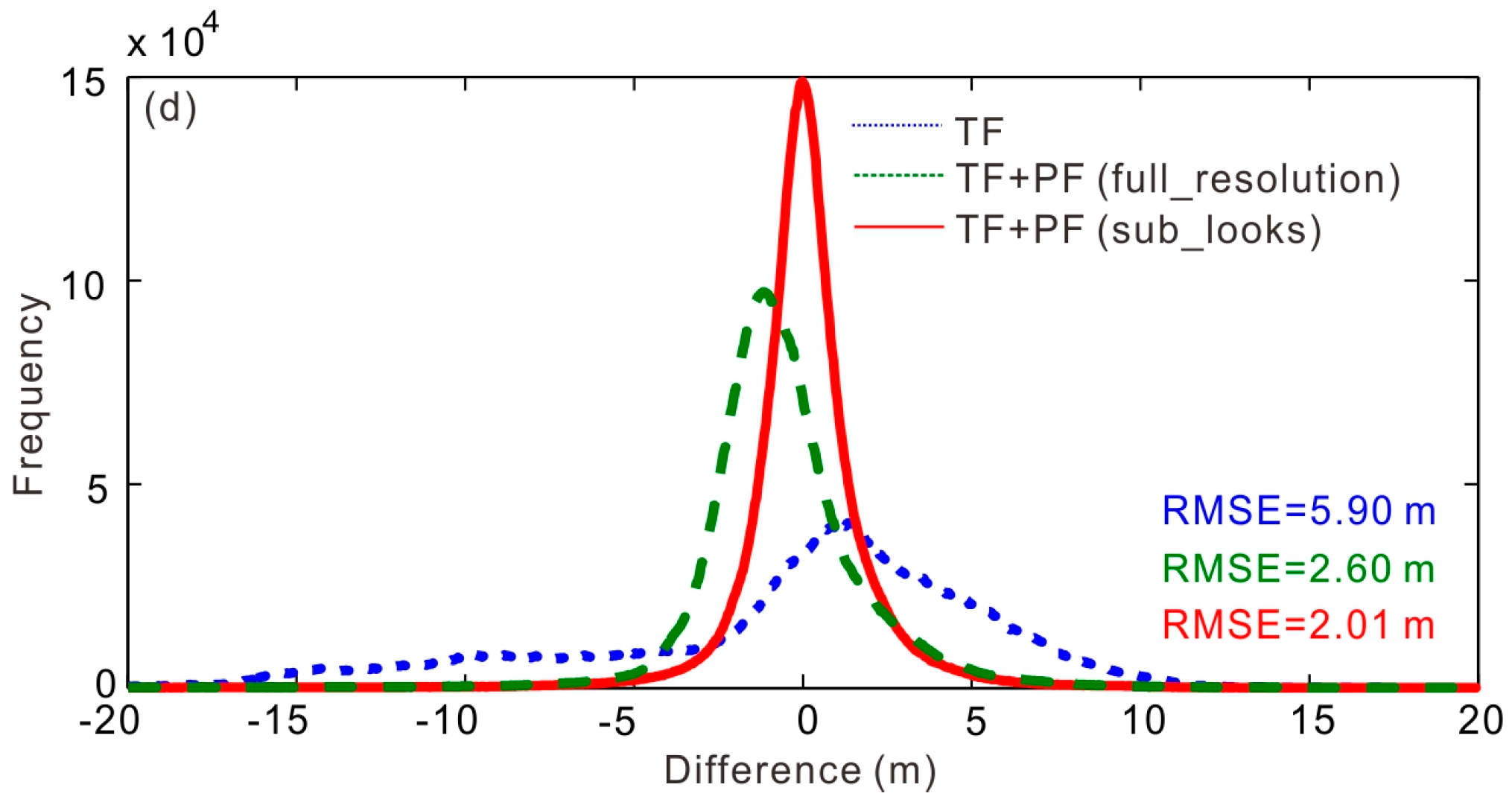
4.2. Influence of the RME on TF DEM Inversion

With the sub-look decomposition, sub-look interferograms characterized by different azimuth look angles were generated. One of the sub-look interferograms is displayed in Figure 7a (the flat-earth phase and the topography phase have been removed). It can be observed that there are some phase ramps caused by the RME along the azimuth direction, and it is difficult to distinguish the interferometric phase attributed to the forest height signal. The PF method was then used to extract the RME, as shown in Figure 7b. It can be observed that the RME is time-varying along the azimuth direction. Finally, the corrected interferogram was generated and is displayed in Figure 7c. The phase undulations have disappeared and the corrected interferogram seems to be dominated by topographic and forest height effects. This indicates that the PF method is able to remove the RME from the sub-look interferogram. To show the differences between the original and corrected interferograms directly, profiles of the above three interferograms at mid-range along the azimuth direction are presented in Figure 7d. As can be observed, the RME varies continuously and is characterized by long-wavelength components. After correction by the PF method, the interferometric phase does not present an obvious trend correlated with the azimuth direction.
Since the RME is time-varying along the azimuth direction, for every sub-look interferogram, they are distorted by different RMEs. In order to represent this, Figure 8a shows the difference map of two sub-look interferograms that have not had the RME corrected. It can be clearly observed that there are some phase undulations along the azimuth direction, which can be used to calculate the derivative of the RME. This prevents the accurate identification of phase centers for the sub-look interferograms. However, after calibration by the PF method, the difference map of the two sub-look interferograms is free from the influence of the RME, as shown in Figure 8b, and is mainly composed of the differences of the sub-look phase centers. Finally, a TF analysis of a resolution cell characterized by a 20-m forest height was conducted. Figure 8c shows the phase center height variation between sub-looks for the TF and TF+PF methods. It can be seen that, without the RME correction, the vertical distribution of the phase centers is significantly distorted. This indicates that RME correction is very important for TF analysis since the RME can lead to misunderstanding about the phase centers of the sub-look interferograms.
Finally, this study investigated the effect of the RME on the final DEM inversion. The ground phase map derived by the TF method is shown in Figure 9a. Phase undulations are obvious along the azimuth direction, and it is difficult to identify the phase components caused by the topography and forest height effects. This study also applied the PF method to correct the RME for the full-resolution interferogram. The extracted RME was then removed from the original slave image. Finally, the TF method was used to detect the ground phase, as shown in Figure 9b. When compared to Figure 9a, although most of the RME has been removed by this strategy, there are still some slight phase undulations along the azimuth direction. However, no phase undulation can be detected in the ground phase derived by the TF+PF method (sub-looks), as presented in Figure 9c. This suggests that even though correcting the RME for the full-resolution interferogram can reduce the impact of the RME on the result of the TF method, it is necessary to correct the RME by the PF method for every sub-look interferogram. In order to investigate the contribution of the RME to the DEM inversion, the TF, TF+PF (full resolution), and TF+PF (sub-looks) methods were used to extract the DEM. The errors of the three DEMs with respect to the LiDAR DEM are presented in Figure 9d. It can be noted that the RME can induce a large DEM error (RMSE = 5.90 m), while with the RME correction, the TF+PF (full resolution) and TF+PF (sub-looks) methods can provide more accurate DEM results, with RMSEs of 2.60 m and 2.01 m, respectively. In addition, this also confirms that it is reasonable to correct the RME for every sub-look interferogram.

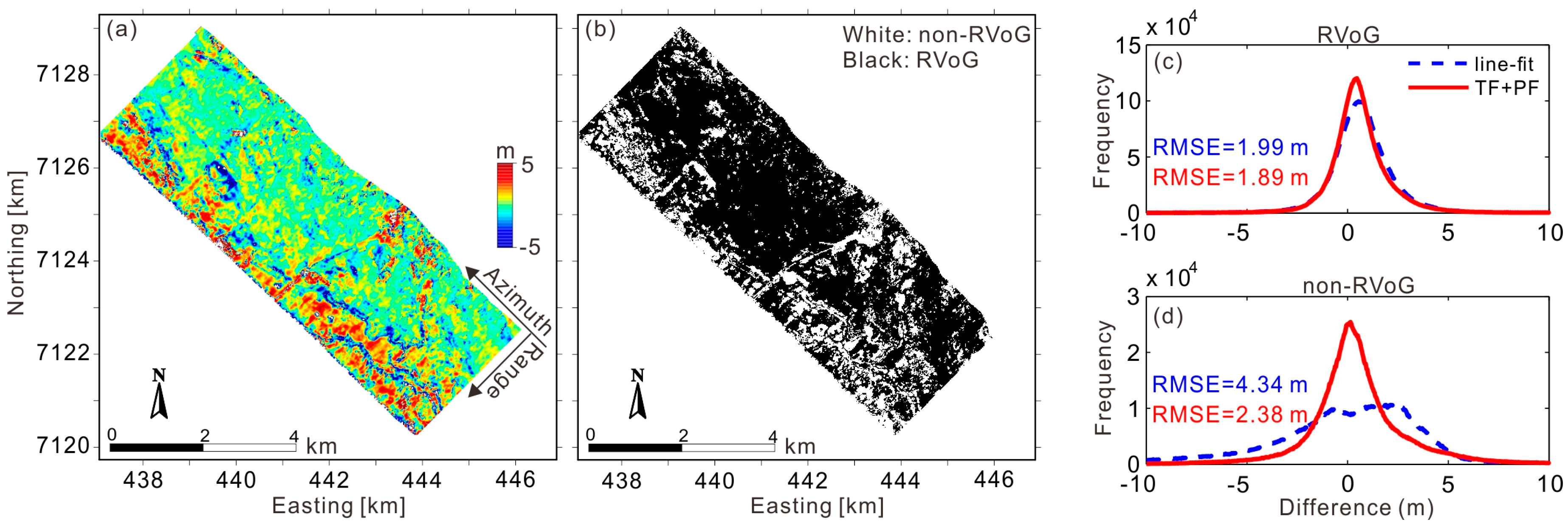
4.3. Influence of the RVoG Assumption on the DEM Inversion

Since the RVoG model plays an important role in PolInSAR techniques, the validity of the RVoG model should be checked before applying it to separate the ground contribution from the total PolInSAR signal. Several methods have been proposed for checking the validity [39,40]. Among them, the simple method proposed by Ballester-Berman et al. [40] is based on the difference between the topography values derived by the line-fit and Ω ( 1 , 2 ) T ( 2 , 1 ) methods. Similarly, the difference between the topography values estimated by the line-fit and TF+PF methods can also be used to test the RVoG assumption. The main idea is that, for a region where the RVoG assumption is fulfilled, the line-fit and TF+PF methods should provide approximate topography values since the line-fit method can extract reliable ground scattering contributions from the total PolInSAR signal. In contrast, if the RVoG assumption is not fulfilled, the topography values obtained by the two methods will be quite different since the ground interferometric phase is biased by the orientation effect. A critical problem with Ballester-Berman’s method is setting a proper threshold to describe the difference. To solve this problem, Ballester-Berman set the threshold as the average of the differences [38], which is not an adaptive threshold. As a result, this threshold may lead to some misunderstanding about the validity of the RVoG assumption. Therefore, in this study, the threshold was adaptively set as a function of the forest height, as shown in Figure 5c. According to previous research into forest height estimation and the magnitude error of the forest height, a realistic value for this threshold is 10–15% of the forest height [40]. Therefore, in this study, the threshold was set as 10% of the forest height. If the difference is lower than or equal to the threshold, the RVoG assumption is fulfilled. Otherwise, the region can be regarded as a non-RVoG zone. It should be noted that the forest height variation between 2006 and 2008 could lead to some underestimation of the threshold, resulting in some RVoG zones being regarded as non-RVoG zones. However, since the underestimation of the threshold is small, this cannot have a significant influence on the test of the RVoG assumption, and is not considered in this paper.
The difference map of the two DEMs is shown in Figure 10a. There are clear differences between both DEMs that are even more noticeable in the far range. This confirms the fact that it is necessary to set an adaptive threshold for the Ballester-Berman method. Finally, the result of the RVoG test is displayed in Figure 10b, where the non-RVoG zones are marked by white points. It can be observed that there are more non-RVoG zones in the far range with larger incidence angles. The reason for this is that the GVR decreases with the incidence angle [10,40]. Consequently, the line-fit method cannot give an accurate ground phase over the heterogeneous forest, as discussed in Section 2. This incidence-angle-dependent bias can be reduced by using multi-baseline or multi-angle PolInSAR data, considering the polarimetric conditions [15].
In order to investigate the differences in the DEMs derived by the line-fit and TF+PF methods in RVoG and non-RVoG zones, we generated histograms (Figure 10c,d) of the DEM errors. As Figure 10c shows, the two methods provide similar topography values in the RVoG zones, with RMSEs of 1.99 m and 1.89 m for the line-fit and TF+PF methods, respectively. However, in the non-RVoG zones, the RMSE (4.34 m) of the line-fit DEM is much higher than that of the TF+PF method (2.38 m). In addition, the DEM errors of the RVoG and non-RVoG zones for the line-fit method are quite different. However, this does not happen in the TF+PF result, which confirms that the TF+PF method is independent of the RVoG assumption and more suitable for DEM extraction in the P-band.

5. Discussion

This paper demonstrates that the TF+PF method can be used to estimate the ground scattering contribution from single-baseline PolInSAR data without depending on any assumption of the forest layer. In this procedure, the PF method is important since it can eliminate the effect of the RME on the interpretation of phase centers associated with different sub-looks. The performance of the PF method depends on the quality of the external DEM, which determines whether the RME can be detected through the differential interferometry. If the differential interferometric phase is dominated by the topographic error phase, and the RME can hardly be detected, in such a case, the PF model will be less sensitive to the RME. However, the existing works have shown that the global SRTM DEM can be used to simulate the ground phase in airborne differential interferometry, meeting the requirement of RME detection [27,30]. Furthermore, with a higher accuracy and higher resolution, the TanDEM-X DEM will also support more reliable differential interferometry. As a result, the performance of the PF method is not limited by the lack of a suitable external DEM. Moreover, it is possible to use the PF method to remove the RME for spaceborne interferometry. Compared with airborne platforms, spaceborne platforms are more stable. As a result, the corresponding RME is spatially smoother, which helps to prevent significant differences in the sub-look phase centers. However, this RME still needs to be removed since it can distort the interferogram and destroy the DEM quality. Compared with the linear or high-order plane models widely adopted in spaceborne interferometry, the PF method is more sensitive to the time-varying trend along the azimuth direction, which can help us to better process the RME. To remove the RME from the spaceborne interferometric phase, the order of Equation (9) should be adjusted to 1 or 2 since the vertical baselines are similar from the near range to the far range.
Apart from the TF+PF method, for the Krycklan test site, the tomographic SAR method has also been applied to extract the underlying DEM with six L-band SAR images [41]. A DEM with an RMSE of about 2.0 m was achieved, which is in agreement with the DEM derived by the TF+PF method. This confirms that the TF method is able to detect the ground scattering contributions for this test site. However, this may not be the case over dense forest, such as tropical forest, because the SAR signals undergo significant attenuation, and it is difficult for the TF method to detect pure ground scattering contributions. Whether or not the TF method will still perform well over dense forest requires further study. Moreover, the ground scattering contributions are related to the terrain slope [15]. It is therefore worth specifying the relationship between the DEM error and the terrain slope, which could help us to better understand the application scope of the TF method.
The results obtained in this paper have to be carefully assessed in the context of the spaceborne BIOMASS mission. In the case of the BIOMASS mission, the limited pulse bandwidth of 6 MHz [42,43] can induce a low resolution (12.5 m × 25 m [43]) and a narrow observation angle interval. Compared with an airborne high-resolution cell, a low-resolution cell contains more scattering targets, which makes it more difficult for the SAR sensor to “see” the ground directly, due to the mixed scattering contributions. Furthermore, the narrow observation angle interval reduces the possibility of detecting a more pure ground scattering contribution. As a result, the DEM derived by the TF method can be affected by the forest height signal. However, considering the low resolution, this elevation bias may be acceptable. In addition to the narrow bandwidth effects, other effects also need to be taken into account. These include the temporal decorrelation effects, ionospheric effects, and atmospheric effects. Although the impact of temporal decorrelation can be negligible for the topographic phase when the revisit time is less than four days [43], it is still necessary to assess the influence of coherence loss on the interferometric phase, combining the information acquired by the TropiScat campaign [44]. The ionospheric effects can be mitigated by computing the Faraday rotation [45] or performing phase gradient autofocus [46]. Consequently, ionospheric effects do not result in significant error in DEM estimation. However, differing from the ionospheric effects, atmospheric effects cannot be easily removed without the help of external water vapor data, and atmospheric effects can severely distort the interferometric phase and cause unacceptable DEM error. Therefore, it is necessary to expand the TF+PF method to the framework of time-series InSAR, allowing the atmospheric effects to be reduced through temporal-spatial analysis [31]. Nonetheless, the TF analysis method may be a good candidate for the future BIOMASS mission to extract the underlying DEM in forest areas [42].

6. Conclusions

In this paper, a method based on a TF approach combined with a polynomial fitting method to correct the RME has been proposed for underlying topography estimation in forest areas. With this method, the ground scattering contribution can be directly separated from the total PolInSAR signal without resorting to any physical model of the forest. The proposed method is suitable for P-band SAR data, which has a significant penetration depth and sufficient observation angle interval in the azimuth direction.
The Krycklan catchment test site was selected to test the performance of the TF+PF method for DEM inversion. The TF+PF-derived DEM has an RMSE of 2.01 m, which is more accurate than that derived by the line-fit method (with an RMSE = 2.75 m). Moreover, it is known that the RME can distort the result of the TF method, and it is necessary to correct the RME for every sub-look interferogram. Finally, a quantitative analysis of DEM inversion was conducted over the RVoG and non-RVoG zones. The results also show that the accuracy of the TF+PF DEM is independent of the RVoG assumption.

Acknowledgments

This work was supported by the National Natural Science Foundation of China (No. 41531068, 41371335, 41671356, and 41274010) and the Hunan Provincial Innovation Foundation for Postgraduate (No. 150140004). The paper was also supported by the PA-SB ESA EO Project Campaign.

Author Contributions

Haiqiang Fu conceived of the idea, designed the experiments, and wrote and revised the paper; Jianjun Zhu performed the PolInSAR experiments and revised the paper; Changcheng Wang analyzed the experimental results; Huiqiang Wang and Rong Zhao revised the paper and drew some of the figures.

Conflicts of Interest

The authors declare no conflict of interest.

References

  1. Sun, Q.; Zhang, L.; Ding, X.L.; Hu, J.; Li, Z.W.; Zhu, J.J. Slope deformation prior to Zhouqu, China landslide from InSAR time series analysis. Remote Sens. Environ. 2015. [Google Scholar] [CrossRef]
  2. Baugh, C.A.; Bates, P.D.; Schumann, G.; Trigg, M.A. SRTM vegetation removal and hydrodynamic modeling accuracy. Water Resour. Res. 2013, 49, 5276–5289. [Google Scholar] [CrossRef]
  3. Farr, T.G.; Rosen, P.A.; Caro, E.; Crippen, R.; Duren, R.; Hensley, S.; Kobrick, M.; Paller, M.; Rodriguez, E.; Roth, L.; et al. The shuttle radar topography mission. Rev. Geophys. 2007. [Google Scholar] [CrossRef]
  4. Huber, M.; Gruber, A.; Wendleder, A.; Wessel, B.; Roth, A.; Schmitt, A. The global Tandem-X DEM: Production status and first validation results. In Proceedings of the International Society for Photogrammetry and Remote Sensing, Melbourne, Australia, 25 August–1 September 2012. [Google Scholar]
  5. Balzter, H.; Baade, J.; Rogers, K. Validation of the TanDEM-X intermediate digital elevation model with airborne LiDAR and differential GNSS in Kruger National Park. IEEE Geosci. Remote Sens. Lett. 2016, 13, 277–281. [Google Scholar] [CrossRef]
  6. Cloude, S.R.; Papathanassiou, K.P. Polarimetric SAR interferometry. IEEE Trans. Geosci. Remote Sens. 1998, 36, 1551–1565. [Google Scholar] [CrossRef]
  7. Papathanassiou, K.P.; Cloude, S.R. Single-baseline polarimetric SAR interferometry. IEEE Trans. Geosci. Remote Sens. 2001, 39, 2352–2363. [Google Scholar] [CrossRef]
  8. Cloude, S.R.; Papathanassiou, K.P. Three-stage inversion process for polarimetric SAR interferometry. IEEE Proc. Radar Sonar Navig. 2003, 150, 125–134. [Google Scholar] [CrossRef]
  9. Ballester-Berman, J.D.; Lopez-Sanchez, J.M. Applying the Freeman–Durden decomposition concept to polarimetric SAR interferometry. IEEE Trans. Geosci. Remote Sens. 2010, 48, 466–479. [Google Scholar] [CrossRef]
  10. Lopez-Martinez, C.; Papathanassiou, K.P. Cancellation of scattering mechanisms in PolInSAR: Application to underlying topography estimation. IEEE Trans. Geosci. Remote Sens. 2013, 51, 953–965. [Google Scholar] [CrossRef]
  11. Fu, H.; Wang, C.; Zhu, J.; Xie, Q.; Zhao, R. Inversion of forest height from PolInSAR using complex least squares adjustment method. Sci. China Earth Sci. 2015, 58, 1018–1031. [Google Scholar] [CrossRef]
  12. Fu, H.; Wang, C.; Zhu, J.; Xie, Q.; Zhang, B. Estimation of pine forest height and underlying DEM using multi-baseline P-band PolInSAR data. Remote Sens. 2016, 8, 820. [Google Scholar] [CrossRef]
  13. Treuhaft, R.N.; Madsen, S.N.; Moghaddam, M.; Van Zyl, J.J. Vegetation characteristics and underlying topography from interferometric data. Radio Sci. 1996, 31, 1449–1495. [Google Scholar] [CrossRef]
  14. Treuhaft, R.N.; Siqueira, P.R. Vertical structure of vegetated land surfaces from interferometric and polarimetric data. Radio Sci. 2000, 35, 141–177. [Google Scholar] [CrossRef]
  15. Hajnsek, I.; Kugler, F.; Lee, S.K.; Papathanassiou, K.P. Tropical-forest-parameter estimation by means of Pol-InSAR: The INDREX-II campaign. IEEE Trans. Geosci. Remote Sens. 2009, 47, 481–492. [Google Scholar] [CrossRef]
  16. Kugler, F.; Schulze, D.; Hajnsek, I.; Pretzsch, H.; Papathanassiou, K.P. TanDEM-X Pol-InSAR performance for forest height estimation. IEEE Trans. Geosci. Remote Sens. 2014, 52, 6404–6422. [Google Scholar] [CrossRef]
  17. Lee, S.K.; Kugler, F.; Papathanassiou, K.P.; Hajnsek, I. Quantification of temporal decorrelation effects at L-band for polarimetric SAR interferometry applications. IEEE J. Sel. Top. Appl. Earth Obs. Remote Sens. 2013, 6, 1351–1367. [Google Scholar] [CrossRef]
  18. Garestier, F.; Le Toan, T. Forest modeling for height inversion using single baseline InSAR/Pol-InSAR data. IEEE Trans. Geosci. Remote Sens. 2010, 48, 1528–1539. [Google Scholar] [CrossRef]
  19. Treuhaft, R.N.; Cloude, S.R. The structure of oriented vegetation from polarimetric interferometry. IEEE Trans. Geosci. Remote Sens. 1999, 37, 2620–2624. [Google Scholar] [CrossRef]
  20. Cloude, S.R. Polarisation: Applications in Remote Sensing; Oxford University Press: New York, NY, USA, 2009. [Google Scholar]
  21. Lopez-Sanchez, J.M.; Ballester-Berman, J.D.; Marquez-Moreno, Y. Model limitations and parameter-estimation methods for agricultural applications of polarimetric SAR interferometry. IEEE Trans. Geosci. Remote Sens. 2007, 45, 3481–3493. [Google Scholar] [CrossRef]
  22. Lopez-Sanchez, J.M.; Hajnsek, I.; Ballester-Berman, J.D. First demonstration of agriculture height retrieval with PolInSAR airborne data. IEEE Geosci. Remote Sens. Lett. 2012, 9, 242–246. [Google Scholar] [CrossRef]
  23. Garestier, F.; Dubois-Fernandez, P.C.; Papathanassiou, K.P. Pine forest height inversion using single-pass X-band PolInSAR data. IEEE Trans. Geosci. Remote Sens. 2008, 46, 56–68. [Google Scholar] [CrossRef]
  24. Garestier, F.; Dubois-Fernandez, P.; Champion, I. Forest height inversion using high resolution P-band Pol-InSAR data. IEEE Trans. Geosci. Remote Sens. 2008, 46, 3544–3559. [Google Scholar] [CrossRef]
  25. Ferro-Famil, L.; Reigber, A.; Pottier, E.; Boerner, W.M. Scene characterization using subaperture polarimetric SAR data. IEEE Trans. Geosci. Remote Sens. 2003, 41, 2264–2276. [Google Scholar] [CrossRef]
  26. Reigber, A.; Prats, P.; Mallorqui, J.J. Refined estimation of time-varying baseline errors in airborne SAR interferometry. IEEE Geosci. Remote Sens. Lett. 2006, 3, 145–149. [Google Scholar] [CrossRef]
  27. De Macedo, K.A.C.; Scheiber, R.; Moreira, A. An autofocus approach for residual motion errors with application to airborne repeat-pass SAR interferometry. IEEE Trans. Geosci. Remote Sens. 2008, 46, 3151–3162. [Google Scholar] [CrossRef]
  28. DLR Microwaves and Radar Institute; Swedish Defense Research Agency; Politecnico di Milano POLIMI. BIOSAR 2008: Data Acquisition and Processing Report. 2008. Available online: https://earth.esa.int/c/document_library/get_file?folderId=21020&name=DLFE-903.pdf (accessed on 17 February 2017).
  29. Flynn, T.; Tabb, M.; Carande, R. Coherence region shape extraction for vegetation parameter estimation in polarimetric SAR interferometry. In Proceedings of the 2002 IEEE International Geoscience and Remote Sensing Symposium, Toronto, ON, Canada, 24–28 June 2002; pp. 2596–2598. [Google Scholar]
  30. Bianco, V.; Pardini, M.; Papathanassiou, K.; Iodice, A. Phase calibration of multibaseline SAR data stacks: A minimum entropy approach. In Proceedings of the 2012 IEEE International Geoscience and Remote Sensing Symposium, Munich, Germany, 22–27 July 2012; pp. 5198–5201. [Google Scholar]
  31. Prats, P.; Reigber, A.; Mallorqui, J.J.; Scheiber, R.; Moreira, A. Estimation of the temporal evolution of the deformation using airborne differential SAR interferometry. IEEE Trans. Geosci. Remote Sens. 2008, 46, 1065–1078. [Google Scholar] [CrossRef]
  32. De Macedo, K.A.C.; Wimmer, C.; Barreto, T.L.M.; Lübeck, D.; Moreira, J.R.; Rabaco, L.M.L.; de Oliveira, W.J. Long-term airborne DInSAR measurements at X and P-bands: A case study on the application of surveying geohazard threats to pipelines. IEEE J. Sel. Top. Appl. Earth Obs. Remote Sens. 2012, 5, 990–1005. [Google Scholar] [CrossRef]
  33. Small, D. Generation of Digital Elevation Models through Spaceborne SAR Interferometry. Ph.D. Thesis, University of Zurich, Zürich, Switzerland, 1998. [Google Scholar]
  34. Xu, B.; Li, Z.; Wang, Q.; Jiang, M.; Zhu, J.; Ding, X. A refined strategy for removing composite errors of SAR interferogram. IEEE Geosci. Remote Sens. Lett. 2014, 11, 143–147. [Google Scholar] [CrossRef]
  35. Shirzaei, M. A wavelet-based multitemporal DInSAR algorithm for monitoring ground surface motion. IEEE Geosci. Remote Sens. Lett. 2013, 3, 456–460. [Google Scholar] [CrossRef]
  36. Tao, K.; Zhu, J. A hybrid indicator for determining the best decomposition scale of wavelet denoising. Acta Geod. Cartogr. Sin. 2012, 41, 749–755. [Google Scholar]
  37. Li, Z.; Ding, X.; Huang, C.; Zhu, J.; Chen, Y. Improved filtering parameter determination for the Goldstein radar interferogram filter. ISPRS J. Photogramm. 2008, 63, 621–634. [Google Scholar] [CrossRef]
  38. Chen, C.; Zebker, H. Two-dimensional phase unwrapping with use of statistical models for cost function in nonlinear optimization. J. Opt. Soc. Am. A 2001, 18, 338–351. [Google Scholar] [CrossRef]
  39. Lopez-Martinez, C.; Alonso-Gonzalez, A. Assessment and estimation of the RVoG model in polarimetric SAR interferometry. IEEE Trans. Geosci. Remote Sens. 2014, 52, 3091–3106. [Google Scholar] [CrossRef]
  40. Ballester-Berman, J.D.; Vicente-Guijalba, F.; Lopez-Sanchez, J.M. A simple RVoG test for PolInSAR data. IEEE J. Sel. Top. Appl. Earth Obs. Remote Sens. 2015, 8, 1028–1040. [Google Scholar] [CrossRef]
  41. Pardini, M.; Papathanassiou, K. Sub-canopy topography estimation: Experiments with multibaseline SAR data at L-band. In Proceedings of the 2012 IEEE International Geoscience and Remote Sensing Symposium, Munich, Germany, 22–27 July 2012; pp. 4954–4957. [Google Scholar]
  42. Le Toan, T.; Quegan, S.; Davidson, M.W.J.; Balzter, H.; Paillou, P.; Papathanassiou, K.P.; Plummer, S.; Rocca, F.; Saatchi, S.; Shugart, H.; et al. The BIOMASS mission: Mapping global forest biomass to better understand the terrestrial carbon cycle. Remote Sens. Environ. 2011, 115, 2850–2860. [Google Scholar] [CrossRef]
  43. Ho Tong Minh, D.; Tebaldini, S.; Rocca, F.; Le Toan, T.; Villard, L.; Dubois-Fernandez, P.C. Capabilities of BIOMASS tomography for investigating tropical forests. IEEE Trans. Geosci. Remote Sens. 2015, 53, 965–975. [Google Scholar] [CrossRef]
  44. Hamadi, A.; Borderies, P.; Albinet, C.; Koleck, T.; Villard, L.; Ho Tong Minh, D.; Le Toan, T.; Burban, B. Temporal coherence of tropical forests at P-band: Dry and rainy seasons. IEEE Geosci. Remote Sens. Lett. 2015, 12, 557–561. [Google Scholar] [CrossRef]
  45. Rosen, P.; Lavalle, M.; Pi, X.; Gurrola, E. Techniques and tools for estimating ionospheric effects in interferometric and polarimetric SAR data. In Proceedings of the 2011 IEEE International Geoscience and Remote Sensing Symposium, Vancouver, BC, Canada, 24–29 July 2011; pp. 1501–1504. [Google Scholar]
  46. Li, Z.; Quegan, S.; Chen, J.; Rogers, N.C. Performance analysis of phase gradient autofocus for compensating ionospheric phase scintillation in BIOMASS P-band SAR data. IEEE Geosci. Remote Sens. Lett. 2015, 12, 1367–1371. [Google Scholar]
Figure 1. Geometrical interpretation of (a) random-volume-over-ground (RVoG) and (b) oriented-volume-over-ground (OVoG).
Remotesensing 09 00363 g001
Figure 2. Variation of ground height error derived by the line-fit model with (a) the extinction; (b) the ground-to-volume ratio (GVR); and (c) the vertical wavenumber in the OVoG model.
Remotesensing 09 00363 g002
Figure 3. (a) Frequency spectral filtering effect on the azimuth observation angle [24]; (b) Subaperture processing with different azimuth observation angles.
Remotesensing 09 00363 g003
Figure 4. The flowchart of digital elevation model (DEM) inversion based on the time-frequency (TF) method. (a) Sub-look interferogram generation; (b) RME removal for every sub-look interferogram; (c) DEM generation.
Remotesensing 09 00363 g004
Figure 5. (a) P-band synthetic aperture radar (SAR) image on the Pauli basis (R: HH − VV; G: HV; B: HH + VV); (b) LiDAR-derived DEM; (c) LiDAR-derived forest height.
Remotesensing 09 00363 g005
Figure 6. The DEM results. (a) Line-fit derived DEM; (b) TF+ polynomial fitting (PF)–derived DEM; (c) Histograms of the DEM difference; (d) DEM error for the line-fit method; (e) DEM error for the TF+PF method; (f) Histograms of the DEM errors derived by the line-fit and TF+PF methods.
Remotesensing 09 00363 g006
Figure 7. Influence of the RME on the sub-look differential interferogram (the flat-earth phase and topography phase have been removed). (a) One original sub-look differential interferogram; (b) RME extracted with the PF method; (c) The differential interferogram corrected by the TF method; (d) Profiles of the above three differential interferograms at mid-range along the azimuth direction.
Remotesensing 09 00363 g007
Figure 8. Influence of the RME on the TF analysis. (a) Difference map of two sub-look interferograms generated by the TF method; (b) Difference map of two sub-look interferograms generated by the TF+PF method; (c) Phase center height variations between sub-looks for the TF and TF+PF methods.
Remotesensing 09 00363 g008
Figure 9. Influence of the RME on the DEM inversion. Ground phases (the flat-earth phase and topography phase have been removed) derived by (a) the TF method; (b) the TF+PF method (corrected full-resolution interferogram); and (c) the TF+PF method (corrected sub-look interferogram); (d) Histograms of the DEM errors derived by the TF, TF+PF (full resolution), and TF+PF (sub-looks) methods.
Remotesensing 09 00363 g009aRemotesensing 09 00363 g009b
Figure 10. Test of the RVoG assumption. (a) DEM difference map; (b) Binary map, with white for non-RVoG and black for RVoG; (c) Histograms of the DEM errors in the RVoG region; (d) Histograms of the DEM errors in the non-RVoG region.
Remotesensing 09 00363 g010
Table 1. Parameters of the three simulation experiments.
Ground Height (m)Vegetation Height (m)Extinction (dB/m)GVRkz
100–30t × (1:0.5:0), 0 ≤ t ≤ 3(0:0.5:1)0.15
2(1:0.5:0)t × (0:0.5:1), 0 ≤ t ≤ 30.15
3(1:0.5:0)(0:0.5:1)0.01–0.2
Table 2. Parameters of the two interferometric pairs.
Test SiteRange × Azimuth kz RangeIncidence AngleTemporal Baseline
Krycklan1.5 × 2.0 m0.055–0.24525°–52°70 min

