
Spectral-Spatial Response for Hyperspectral Image Classification


Abstract
:
1. Introduction
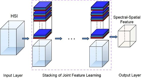
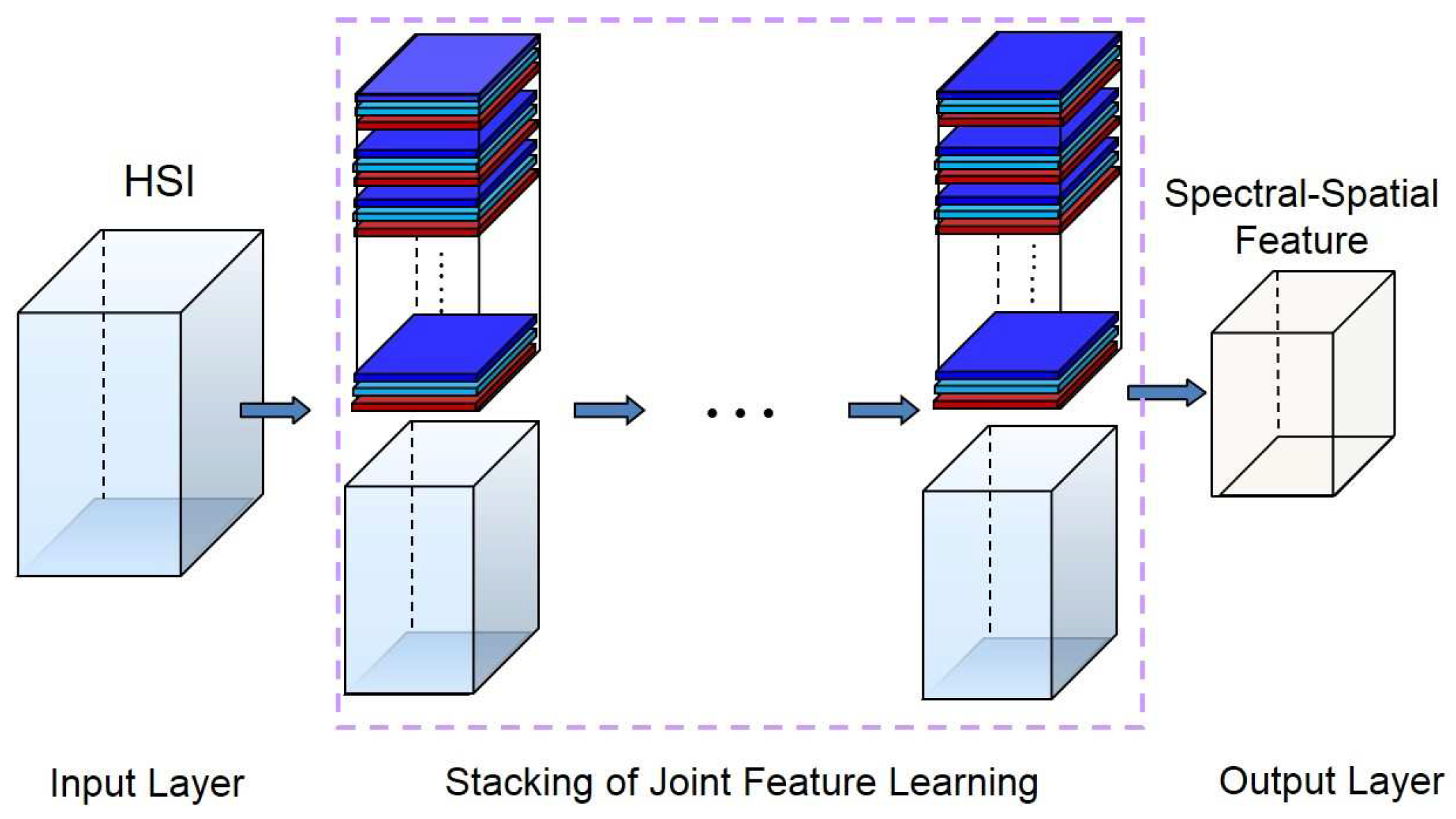
- SSR provides a new way to simultaneously exploit discriminative spectral and spatial information in a deep hierarchical fashion. The stacking of joint spectral-spatial feature learning units can produce intrinsic features of HSIs.
- SSR is a unified framework of designing new joint spectral-spatial feature learning methods for HSI classification. Several existing spectral-spatial-based methods are its special cases.
- As an implementation example of SSR, SLN is further introduced for HSI classification with a small number of training samples. It is easy to implement and has low sample complexity.
2. Spectral-Spatial Response
2.1. Definition of Spectral-Spatial Response
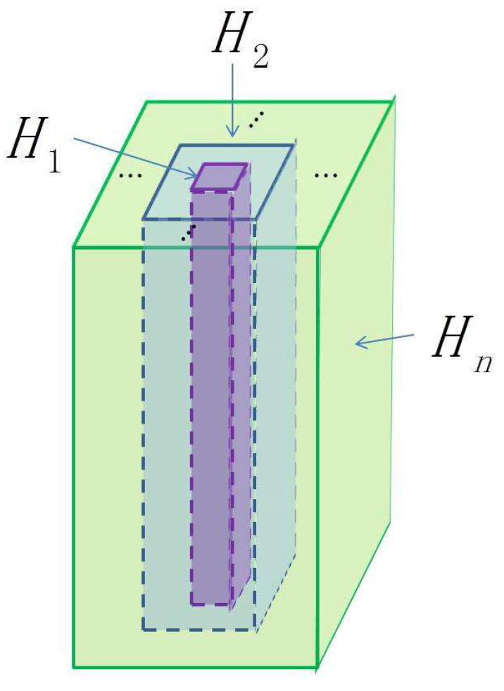
- A finite number of nested cubes to define the hierarchical architecture (see Figure 1). The SSRs on different layers can be learned from different cubes. The sizes of cubes determine the sizes of neighborhoods in the original HSI.
- A set of templates (or filters) that extract the spectral and spatial features. These templates can be learned from the training samples or the cubes centered at positions of the training samples.
- (1)
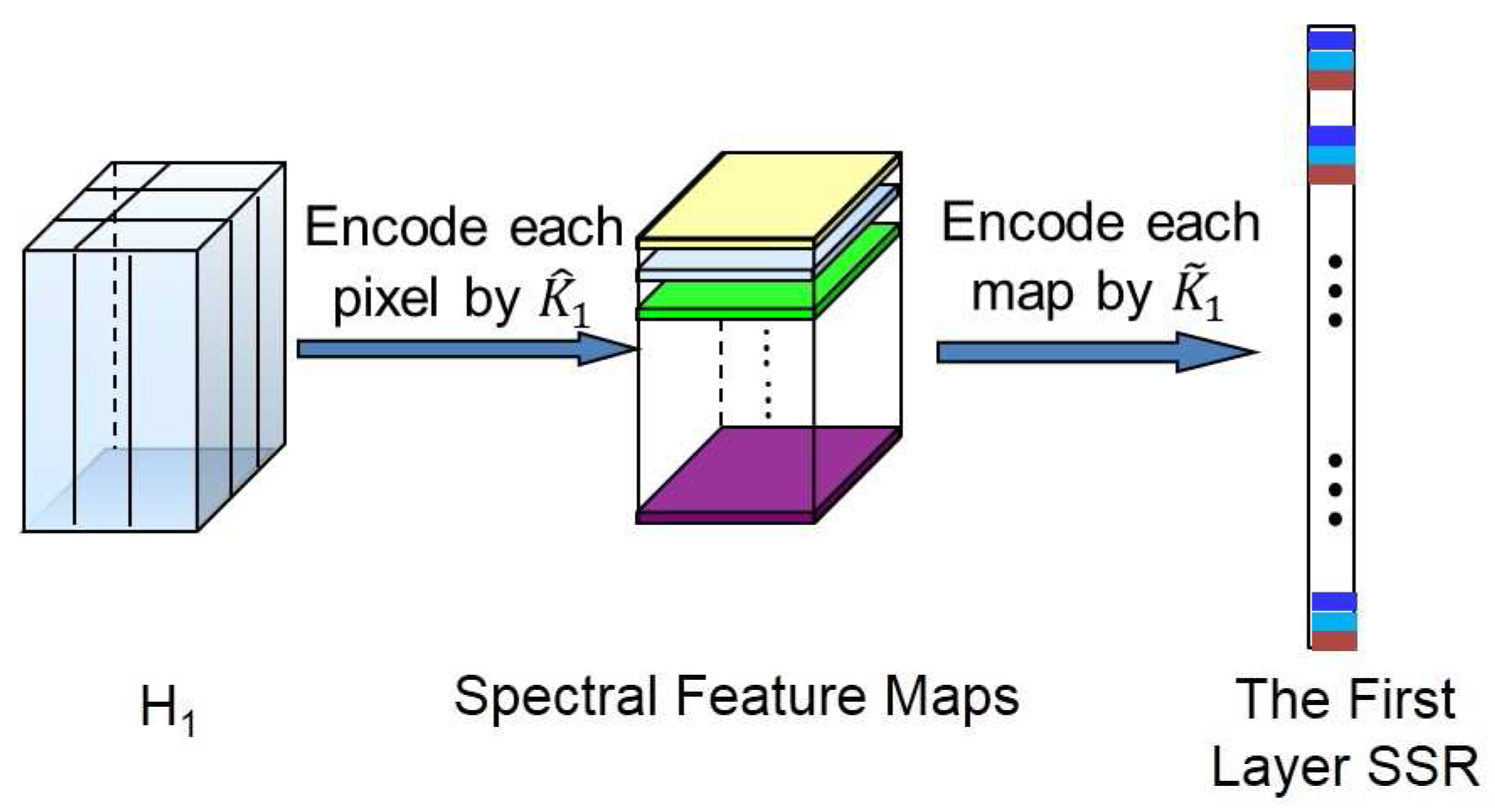
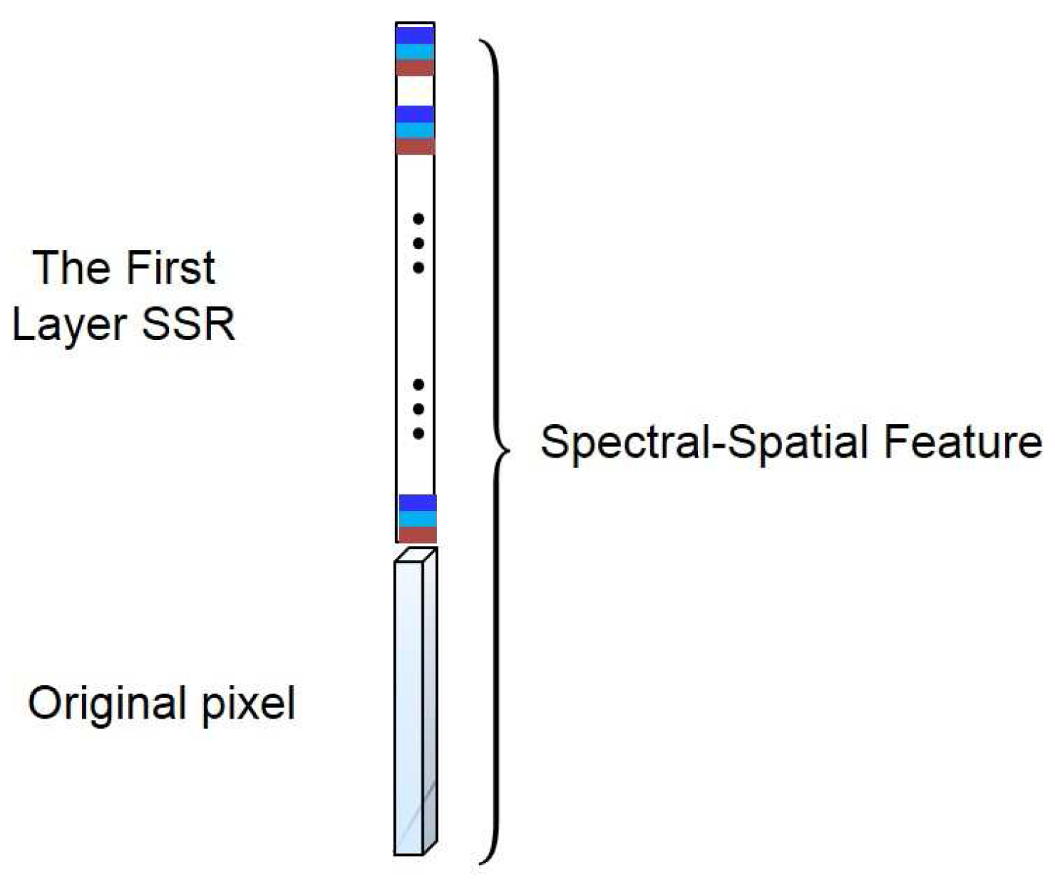
- The first layer SSR:The computation procedure of the first layer SSR is shown in Figure 2. Let be the central pixel of , then the spectral-spatial feature of can be jointly learned as follows.First, the spectral features can be learned from each pixel. The reproducing kernel, denoted by , can be used to learn the spectral features, where is a pixel in and is the l-th spectral template in . The reproducing kernel can produce the spectral features by encoding the pixel by a set of learned templates. For example, one could choose the simple linear kernel, namely:The spectral templates are spectral feature extractors learned from training pixels. This operation intends to reduce the spectral redundancy. In this way, pixel can be transformed into a -dimensional feature vector,where is the cardinality of the and . Similarly, pixels in (the pixel and its neighborhoods) can be transformed to a new cube in , where is the size of the neighborhoods. In this cube, there are matrices of size . Here, these matrices are called the first layer spectral feature maps, denoted by . Note that at this stage, we can move pixel by pixel.Second, we learn the spatial features based on the outputs of the previous stage . In this stage, our objective is to incorporate spatial contextual information within the neighbor into the processing pixel. We have:where:and spatial template can be learned from the first layer spectral feature maps of the training samples. In this way, for each , we can obtain a new feature vector:where is called the first layer SSR of . This operation can be considered as the “convolution” in the conventional deep learning model. In this way, the spatial information of the local region can be learned. Consequently, the first layer SSR is obtained by jointly exploiting both spectral and spatial information of the HSI.Finally, we concatenate and into a new spectral-spatial feature vector (see Figure 3). It can provide more spectral information. In this way, the spectral feature can be enhanced, and the oversmooth problem can be overcome. We processed all of the pixels in , then a new feature cube denoted by can be obtained. Note that each feature vector in is learned from a cube with size of in the original HSI.
- (2)
- The second layer SSR:Similarly, we can define the second layer SSR on a region corresponding to in the original image . In this case, two template sets are denoted by and , respectively. For each , we have:where:can be regarded as the pooling operation over all spectral bands. The outputs of this operation on all positions are called the second layer spectral feature maps denoted by . Then, these maps can be convoluted by the learned templates (or filters) (). For the position , we have:Consequently, the second layer SSR on position can be defined by:where can be learned from all feature maps of training samples. Similarly, the final output is obtained by concatenating and into a new spectral-spatial feature.
- (3)
- Extend to n layers:The output of the previous step is a new feature cube. Similarly, the definition given above can be easily generalized to an n layer architecture defined by sub-cubes .
- The proposed framework shares similarities with deep learning models. If kernel functions and jointly learn spectral-spatial features on the first layer, then the iterated mapping in Equation (10) demonstrates the multilayer feature learning in the deep model. Consequently, with the increase of the depth, the receptive field becomes larger and larger. In this way, the hierarchical architecture could propagate local information to a broader region. Thus, this framework can learn spectral-spatial features of the HSI with multiple levels of abstractions.
- The proposed framework is designed for HSI classification. This shows that and can learn spectral and spatial features jointly. They are not considered in the conventional deep learning models, which are very popular in the computer vision community. These kernel functions can be viewed as inducing a nonlinear mapping from inputs to feature vectors. can learn spectral features and overcome the high-dimension problem. Additionally, can learn spatial features and decrease the intraclass variations. Consequently, the proposed SSR is suitable for the nature of the HSIs.
- An HSI usually contains homogeneous regions. Consequently, we assume that each pixel in an HSI will likely share similar spectral characteristics or have the same class membership as its neighboring pixels. This is the reason why the spatial information can be used in the proposed framework SSR.
- In SSR, the template plays an important role, and it could be a filter or an atom of the dictionary. Consequently, constructing the template sets is an interesting problem to be further investigated.
- Stacking joint spectral-spatial feature learning leads to a deep architecture. Different feature learning methods (linear and nonlinear) can be embedded into the proposed SSR. The flexibility offers the possibility to systematically and structurally incorporate prior knowledge; for example, MFA can be used to learn discriminative features.
2.2. Special Scenarios
2.2.1. PCA+Gabor
2.2.2. Edge-Preserving Filtering
3. Subspace Learning-Based Networks
- (1)
- PreprocessingThe image preprocessing is to normalize the data values into by:where , and is the m-th band of pixel . The normalized HSI is denoted as .
- (2)
- Joint spectral-spatial feature learning:First, the discriminative spectral features are desired for classification. Consequently, the label information of the training samples can be used. In SLN, a supervised subspace learning method, MFA [62], is used to construct . MFA aims at searching for the projection directions on which the marginal sample pairs of different classes are far away from each other while requiring data points of the same class to be close to each other [63]. Here, the projection directions of MFA are taken as the templates in . Assume that there are templates and is the template set. The spectral templates are the eigenvectors corresponding to a number of the largest eigenvalues of:where is the normalized training set, is the Laplacian matrix and is the constraint matrix (refer to [62]). Once the templates are given, the normalized HSI can be projected to the templates pixel by pixel. As described in Section 2, each template produces a feature map. In this way, we can obtain spectral feature maps.Second, spatial information within the neighbor is expected to be incorporated into the processing pixel. In SLN, PCA as a linear autoencoder has been used to construct . In this way, the template learning method is simple and fast. The templates in can be learned as follows.We crop image patches centered at each training sample in the i-th spectral feature map. Because there are N training samples, we can collect N patches from each map. These cropped patches are vectorized and form a matrix . Matrix is then obtained after removing mean values. The construction of the template set is an optimization problem:where is the spatial template; that is, to find the principal eigenvectors of [64]. The patches cropped from each band of the training samples can be encoded by the templates. In this way, a feature cube can be obtained, where the number of its feature maps is . After that, we concatenate the obtained feature cube and normalized HSI into a new feature cube, where the height of the new feature cube is . Similarly, higher layer features can be obtained by extending this architecture to n. Consequently, SLN can extract deep hierarchical features.
- (3)
- Classification based on KELM:After L alternations of the joint spectral-spatial feature learning processes, SLN obtains spectral-spatial features that are then classified by the KELM classifier [15,17,65].Let the features of training samples be (), where and indicate classes and:The output of the KELM classifier is:where is the feature of the test sample, and K is the kernel function (this paper uses the Radial Basis Function (RBF) kernel). Finally, the class of the test sample is determined by the index of the output node with the highest output value [65].
| Algorithm 1 SLN: training procedure. |
|
| Algorithm 2 SLN: test procedure |
|
- As one implementation of SSR, SLN is a deep learning method. Similarly, other hierarchical methods can be obtained when applying different kinds of templates and kernels in SSR.
- The templates in SLN are learned by MFA and PCA, which are simple and have better performance in feature learning. Consequently, SLN is a simple and efficient method to jointly learn the spectral-spatial features of HSIs.
4. Experimental Results and Discussions
4.1. Datasets and Experimental Setups
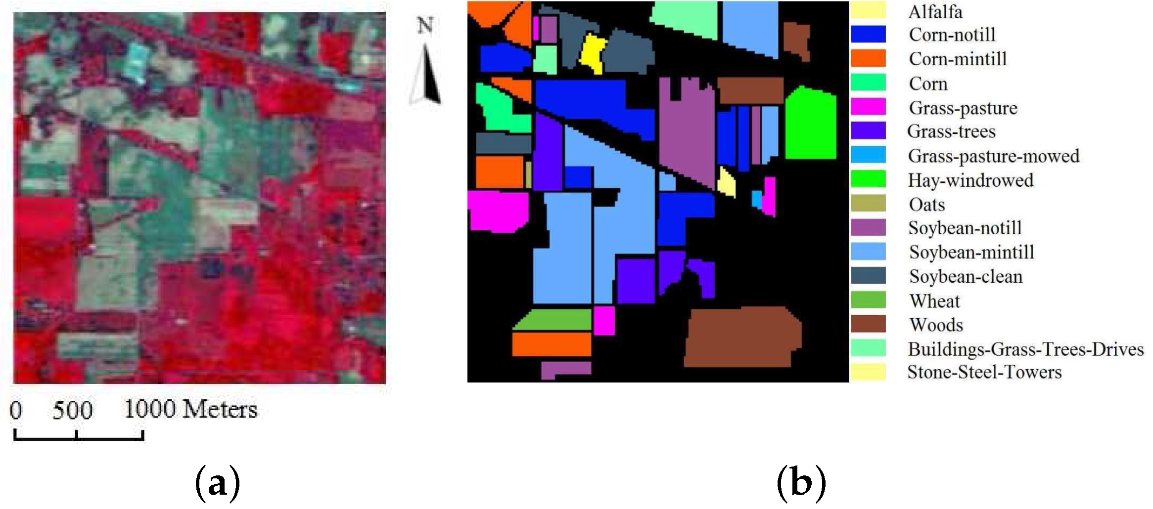
- The Indian Pines dataset was acquired by the AVIRIS sensor over the Indian Pines test site in 1992 [67]. The image scene contains pixels and 220 spectral bands. The ground truth available is designated into 16 classes. In the experiments, the number of bands has been reduced to 200 due to atmospheric effects. This scene is challenging because of the significant presence of mixed pixels and the unbalanced number of available labeled pixels in each class [35]. A three-band false color image and the ground-truth image are shown in Figure 5.
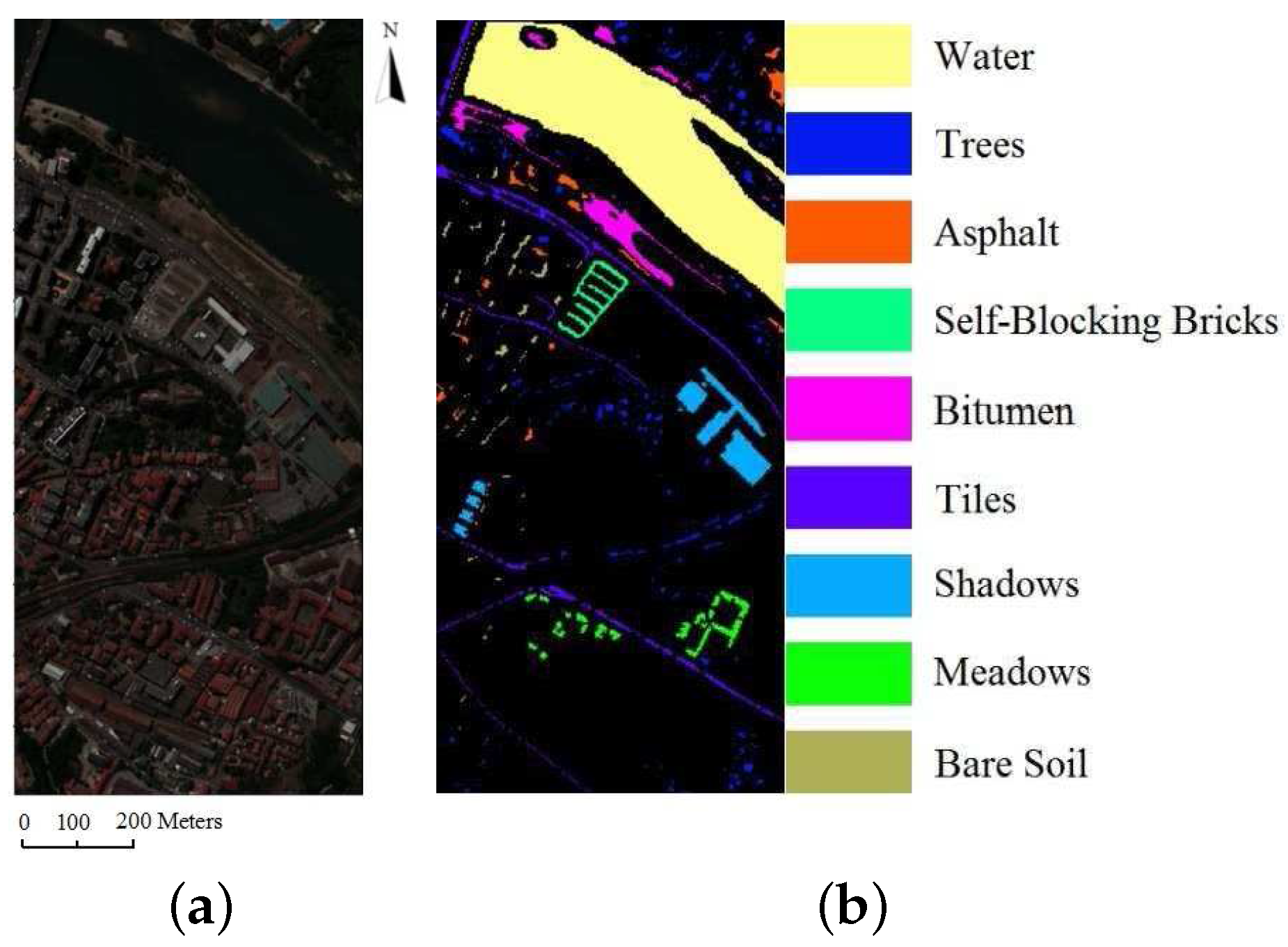
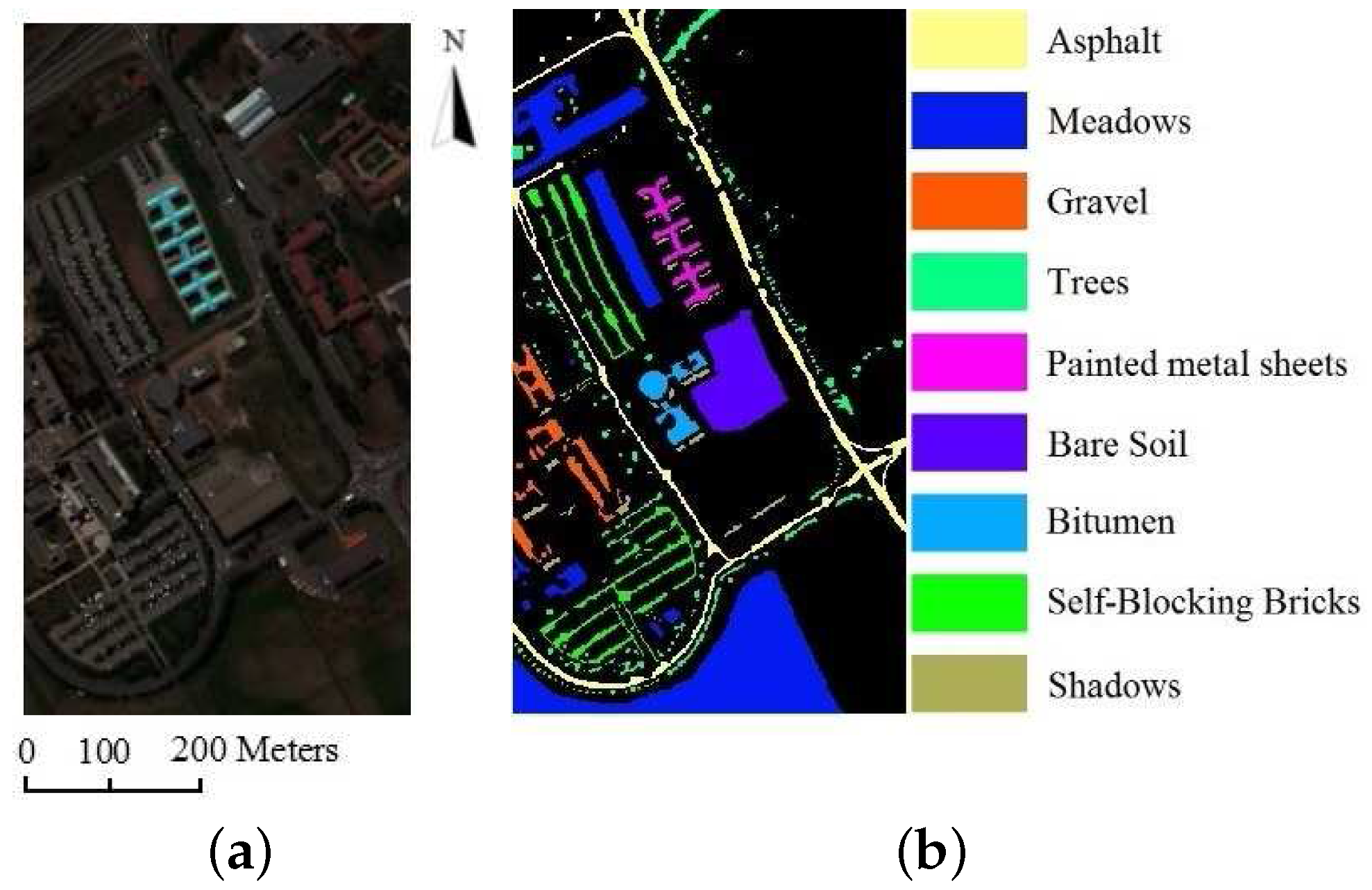
- The second dataset was gathered by the ROSIS sensor over Pavia, Italy. This image has 610 × 340 pixels (covering the wavelength range from 0.4 to 0.9 m) and 115 bands. In our experiments, 12 bands are removed due to the noise. Therefore, there are 103 bands retained. There are nine ground-truth classes, in total 43,923 labeled samples. Figure 6 shows a three-band false color image and the ground-truth map.
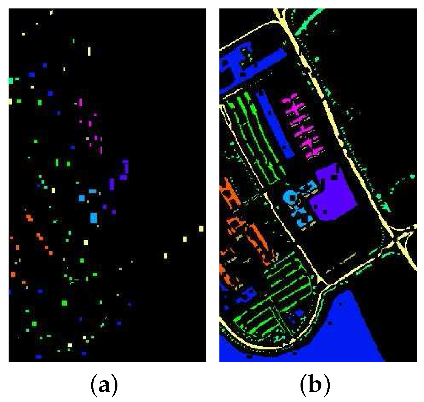
- The third dataset was acquired by the ROSIS-3 sensor in 2003, with a spatial resolution of 1.3 m and 102 spectral bands. This image has nine ground-truth classes and consists of pixels. The number of samples of each class ranges from 2152 to 65,278. There are 5536 training samples and 98,015 testing samples. Note that these training samples are out of the testing samples. A three-band false color image and the ground-truth map are shown in Figure 7.
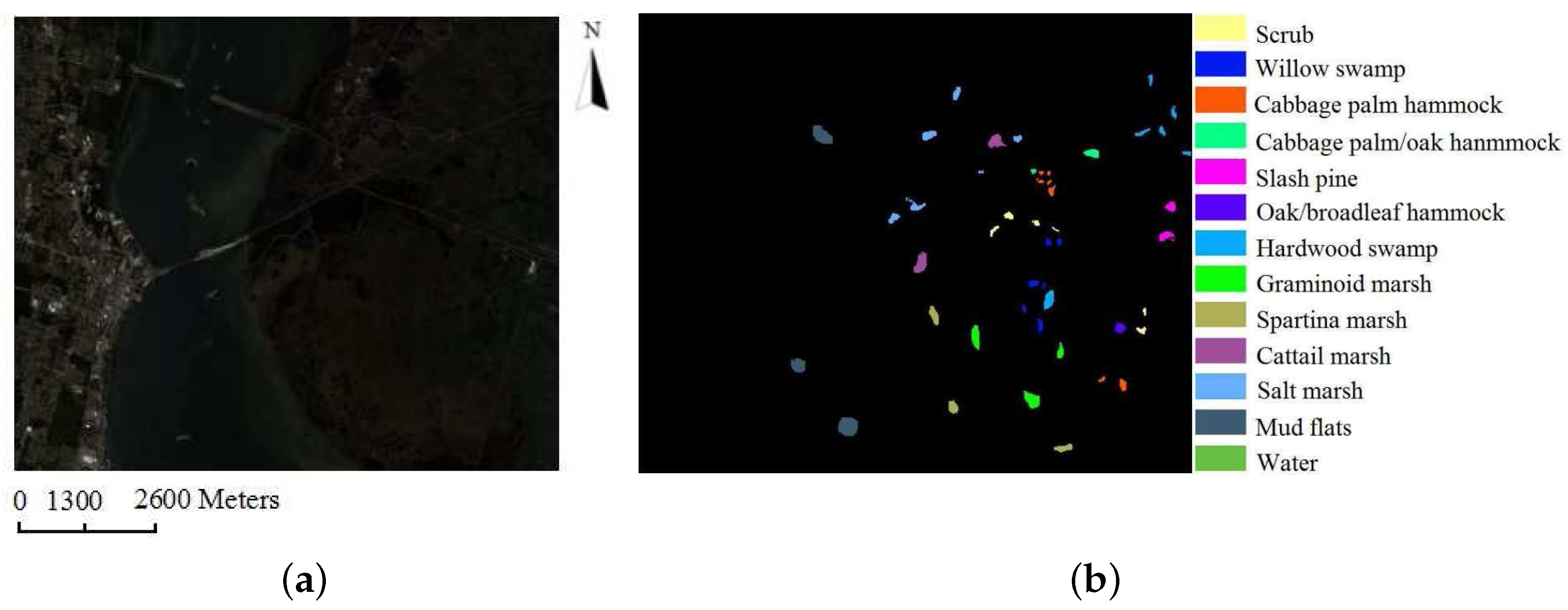
- The last dataset was also acquired by the AVIRIS, but over the Kennedy Space Center, Florida, in 1996. Due to water absorption and the existence of low signal-noise ratio channels, 176 of them were used in our experiments. There are 13 land cover classes with 5211 labeled pixels. A three-band false color image and the ground-truth map are shown in Figure 8.
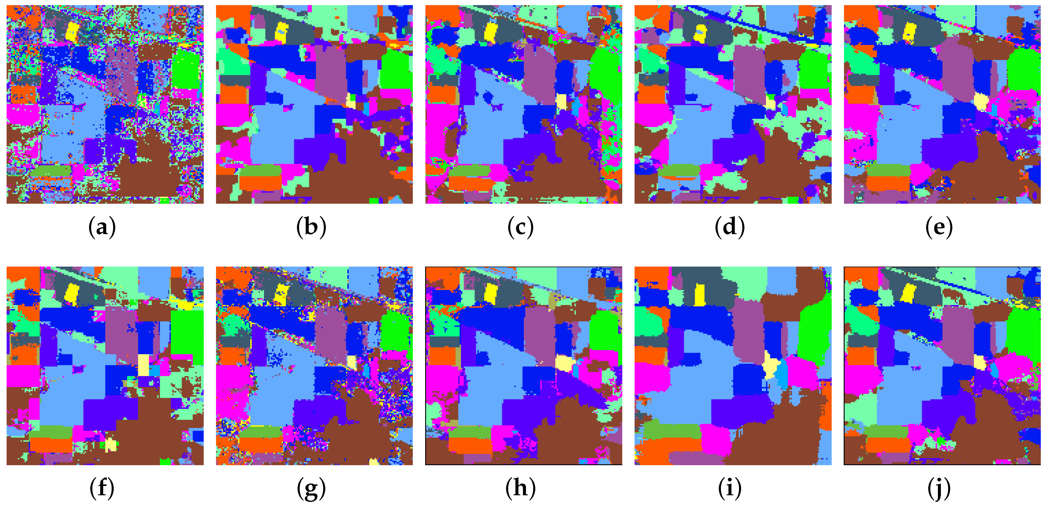
4.2. Experiments with the AVIRIS Indian Pines Dataset
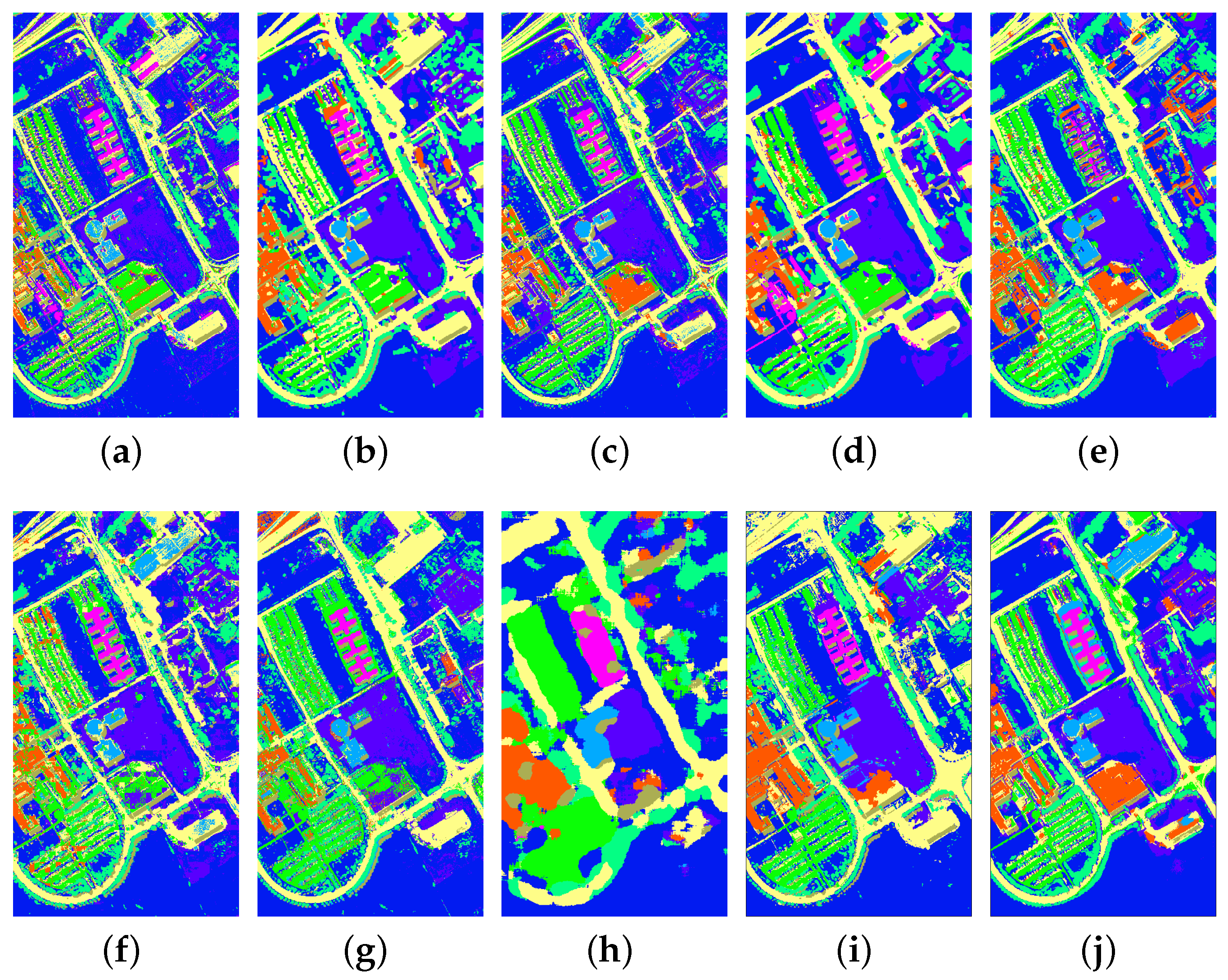
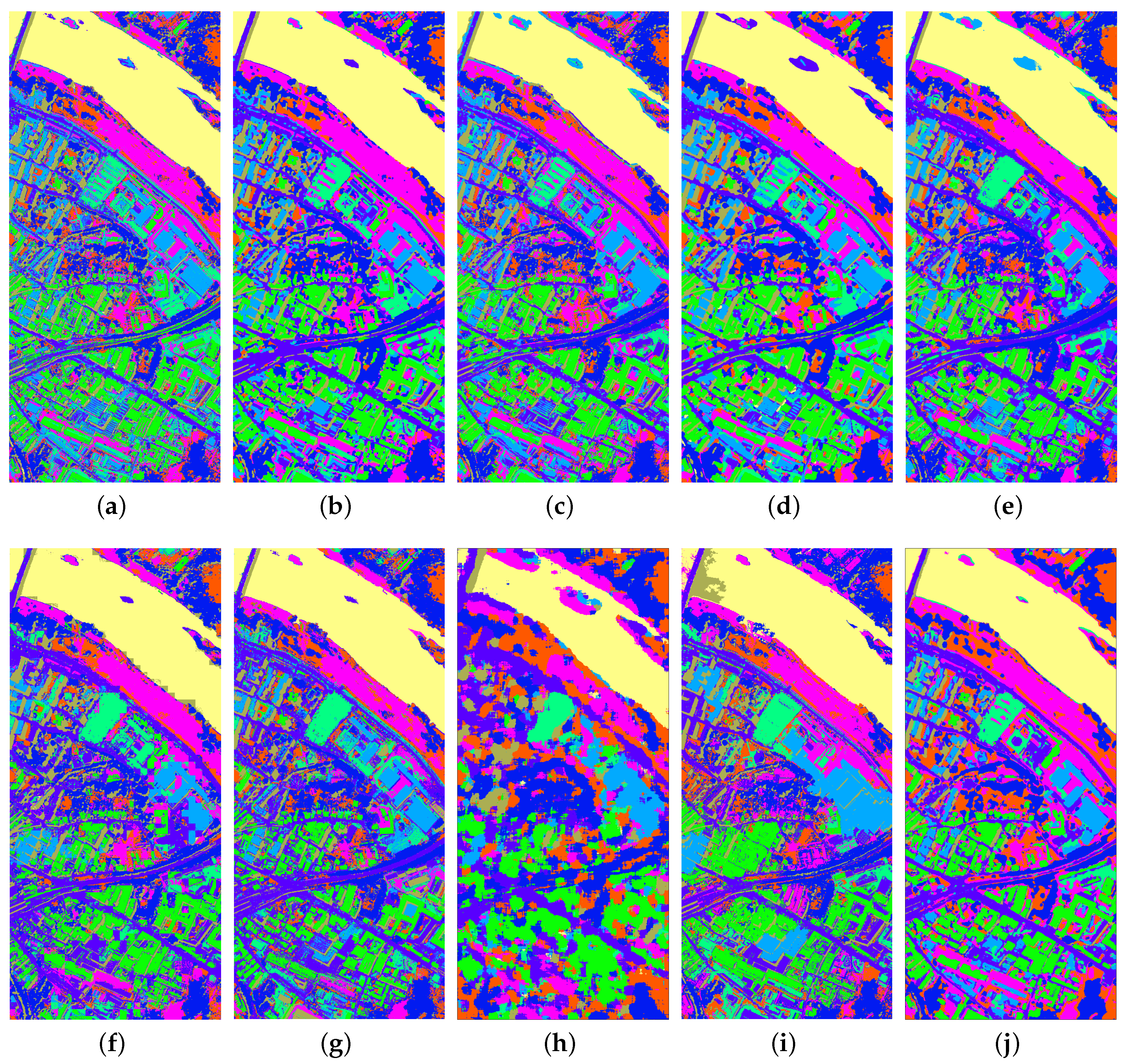
4.3. Experiments with the ROSIS University of Pavia Dataset
4.4. Experiments with the ROSIS Center of Pavia Dataset
4.5. Experiments with the Kennedy Space Center Dataset
4.6. Discussion
5. Conclusions and Future Work
- In SSR, the spectral-spatial features are jointly learned through the template matching. Different template sets may lead to different features. Consequently, it is interesting to design new template learning methods.
- SLN achieves a high classification accuracy by stacking the joint spectral-spatial feature learning units. It is interesting to mathematically analyze and justify its effectiveness according to SSR.
Acknowledgments
Author Contributions
Conflicts of Interest
References
- Fang, L.; Li, S.; Kang, X.; Benediktsson, J.A. Spectral-spatial hyperspectral image classification via multiscale adaptive sparse representation. IEEE Trans. Geosci. Remote Sens. 2014, 52, 7738–7749. [Google Scholar] [CrossRef]
- Zhou, Y.; Peng, J.; Chen, C.L.P. Dimension reduction using spatial and spectral regularized local discriminant embedding for hyperspectral image classification. IEEE Trans. Geosci. Remote Sens. 2015, 53, 1082–1095. [Google Scholar] [CrossRef]
- Ghamisi, P.; Benediktsson, J.A.; Ulfarsson, M.O. Spectral-spatial classification of hyperspectral images based on Hidden Markov random fields. IEEE Trans. Geosci. Remote Sens. 2014, 52, 2565–2574. [Google Scholar] [CrossRef]
- Shi, Q.; Zhang, L.; Du, B. Semisupervised discriminative locally enhanced alignment for hyperspectral image classification. IEEE Trans. Geosci. Remote Sens. 2013, 51, 4800–4815. [Google Scholar] [CrossRef]
- Hou, B.; Zhang, X.; Ye, Q.; Zheng, Y. A novel method for hyperspectral image classification based on Laplacian eigenmap pixels distribution-flow. IEEE J. Sel. Top. Appl. Earth Obs. Remote Sens. 2013, 6, 1602–1618. [Google Scholar] [CrossRef]
- Chang, Y.L.; Liu, J.N.; Han, C.C.; Chen, Y.N. Hyperspectral image classification using nearest feature line embedding approach. IEEE Trans. Geosci. Remote Sens. 2013, 52, 278–287. [Google Scholar] [CrossRef]
- Huang, H.Y.; Kuo, B.C. Double nearest proportion feature extraction for hyperspectral-image classification. IEEE Trans. Geosci. Remote Sens. 2010, 48, 4034–4046. [Google Scholar] [CrossRef]
- Li, W.; Prasad, S.; Fowler, J.E.; Bruce, L.M. Locality-preserving dimensionality reduction and classification for hyperspectral image analysis. IEEE Trans. Geosci. Remote Sens. 2012, 50, 1185–1198. [Google Scholar] [CrossRef]
- Luo, R.B.; Liao, W.Z.; Pi, Y.G. Discriminative supervised neighborhood preserving embedding feature extraction for hyperspectral-image classification. Telkomnika 2012, 10, 1051–1056. [Google Scholar] [CrossRef]
- Tao, D.; Li, X.; Wu, X.; Maybank, S.J. Geometric mean for subspace selection. IEEE Trans. Pattern Anal. Mach. Intell. 2009, 31, 260–274. [Google Scholar] [PubMed]
- Volpi, M.; Matasci, G.; Kanevski, M.; Tuia, D. Semi-supervised multiview embedding for hyperspectral data classification. Neurocomputing 2014, 145, 427–437. [Google Scholar] [CrossRef]
- Zhang, L.; Zhang, Q.; Zhang, L.; Tao, D.; Huang, X.; Du, B. Ensemble manifold regularized sparse low-rank approximation for multiview feature embedding. Pattern Recognit. 2015, 48, 3102–3112. [Google Scholar] [CrossRef]
- Bazi, Y.; Melgani, F. Toward an optimal SVM classification system for hyperspectral remote sensing images. IEEE Trans. Geosci. Remote Sens. 2006, 44, 3374–3385. [Google Scholar] [CrossRef]
- Demir, B.; Ertürk, S. Hyperspectral image classification using relevance vector machines. Geosci. Remote Sens. Lett. 2007, 4, 586–590. [Google Scholar] [CrossRef]
- Huang, G.B.; Zhou, H.; Ding, X.; Zhang, R. Extreme learning machine for regression and multiclass classification. IEEE Trans. Syst. Man Cybern. Part B Cybern. 2012, 42, 513–529. [Google Scholar] [CrossRef] [PubMed]
- Zhang, R.; Lan, Y.; Huang, G.; Xu, Z.; Soh, Y. Dynamic Extreme Learning Machine and Its Approximation Capability. IEEE Trans. Cybern. 2013, 43, 2054–2065. [Google Scholar] [CrossRef] [PubMed]
- Pal, M.; Maxwell, A.E.; Warner, T.A. Kernel-based extreme learning machine for remote-sensing image classification. Remote Sens. Lett. 2013, 4, 853–862. [Google Scholar] [CrossRef]
- Pao, Y.H.; Park, G.H.; Sobajic, D.J. Learning and generalization characteristics of the random vector functional-link net. Neurocomputing 1994, 6, 163–180. [Google Scholar] [CrossRef]
- Chen, C.L.P.; LeClair, S.R.; Pao, Y. An incremental adaptive implementation of functional-link processing for function approximation, time-series prediction, and system identification. Neurocomputing 1998, 18, 11–31. [Google Scholar] [CrossRef]
- Chen, C.P.; Wan, J.Z. A rapid learning and dynamic stepwise updating algorithm for flat neural networks and the application to time-series prediction. IEEE Trans. Syst. Man Cybern. Part B Cybern. 1999, 29, 62–72. [Google Scholar] [CrossRef] [PubMed]
- Ma, J.; Zhao, J.; Tian, J.; Yuille, A.L.; Tu, Z. Robust Point Matching via Vector Field Consensus. IEEE Trans. Image Process. 2014, 23, 1706–1721. [Google Scholar]
- Ma, J.; Zhao, J.; Tian, J.; Bai, X.; Tu, Z. Regularized vector field learning with sparse approximation for mismatch removal. Pattern Recognit. 2013, 46, 3519–3532. [Google Scholar] [CrossRef]
- Chen, C.; Wang, J.; Wang, C.H.; Chen, L. A new learning algorithm for a fully connected neuro-fuzzy inference system. IEEE Trans. Neural Netw. Learn. Syst. 2014, 25, 1741–1757. [Google Scholar] [CrossRef] [PubMed]
- Zhong, Z.; Fan, B.; Duan, J.; Wang, L.; Ding, K.; Xiang, S.; Pan, C. Discriminant Tensor Spectral–Spatial Feature Extraction for Hyperspectral Image Classification. IEEE Geosci. Remote Sens. Lett. 2015, 12, 1028–1032. [Google Scholar] [CrossRef]
- Feng, Z.; Yang, S.; Wang, S.; Jiao, L. Discriminative Spectral–Spatial Margin-Based Semisupervised Dimensionality Reduction of Hyperspectral Data. IEEE Geosci. Remote Sens. Lett. 2015, 12, 224–228. [Google Scholar] [CrossRef]
- Wang, Z.; Nasrabadi, N.M.; Huang, T.S. Spatial-spectral classification of hyperspectral images using discriminative dictionary designed by learning vector quantization. IEEE Trans. Geosci. Remote Sens. 2014, 52, 4808–4822. [Google Scholar] [CrossRef]
- Bernabe, S.; Marpu, P.R.; Plaza, A.; Mura, M.D.; Benediktsson, J.A. Spectral-spatial classification of multispectral images using kernel feature space representation. IEEE Geosci. Remote Sens. Lett. 2014, 11, 288–292. [Google Scholar] [CrossRef]
- Ji, R.; Gao, Y.; Hong, R.; Liu, Q.; Tao, D.; Li, X. Spectral-spatial constraint hyperspectral image classification. IEEE Trans. Geosci. Remote Sens. 2014, 52, 1811–1824. [Google Scholar]
- Fauvel, M.; Tarabalka, Y.; Benediktsson, J.A.; Chanussot, J.; Tilton, J.C. Advances in spectral-spatial classification of hyperspectral images. IEEE Proc. 2013, 101, 652–675. [Google Scholar] [CrossRef]
- Li, J.; Huang, X.; Gamba, P.; Bioucas-Dias, J.M.; Zhang, L.; Atli Benediktsson, J.; Plaza, A. Multiple feature learning for hyperspectral image classification. IEEE Trans. Geosci. Remote Sens. 2015, 53, 1592–1606. [Google Scholar] [CrossRef]
- Bioucas-Dias, J.M.; Plaza, A.; Camps-Valls, G.; Scheunders, P.; Nasrabadi, N.M.; Chanussot, J. Hyperspectral remote sensing data analysis and future challenges. IEEE Geosci. Remote Sens. Mag. 2013, 1, 6–36. [Google Scholar] [CrossRef]
- Camps-Valls, G.; Gomez-Chova, L.; Munoz-Mari, J.; Vila-Frances, J.; Calpe-Maravilla, J. Composite kernels for hyperspectral image classification. IEEE Geosci. Remote Sens. Lett. 2006, 3, 93–97. [Google Scholar] [CrossRef]
- Li, J.; Marpu, P.R.; Plaza, A.; Bioucas-Dias, J.M.; Benediktsson, J.A. Generalized composite kernel framework for hyperspectral image classification. IEEE Trans. Geosci. Remote Sens. 2013, 51, 4816–4829. [Google Scholar] [CrossRef]
- Fauvel, M.; Benediktsson, J.; Chanussot, J.; Sveinsson, J. Spectral and spatial classification of hyperspectral data using SVMS and morphological profiles. IEEE Trans. Geosci. Remote Sens. 2008, 10, 1688–1697. [Google Scholar] [CrossRef]
- Li, J.; Bioucas-Dias, J.M.; Plaza, A. Spectral–spatial classification of hyperspectral data using loopy belief propagation and active learning. IEEE Trans. Geosci. Remote Sens. 2013, 51, 844–856. [Google Scholar] [CrossRef]
- Kang, X.; Li, S.; Benediktsson, J.A. Spectral–spatial hyperspectral image classification with edge-preserving filtering. IEEE Trans. Geosci. Remote Sens. 2014, 52, 2666–2677. [Google Scholar] [CrossRef]
- Li, W.; Du, Q. Gabor-Filtering-Based Nearest Regularized Subspace for Hyperspectral Image Classification. IEEE J. Sel. Top. Appl. Earth Obs. Remote Sens. 2014, 7, 1012–1022. [Google Scholar] [CrossRef]
- Li, W.; Chen, C.; Su, H.; Du, Q. Local Binary Patterns and Extreme Learning Machine for Hyperspectral Imagery Classification. IEEE Trans. Geosci. Remote Sens. 2015, 53, 3681–3693. [Google Scholar] [CrossRef]
- He, L.; Li, Y.; Li, X.; Wu, W. Spectral–Spatial Classification of Hyperspectral Images via Spatial Translation-Invariant Wavelet-Based Sparse Representation. IEEE Trans. Geosci. Remote Sens. 2015, 53, 2696–2712. [Google Scholar] [CrossRef]
- Soltani-Farani, A.; Rabiee, H.R.; Hosseini, S.A. Spatial-aware dictionary learning for hyperspectral image classification. IEEE Trans. Geosci. Remote Sens. 2015, 53, 527–541. [Google Scholar] [CrossRef]
- Sun, L.; Wu, Z.; Liu, J.; Xiao, L.; Wei, Z. Supervised Spectral–Spatial Hyperspectral Image Classification With Weighted Markov Random Fields. IEEE Trans. Geosci. Remote Sens. 2015, 53, 1490–1503. [Google Scholar] [CrossRef]
- Chen, C.; Li, W.; Su, H.; Liu, K. Spectral-spatial classification of hyperspectral image based on kernel extreme learning machine. Remote Sens. 2014, 6, 5795–5814. [Google Scholar] [CrossRef]
- Marpu, P.R.; Pedergnana, M.; Mura, M.D.; Benediktsson, J.A.; Bruzzone, L. Automatic generation of standard deviation attribute profiles for spectral–spatial classification of remote sensing data. IEEE Geosci. Remote Sens. Lett. 2013, 10, 293–297. [Google Scholar] [CrossRef]
- Chen, Y.; Lin, Z.; Zhao, X.; Wang, G.; Gu, Y. Deep Learning-Based Classification of Hyperspectral Data. IEEE J. Sel. Top. Appl. Earth Obs. Remote Sens. 2014, 7, 2094–2107. [Google Scholar] [CrossRef]
- Li, T.; Zhang, J.; Zhang, Y. Classification of hyperspectral image based on deep belief networks. In Proceedings of the 2014 IEEE International Conference on Image Processing (ICIP), Paris, France, 27–30 October 2014; pp. 5132–5136.
- Yue, J.; Zhao, W.; Mao, S.; Liu, H. Spectral–spatial classification of hyperspectral images using deep convolutional neural networks. Remote Sens. Lett. 2015, 6, 468–477. [Google Scholar] [CrossRef]
- Romero, A.; Gatta, C.; Camps-Valls, G. Unsupervised Deep Feature Extraction for Remote Sensing Image Classification. IEEE Trans. Geosci. Remote Sens. 2015, 54, 1349–1362. [Google Scholar] [CrossRef]
- Zhao, W.; Du, S. Spectral- Spatial Feature Extraction for Hyperspectral Image Classification: A Dimension Reduction and Deep Learning Approach. IEEE Trans. Geosci. Remote Sens. 2016, 54, 1–11. [Google Scholar] [CrossRef]
- Chen, Y.; Jiang, H.; Li, C.; Jia, X.; Ghamisi, P. Deep Feature Extraction and Classification of Hyperspectral Images Based on Convolutional Neural Networks. IEEE Trans. Geosci. Remote Sens. 2016, 54, 6232–6251. [Google Scholar] [CrossRef]
- Ghamisi, P.; Plaza, J.; Chen, Y.; Li, J.; Plaza, A. Advanced Supervised Spectral Classifiers for Hyperspectral Images: A Review. IEEE Geosci. Remote Sens. Mag. 2017. accepted for publication. [Google Scholar]
- Zhang, L.; Zhang, L.; Du, B. Deep Learning for Remote Sensing Data: A Technical Tutorial on the State of the Art. IEEE Geosci. Remote Sens. Mag. 2016, 4, 22–40. [Google Scholar] [CrossRef]
- Hinton, G.E.; Osindero, S.; Teh, Y. A fast learning algorithm for deep belief nets. Neural Comput. 2006, 18, 1527–1554. [Google Scholar] [CrossRef] [PubMed]
- Chan, T.H.; Jia, K.; Gao, S.; Lu, J.; Zeng, Z.; Ma, Y. PCANet: A simple deep learning baseline for image classification? arXiv, 2014; arXiv:1404.3606. [Google Scholar]
- Tang, Y.; Xia, T.; Wei, Y.; Li, H.; Li, L. Hierarchical kernel-based rotation and scale invariant similarity. Pattern Recognit. 2014, 47, 1674–1688. [Google Scholar] [CrossRef]
- Li, H.; Wei, Y.; Li, L.; Chen, C.P. Hierarchical feature extraction with local neural response for image recognition. IEEE Trans. Cybern. 2013, 43, 412–424. [Google Scholar] [PubMed]
- Salakhutdinov, R.; Tenenbaum, J.B.; Torralba, A. Learning with hierarchical-deep models. IEEE Trans. Pattern Anal. Mach. Intell. 2013, 35, 1958–1971. [Google Scholar] [CrossRef] [PubMed]
- Ma, X.; Geng, J.; Wang, H. Hyperspectral image classification via contextual deep learning. EURASIP J. Image Video Process. 2015, 2015, 1–12. [Google Scholar] [CrossRef]
- Penatti, O.; Nogueira, K.; Santos, J. Do deep features generalize from everyday objects to remote sensing and aerial scenes domains? In Proceedings of the IEEE Conference on Computer Vision and Pattern Recognition Workshops, Boston, MA, USA, 7–12 June 2015; pp. 44–51.
- Mhaskar, H.; Liao, Q.; Poggio, T. Learning Real and Boolean Functions: When Is Deep Better Than Shallow. arXiv, 2016; arXiv:1603.00988. [Google Scholar]
- Zhang, L.; Zhang, L.; Tao, D.; Huang, X. On combining multiple features for hyperspectral remote sensing image classification. IEEE Trans. Geosci. Remote Sens. 2012, 50, 879–893. [Google Scholar] [CrossRef]
- Zhang, L.; Zhu, P.; Hu, Q.; Zhang, D. A linear subspace learning approach via sparse coding. In Proceedings of the 2011 IEEE International Conference on Computer Vision (ICCV), Barcelona, Spain, 6–13 November 2011; pp. 755–761.
- Yan, S.; Xu, D.; Zhang, B.; Zhang, H.J.; Yang, Q.; Lin, S. Graph embedding and extensions: A general framework for dimensionality reduction. IEEE Trans. Pattern Anal. Mach. Intell. 2007, 29, 40–51. [Google Scholar] [CrossRef] [PubMed]
- Xu, D.; Yan, S.; Tao, D.; Lin, S.; Zhang, H.J. Marginal fisher analysis and its variants for human gait recognition and content-based image retrieval. IEEE Trans. Image Process. 2007, 16, 2811–2821. [Google Scholar] [CrossRef] [PubMed]
- Belhumeur, P.N.; Hespanha, J.P.; Kriegman, D. Eigenfaces vs. fisherfaces: Recognition using class specific linear projection. IEEE Trans. Pattern Anal. Mach. Intell. 1997, 19, 711–720. [Google Scholar] [CrossRef]
- Huang, G.B.; Wang, D.H.; Lan, Y. Extreme learning machines: A survey. Int. J. Mach. Learn. Cybern. 2011, 2, 107–122. [Google Scholar] [CrossRef]
- Pu, H.; Chen, Z.; Wang, B.; Jiang, G.M. A Novel Spatial–Spectral Similarity Measure for Dimensionality Reduction and Classification of Hyperspectral Imagery. IEEE Trans. Geosci. Remote Sens. 2014, 52, 7008–7022. [Google Scholar]
- Li, H.; Xiao, G.; Xia, T.; Tang, Y.; Li, L. Hyperspectral image classification using functional data analysis. IEEE Trans. Cybern. 2014, 44, 1544–1555. [Google Scholar] [PubMed]
- Chen, C.; Li, W.; Tramel, E.W.; Cui, M.; Prasad, S.; Fowler, J.E. Spectral-spatial preprocessing using multihypothesis prediction for noise-robust hyperspectral image classification. IEEE J. Sel. Top. Appl. Earth Obs. Remote Sens. 2014, 7, 1047–1059. [Google Scholar] [CrossRef]
- Fang, L.; Li, S.; Duan, W.; Ren, J. Classification of hyperspectral images by exploiting spectral-spatial information of superpixel via multiple kernels. IEEE Trans. Geosci. Remote Sens. 2015, 53, 6663–6674. [Google Scholar] [CrossRef]
- Chen, Y.; Nasrabadi, N.M.; Tran, T.D. Hyperspectral image classification using dictionary-based sparse representation. IEEE Trans. Geosci. Remote Sens. 2011, 49, 3973–3985. [Google Scholar] [CrossRef]
- Ma, X.; Wang, H.; Geng, J. Spectral–spatial classification of hyperspectral image based on deep auto-encoder. IEEE J. Sel. Top. Appl. Earth Obs. Remote Sens. 2016, 9, 4073–4085. [Google Scholar] [CrossRef]
- Liang, H.; Li, Q. Hyperspectral imagery classification using sparse representations of convolutional neural network features. Remote Sens. 2016, 8, 99. [Google Scholar] [CrossRef]
- Zhang, H.; Li, Y.; Zhang, Y.; Shen, Q. Spectral-spatial classification of hyperspectral imagery using a dual-channel convolutional neural network. Remote Sens. Lett. 2017, 8, 438–447. [Google Scholar] [CrossRef]
- Hutchinson, B.; Deng, L.; Yu, D. Tensor deep stacking networks. IEEE Trans. Pattern Anal. Mach. Intell. 2013, 35, 1944–1957. [Google Scholar] [CrossRef] [PubMed]


| Class Name | SVM | MH-KELM | PCA+Gabor | EPF | MPM-LBP | SADL | MFL | LBP-ELM | SC-MK | SLN |
|---|---|---|---|---|---|---|---|---|---|---|
| Alfalfa | 42.7114.38 | 98.122.07 | 96.462.95 | 100.00.00 | 78.339.68 | 89.5810.67 | 86.467.30 | 97.712.07 | 98.781.29 | 95.003.83 |
| Corn-notill | 74.952.57 | 98.051.14 | 96.041.27 | 97.381.12 | 93.312.73 | 95.180.55 | 91.991.98 | 97.760.84 | 96.831.03 | 98.630.69 |
| Corn-mintill | 67.523.28 | 97.961.57 | 95.151.36 | 97.401.61 | 89.808.17 | 96.481.77 | 93.731.69 | 97.911.07 | 96.041.95 | 99.230.64 |
| Corn | 52.146.37 | 96.712.13 | 94.903.80 | 89.865.52 | 94.247.13 | 87.865.10 | 87.336.34 | 97.764.66 | 95.072.98 | 99.051.27 |
| Grass-pasture | 90.491.07 | 97.251.68 | 94.032.08 | 98.791.02 | 96.242.01 | 97.611.75 | 91.881.63 | 97.402.11 | 95.233.88 | 97.022.29 |
| Grass-trees | 94.390.94 | 99.760.26 | 99.540.43 | 94.843.05 | 99.050.87 | 99.060.64 | 98.380.76 | 99.140.63 | 99.091.18 | 99.900.28 |
| Grass-pasture-mowed | 77.399.35 | 91.747.23 | 98.262.25 | 100.00.00 | 92.1712.43 | 100.00.00 | 87.836.42 | 94.3511.24 | 90.408.68 | 99.964.12 |
| Hay-windrowed | 96.482.09 | 100.00.00 | 99.111.57 | 97.932.70 | 99.640.22 | 100.00.00 | 99.640.32 | 99.910.16 | 100.00.00 | 100.00.00 |
| Oats | 36.1119.64 | 93.895.52 | 91.1117.41 | 30.0048.30 | 52.7836.59 | 84.4432.79 | 48.3313.62 | 92.229.15 | 100.00.00 | 96.1112.30 |
| Soybean-notill | 74.953.26 | 97.971.17 | 95.642.59 | 94.943.44 | 94.453.35 | 95.892.21 | 93.791.79 | 99.050.58 | 94.682.19 | 99.100.83 |
| Soybean-mintill | 83.431.38 | 99.230.25 | 98.130.57 | 90.224.04 | 97.431.50 | 98.271.24 | 98.140.68 | 99.230.52 | 98.900.52 | 99.590.36 |
| Soybean-clean | 65.722.20 | 98.410.71 | 92.342.54 | 95.503.11 | 96.961.49 | 94.582.53 | 91.703.86 | 96.591.36 | 95.651.76 | 98.101.54 |
| Wheat | 95.682.87 | 99.321.45 | 99.320.56 | 100.00.00 | 99.580.22 | 98.890.76 | 99.420.17 | 99.211.78 | 99.570.23 | 99.110.66 |
| Woods | 95.371.31 | 100.00.00 | 98.540.59 | 95.552.14 | 97.781.56 | 98.531.48 | 99.390.34 | 99.880.27 | 99.950.14 | 99.860.21 |
| Buildings-Grass-Trees-Drives | 50.914.91 | 98.450.60 | 93.305.27 | 92.702.37 | 90.704.40 | 98.741.60 | 92.842.73 | 98.772.46 | 98.210.75 | 99.060.79 |
| Stone-Steel-Towers | 85.766.45 | 87.067.72 | 95.183.06 | 95.092.61 | 89.7611.63 | 97.762.11 | 86.246.84 | 94.004.52 | 97.590.57 | 94.713.34 |
| OA | 80.430.54 | 98.650.22 | 96.750.51 | 94.461.45 | 95.611.32 | 97.120.49 | 95.390.44 | 98.630.34 | 97.680.37 | 99.120.19 |
| AA | 74.001.75 | 97.120.97 | 96.061.07 | 91.892.84 | 91.393.01 | 95.812.01 | 90.441.26 | 97.561.28 | 97.250.72 | 98.210.64 |
| κ | 0.7760.006 | 0.9850.003 | 0.9630.006 | 0.9370.017 | 0.9500.015 | 0.9670.006 | 0.9470.005 | 0.9840.004 | 0.9740.004 | 0.9900.002 |
| Data Set | AVIRIS Indian Pines | Pavia University | Pavia University (Fixed Training Set) | Center of Pavia | KSC | |||||||||||
|---|---|---|---|---|---|---|---|---|---|---|---|---|---|---|---|---|
| i | 1 | 2 | 3 | 4 | 5 | 1 | 2 | 1 | 2 | 1 | 2 | 1 | 2 | 3 | 4 | 5 |
| 55 | 55 | 55 | 55 | 55 | 15 | 20 | 15 | 20 | 70 | 80 | 80 | 40 | 40 | 40 | 40 | |
| 25 | 25 | 25 | 25 | 25 | 5 | 5 | 5 | 5 | 7 | 7 | 6 | 6 | 6 | 6 | 6 | |
| 19 | 11 | 11 | 11 | 11 | 17 | 17 | 17 | 17 | 7 | 7 | 13 | 13 | 13 | 13 | 13 | |
| Method | p-Values |
|---|---|
| SVM | 1.594 |
| MH-KELM | 6.999 |
| PCA+Gabor | 5.238 |
| EPF | 2.585 |
| MPM-LBP | 1.703 |
| SADL | 7.860 |
| MFL | 4.265 |
| SC-MK | 1.005 |
| LBP-ELM | 3.400 |
| Class Name | SVM | MH-KELM | PCA+Gabor | EPF | MPM-LBP | SADL | MFL | LBP-ELM | SC-MK | SLN |
|---|---|---|---|---|---|---|---|---|---|---|
| Asphalt | 86.722.59 | 95.571.34 | 91.542.13 | 93.052.57 | 97.381.08 | 92.661.85 | 98.050.81 | 86.341.42 | 96.591.61 | 96.630.91 |
| Meadows | 96.710.66 | 99.770.22 | 99.050.57 | 95.371.80 | 99.450.58 | 98.920.46 | 99.610.15 | 99.230.49 | 98.631.07 | 99.640.62 |
| Gravel | 64.417.13 | 89.155.29 | 80.634.61 | 96.873.67 | 79.023.13 | 74.656.71 | 74.356.36 | 90.212.60 | 96.981.01 | 90.724.19 |
| Trees | 84.931.70 | 90.412.99 | 91.251.97 | 99.460.82 | 90.623.28 | 93.501.60 | 89.782.21 | 61.443.86 | 89.395.88 | 92.861.20 |
| Painted metal sheets | 98.510.80 | 45.626.49 | 97.390.62 | 98.093.84 | 97.520.98 | 99.380.39 | 98.450.86 | 94.336.23 | 99.130.52 | 99.730.18 |
| Bare Soil | 77.704.00 | 97.251.42 | 90.273.96 | 98.520.90 | 93.373.30 | 94.571.81 | 95.041.26 | 99.020.83 | 98.261.44 | 97.381.74 |
| Bitumen | 80.375.24 | 99.250.89 | 85.803.88 | 99.541.09 | 82.959.74 | 77.266.75 | 94.120.86 | 87.857.17 | 93.798.28 | 93.635.32 |
| Self-Blocking Bricks | 83.743.46 | 93.262.60 | 91.553.85 | 87.636.06 | 91.524.53 | 77.732.84 | 93.111.86 | 92.472.36 | 95.512.48 | 95.831.00 |
| Shadows | 95.156.08 | 97.300.76 | 98.260.61 | 96.880.83 | 98.940.70 | 99.140.45 | 91.546.32 | 47.097.74 | 93.696.53 | 87.946.41 |
| OA | 88.770.43 | 95.210.37 | 94.180.33 | 95.061.16 | 95.420.62 | 93.280.50 | 95.830.46 | 91.470.74 | 96.940.66 | 97.140.57 |
| AA | 85.360.65 | 89.730.97 | 91.750.45 | 96.160.75 | 92.311.06 | 89.760.92 | 92.670.99 | 84.221.87 | 95.781.68 | 94.931.27 |
| κ | 0.8510.006 | 0.9370.005 | 0.9230.004 | 0.9350.016 | 0.9400.008 | 0.9120.007 | 0.9450.006 | 0.8870.010 | 0.9600.009 | 0.9620.008 |
| Method | p Values |
|---|---|
| SVM | 1.604 |
| MH-KELM | 8.565 |
| PCA+Gabor | 1.696 |
| EPF | 7.901 |
| MPM-LBP | 5.475 |
| SADL | 1.173 |
| MFL | 4.330 |
| SC-MK | 5.162 |
| LBP-ELM | 3.394 |
| Method | SVM [70] | SVM-CK [70] | SADL [40] | SOMP [70] | LSRC-K [26] | MPM-LBP | SMLR-SpATV | SLN |
|---|---|---|---|---|---|---|---|---|
| Asphalt | 84.30 | 79.85 | 79.17 | 59.33 | 93.86 | 81.66 | 94.57 | 92.48 |
| Meadows | 67.01 | 84.86 | 93.06 | 78.15 | 84.56 | 67.14 | 82.56 | 94.40 |
| Gravel | 68.43 | 81.87 | 85.41 | 83.53 | 74.05 | 74.60 | 81.13 | 76.91 |
| Trees | 97.80 | 96.36 | 95.32 | 96.91 | 98.90 | 95.54 | 95.01 | 96.50 |
| Painted metal sheets | 99.37 | 99.37 | 99.11 | 99.46 | 100.0 | 99.28 | 100.0 | 98.83 |
| Bare Soil | 92.45 | 93.55 | 92.34 | 77.41 | 88.21 | 93.22 | 100.0 | 91.99 |
| Bitumen | 89.91 | 90.21 | 83.00 | 98.57 | 90.93 | 87.87 | 99.17 | 93.78 |
| Self-Blocking Bricks | 92.42 | 92.81 | 92.61 | 89.09 | 97.86 | 90.81 | 98.45 | 97.27 |
| Shadows | 97.23 | 95.35 | 98.29 | 91.95 | 97.99 | 97.48 | 95.45 | 95.47 |
| OA | 79.15 | 87.18 | 90.60 | 79.00 | 88.98 | 78.81 | 90.01 | 93.55 |
| AA | 87.66 | 90.47 | 90.92 | 86.04 | 91.82 | 87.51 | 94.04 | 93.07 |
| κ | 0.737 | 0.833 | 0.875 | 0.724 | 0.855 | 0.732 | 0.872 | 0.914 |
| Method | SVM | MH-KELM | PCA+Gabor | EPF | MPM-LBP | SADL | MFL | LBP-ELM | SC-MK | SLN |
|---|---|---|---|---|---|---|---|---|---|---|
| Water | 98.77 | 97.29 | 98.50 | 100.0 | 99.10 | 98.79 | 99.43 | 86.79 | 96.07 | 99.31 |
| Trees | 91.94 | 96.87 | 92.21 | 99.39 | 94.57 | 92.66 | 87.02 | 86.55 | 87.49 | 98.86 |
| Meadow | 95.21 | 99.95 | 96.44 | 86.78 | 95.83 | 96.63 | 95.83 | 92.22 | 99.38 | 99.72 |
| Brick | 80.62 | 99.70 | 84.58 | 98.28 | 81.94 | 98.32 | 99.46 | 93.28 | 99.88 | 99.16 |
| Bare Soil | 93.84 | 98.67 | 99.42 | 96.64 | 97.75 | 97.91 | 99.43 | 74.92 | 98.99 | 98.97 |
| Asphalt | 95.22 | 99.93 | 98.00 | 77.48 | 95.21 | 95.51 | 95.05 | 83.74 | 95.05 | 98.99 |
| Bitumen | 95.88 | 98.24 | 98.60 | 95.29 | 94.51 | 98.24 | 96.39 | 94.75 | 96.22 | 98.04 |
| Tiles | 99.79 | 99.38 | 99.21 | 100.0 | 99.62 | 98.76 | 99.34 | 90.27 | 99.03 | 99.86 |
| Shadow | 99.95 | 100.0 | 99.95 | 100.0 | 100.0 | 100.0 | 97.23 | 65.99 | 100.0 | 92.69 |
| OA | 97.31 | 97.81 | 97.93 | 97.08 | 97.85 | 98.08 | 98.01 | 86.31 | 95.98 | 99.23 |
| AA | 94.58 | 98.89 | 96.32 | 94.87 | 95.39 | 97.42 | 96.47 | 85.39 | 96.90 | 98.90 |
| κ | 0.951 | 0.961 | 0.963 | 0.948 | 0.961 | 0.965 | 0.964 | 0.772 | 0.929 | 0.986 |
| Method | SVM | MH-KELM | PCA+Gabor | EPF | MPM-LBP | SADL | MFL | LBP-ELM | SC-MK | SLN |
|---|---|---|---|---|---|---|---|---|---|---|
| Scrub | 88.402.57 | 98.761.49 | 98.300.79 | 99.960.13 | 97.841.20 | 95.001.60 | 94.201.80 | 95.304.03 | 92.843.23 | 99.950.13 |
| Willow swamp | 85.004.27 | 98.071.24 | 96.831.71 | 99.660.32 | 91.517.18 | 96.833.29 | 93.071.17 | 94.407.44 | 91.195.49 | 99.310.39 |
| Cabbage palm hammock | 90.742.53 | 99.310.47 | 95.452.70 | 100.00.00 | 98.480.55 | 95.411.76 | 96.281.02 | 99.480.67 | 97.841.26 | 99.740.55 |
| Cabbage palm/oak hammock | 71.854.62 | 88.116.22 | 77.095.67 | 92.425.20 | 76.8312.01 | 87.144.94 | 88.195.64 | 95.954.36 | 91.016.54 | 98.152.45 |
| Slash pine | 66.472.82 | 97.352.97 | 88.164.06 | 98.892.16 | 79.937.87 | 93.313.85 | 94.784.47 | 100.00.00 | 93.018.69 | 100.00.00 |
| Oak/broadleaf hammock | 59.566.81 | 99.950.16 | 90.494.61 | 98.752.44 | 93.635.96 | 95.103.84 | 97.791.75 | 99.411.32 | 95.393.01 | 100.00.00 |
| Hardwood swamp | 90.375.04 | 100.00.00 | 99.381.21 | 88.1212.43 | 99.880.40 | 100.00.00 | 99.750.53 | 100.00.00 | 98.880.71 | 100.00.00 |
| Graminoid marsh | 90.592.84 | 99.330.72 | 94.482.07 | 95.703.05 | 99.331.33 | 97.091.76 | 94.462.11 | 93.259.56 | 96.632.91 | 99.850.24 |
| Spartina marsh | 92.363.30 | 100.00.00 | 99.920.26 | 99.820.22 | 93.476.40 | 98.971.69 | 99.780.18 | 98.401.73 | 99.410.37 | 100.00.00 |
| Cattail marsh | 88.582.66 | 94.120.81 | 96.021.53 | 99.950.11 | 95.252.72 | 91.531.83 | 86.752.28 | 99.261.61 | 99.740.00 | 97.631.91 |
| Salt marsh | 95.661.68 | 99.900.18 | 98.861.00 | 95.452.77 | 98.324.00 | 95.844.68 | 95.304.26 | 99.820.42 | 98.271.25 | 100.00.00 |
| Mud flats | 84.233.97 | 92.742.15 | 95.612.63 | 99.890.27 | 89.214.82 | 92.012.27 | 88.723.77 | 97.891.92 | 96.952.38 | 96.803.06 |
| Water | 98.190.51 | 98.030.29 | 98.590.69 | 100.00.00 | 98.710.61 | 98.820.80 | 98.170.38 | 100.00.00 | 100.00.00 | 98.960.84 |
| OA | 88.390.40 | 97.470.43 | 96.030.41 | 98.450.62 | 94.810.84 | 95.560.38 | 94.520.71 | 97.801.11 | 96.810.48 | 99.160.23 |
| AA | 84.770.61 | 97.360.47 | 94.550.67 | 97.591.27 | 93.261.27 | 95.160.37 | 94.400.73 | 97.941.08 | 96.240.56 | 99.260.19 |
| κ | 0.8710.44 | 0.9720.005 | 0.9560.005 | 0.9830.007 | 0.9420.009 | 0.9500.004 | 0.9390.008 | 97.550.012 | 0.9640.005 | 0.9910.003 |
| Method | p Values |
|---|---|
| SVM | 1.768 |
| MH-KELM | 7.688 |
| PCA+Gabor | 7.769 |
| EPF | 1.086 |
| MPM-LBP | 1.074 |
| SADL | 8.553 |
| MFL | 6.556 |
| SC-MK | 4.398 |
| LBP-ELM | 5.888 |
| Method | Softmax | SVM | KELM |
|---|---|---|---|
| Accuracy (%) | 97.65 | 98.93 | 99.12 |
| Training Time (S) | 19.54 | 0.5565 | 0.0754 |
| Method | 3D-CNN-LR [49] | SDAE [71] | SSDCNN [72] | SSDL [73] | Deep [72] | SLN |
|---|---|---|---|---|---|---|
| Percent of the training samples | 22% | 10% | 10% | 10% | 10% | 10% |
| OA | 97.56 | 98.61 | 96.02 | 91.60 | 97.45 | 99.12 |
| AA | 99.23 | 98.20 | 93.59 | 93.96 | 95.91 | 98.21 |
| κ | 0.970 | 0.982 | 0.947 | 90.43 | 0.964 | 0.990 |
© 2017 by the authors. Licensee MDPI, Basel, Switzerland. This article is an open access article distributed under the terms and conditions of the Creative Commons Attribution (CC BY) license ( http://creativecommons.org/licenses/by/4.0/).
Share and Cite
Wei, Y.; Zhou, Y.; Li, H. Spectral-Spatial Response for Hyperspectral Image Classification. Remote Sens. 2017, 9, 203. https://doi.org/10.3390/rs9030203
Wei Y, Zhou Y, Li H. Spectral-Spatial Response for Hyperspectral Image Classification. Remote Sensing. 2017; 9(3):203. https://doi.org/10.3390/rs9030203
Chicago/Turabian StyleWei, Yantao, Yicong Zhou, and Hong Li. 2017. "Spectral-Spatial Response for Hyperspectral Image Classification" Remote Sensing 9, no. 3: 203. https://doi.org/10.3390/rs9030203