Construction of the Calibration Set through Multivariate Analysis in Visible and Near-Infrared Prediction Model for Estimating Soil Organic Matter

Abstract

The visible and near-infrared (VNIR) spectroscopy prediction model is an effective tool for the prediction of soil organic matter (SOM) content. The predictive accuracy of the VNIR model is highly dependent on the selection of the calibration set. However, conventional methods for selecting the calibration set for constructing the VNIR prediction model merely consider either the gradients of SOM or the soil VNIR spectra and neglect the influence of environmental variables. However, soil samples generally present a strong spatial variability, and, thus, the relationship between the SOM content and VNIR spectra may vary with respect to locations and surrounding environments. Hence, VNIR prediction models based on conventional calibration set selection methods would be biased, especially for estimating highly spatially variable soil content (e.g., SOM). To equip the calibration set selection method with the ability to consider SOM spatial variation and environmental influence, this paper proposes an improved method for selecting the calibration set. The proposed method combines the improved multi-variable association relationship clustering mining (MVARC) method and the Rank–Kennard–Stone (Rank-KS) method in order to synthetically consider the SOM gradient, spectral information, and environmental variables. In the proposed MVARC-R-KS method, MVARC integrates the Apriori algorithm, a density-based clustering algorithm, and the Delaunay triangulation. The MVARC method is first utilized to adaptively mine clustering distribution zones in which environmental variables exert a similar influence on soil samples. The feasibility of the MVARC method is proven by conducting an experiment on a simulated dataset. The calibration set is evenly selected from the clustering zones and the remaining zone by using the Rank-KS algorithm in order to avoid a single property in the selected calibration set. The proposed MVARC-R-KS approach is applied to select a calibration set in order to construct a VNIR prediction model of SOM content in the riparian areas of the Jianghan Plain in China. Results indicate that the calibration set selected using the MVARC-R-KS method is representative of the component concentration, spectral information, and environmental variables. The MVARC-R-KS method can also select the calibration set for constructing a VNIR model of SOM content with a relatively higher-fitting degree and accuracy by comparing it to classical calibration set selection methods.

1. Introduction

Soil organic matter (SOM) is a soil component important to land use and soil fertility [1,2]. SOM is also an important source of carbon circulation due to the large amount of soil organic carbon (SOC) in SOM. Slight changes in SOC will significantly increase atmospheric CO₂ concentrations and exacerbate the greenhouse effect and global climate because of the large amounts of C stored in SOM [3,4]. Hence, predicting the SOM content with a relatively high accuracy is of crucial importance for land management. The visible and near-infrared (VNIR) reflectance spectroscopy technique is commonly used to predict soil content (e.g., SOM content) [5,6]. Related studies mostly focused on exploring the influence of different spectral pre-treatment techniques, and on developing methods for constructing prediction models for SOM. However, the stability and accuracy of the prediction model are considerably affected by methods used for selecting the calibration set, but this has been ignored by most existing studies.

The selection of a calibration set is important in order to ensure the stability and accuracy of the VNIR prediction model [7]. The selection process aims at selecting samples that are representative enough to reveal relationships between component concentrations (e.g., SOM) and VNIR spectra. In most cases, field samplings are not designed to collect specific samples that are representative of the relationships between VNIR spectra and component concentrations. In addition, the design is difficult to establish because the relationships may vary due to the locations and surrounding environments [8,9]. Therefore, we assume that “component concentration representation”, “spectrum representation”, and “environment representation” may be equivalent to “relationship representation”. Environment representation samples are those that are representative of the influence of environmental variables on the relationships between VNIR spectra and component concentrations. The influence of environmental variables on the aforementioned relationships can also be determined as follows. The relationships between VNIR spectra and component concentrations may vary due to the environment. Therefore, scholars must consider specific environmental factors that may influence the relationships during the selection of a calibration set. However, the actual relationships between VNIR spectra and component concentrations remain unknown, thereby complicating the quantification of the impact of environmental factors. Therefore, we assume that the component concentration–related environmental factors are important for the selection of a calibration set. This assumption is practical because some environmental factors can be derived using remotely sensed data, and the relationships between environmental factors and component concentrations can be obtained.

A comprehensive literature review indicates that existing methods for selecting a calibration set can be categorized into three types: methods based on component concentrations, methods based on spectral information, and methods integrating the two formal aspects. Methods based on component concentrations include the concentration gradient method (C method) [10,11] and the clustering mining–based selection method [12]; these methods select the calibration set merely as being representative of the component concentration. A typical method based on spectral information is the Kennard-Stone (KS) method [13]. Other methods, such as the Duplex [14] and GN (global H and neighborhood H) methods [15], are based on the KS method. In these methods, the calibration set selected is representative of reflectance spectra. Based on the two calibration set selection methods, Liu et al. [16] proposed the Rank-Kennard-Stone (Rank-KS) method which maximizes the advantages of the two methods. The calibration set selected by the Rank-KS method is representative of both component concentrations and reflectance spectra.

Notably, the aforementioned types of methods are useful in certain situations, but fail to meet the demands of situations that require the consideration of environmental variables and the spatial heterogeneity distribution of soil samples. Hence, a novel calibration set selection method is proposed in the current work in order to simultaneously consider the SOM content, spectral information, and environmental influence. This proposed method combines the improved multi-variable correlation relationship clustering mining (MVCRC) method and the Rank-KS method. The MVARC-R-KS method is comprised of two phases. In Phase 1, the MVARC method is utilized to adaptively mine clustering zones in which the SOM distribution is significantly influenced by environmental variables; this process integrates the Delaunay triangulation, the Apriori algorithm [17], and a density-based clustering method [18]. In Phase 2, the Rank-KS method is introduced in order to select samples evenly from the clustering zones and the remaining area. The selected calibration sets are then combined and regarded as the final calibration set. The calibration set selected using the MVARC-R-KS method is representative not only of SOM content but also of spectral information and environmental variables.

The rest of this paper is organized as follows. Section 2 describes the study area and materials used. Section 3 introduces the proposed calibration set selection method and the construction of the VNIR-predicting model for SOM content. Section 4 presents the experiments on simulated datasets and real applications to validate the proposed method. Section 5 further discusses the major contributions and results of the current study. Finally, Section 6 presents the conclusions.

2. Study Area and Materials

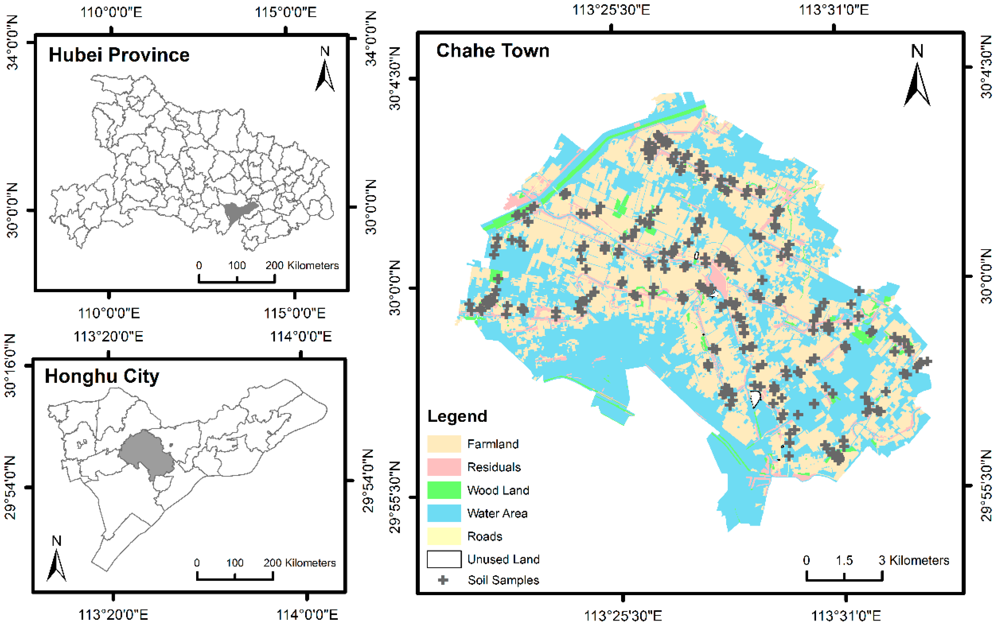
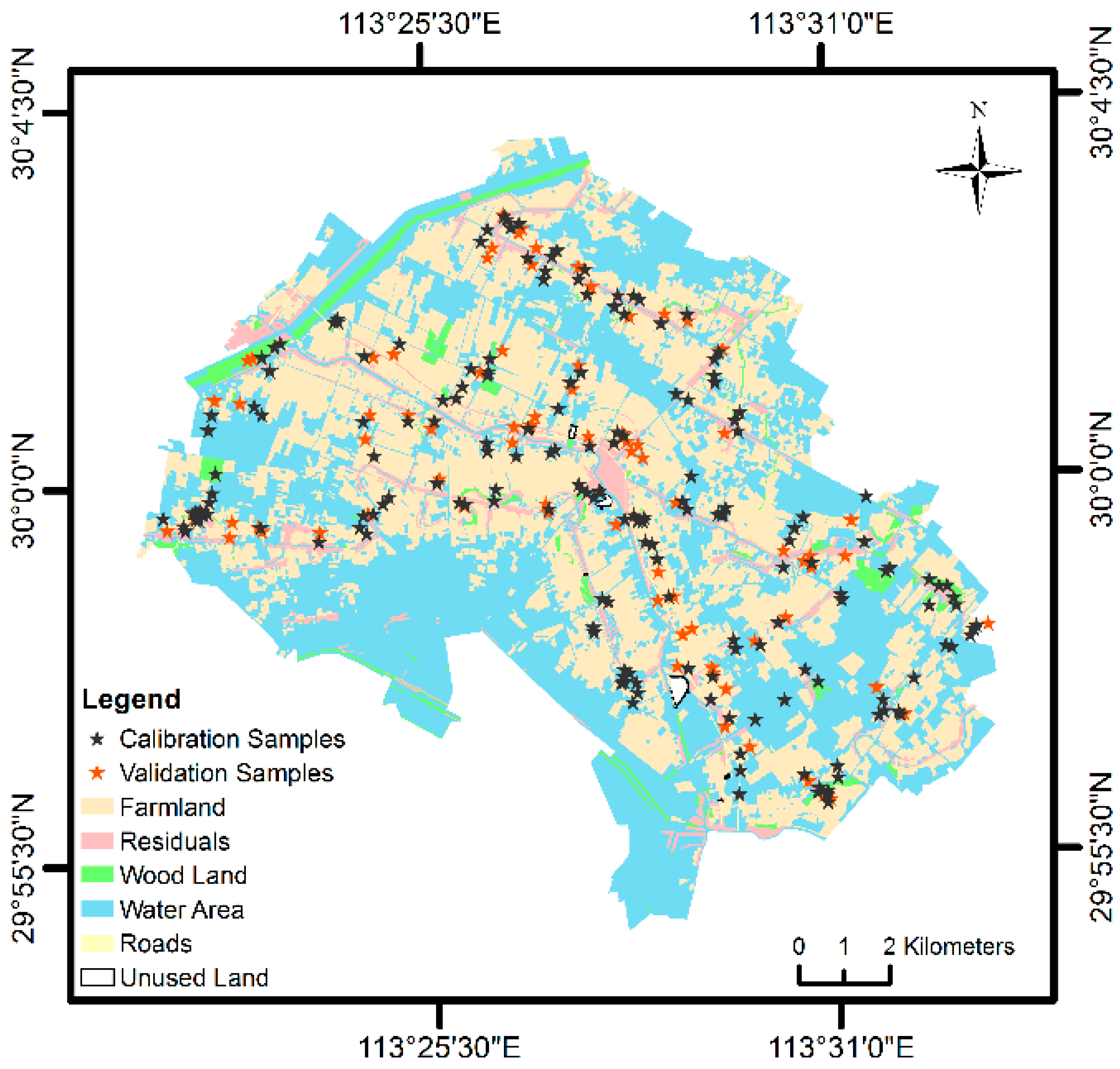
2.1. Study Area

Sampling was conducted in the Jianghan Plain (Hubei Province, China), which is a typical alluvial plain with a humid climate, and is an important agricultural region because of its suitability for multiple crop types. However, in recent years, SOM has been relatively low under the long-term interference of human activities. Hence, dynamic monitoring and prediction of SOM are of important in the land source management of riverfront areas.

A total of 260 topsoil samples (0–30 cm) (Figure 1) were randomly collected from the Jianghan Plain in June 2014. The minimum Euclidean distance between the samples was 100 m. Geographical coordinates were recorded using a handheld global position system (GPS), with a positional error of less than 10 m. All samples were obtained through air-drying, grinding and sieving procedures [19], and then further divided into two portions: One for chemical study and another for spectral measurements.

2.2. Sample Production and Spectral Measurement

SOM content was calculated using Equations (1) and (2).

$$m_1=m\times \frac{w_{dm}}{100}$$

(1)

$$w_{oc}=\frac{\left(A-A_0-a\right)}{b\times m_1\times 1000}\times 100$$

(2)

where $m$ is the mass of the sample, $m_1$ is the mass of the dry matter in the sample, $w_{dm}$ is the percentage of dry matter, $w_{oc}$ is the SOM content (%), $A$ is the absorbance of the digestion solution of the sample, $a$ is the intercept of the calibration curve, and $b$ is the slope coefficient of the calibration curve.$A_0$ is the absorbance in the bland test, which generally uses silica sand or burnt soil as the soil samples for comparison; and details of the calculation of SOM content are given elsewhere (e.g., [4,20]).

The spectral reflectance (350–2500 nm) of the soil samples was measured using an ASD FieldSpec3 portable spectral radiometer. The sampling interval and spectral resolution were set to 1.4 and 3 nm for the 350–1000 nm range, and to 2 and 10 nm for the 1000–2500 nm range. Spectrum scanning was carried out in a dark room, at night, in order to minimize the influence of external light. A standardized white spectra radiometer on a panel was used for reflectance calibration. A white light source, matched with a spectral radiometer with a 45° incident angle, was used. The spectra of the soil samples were measured using the spectral radiometer at a distance of 15 cm, from the probe to the sample surface, and a zenith angle of 90°.

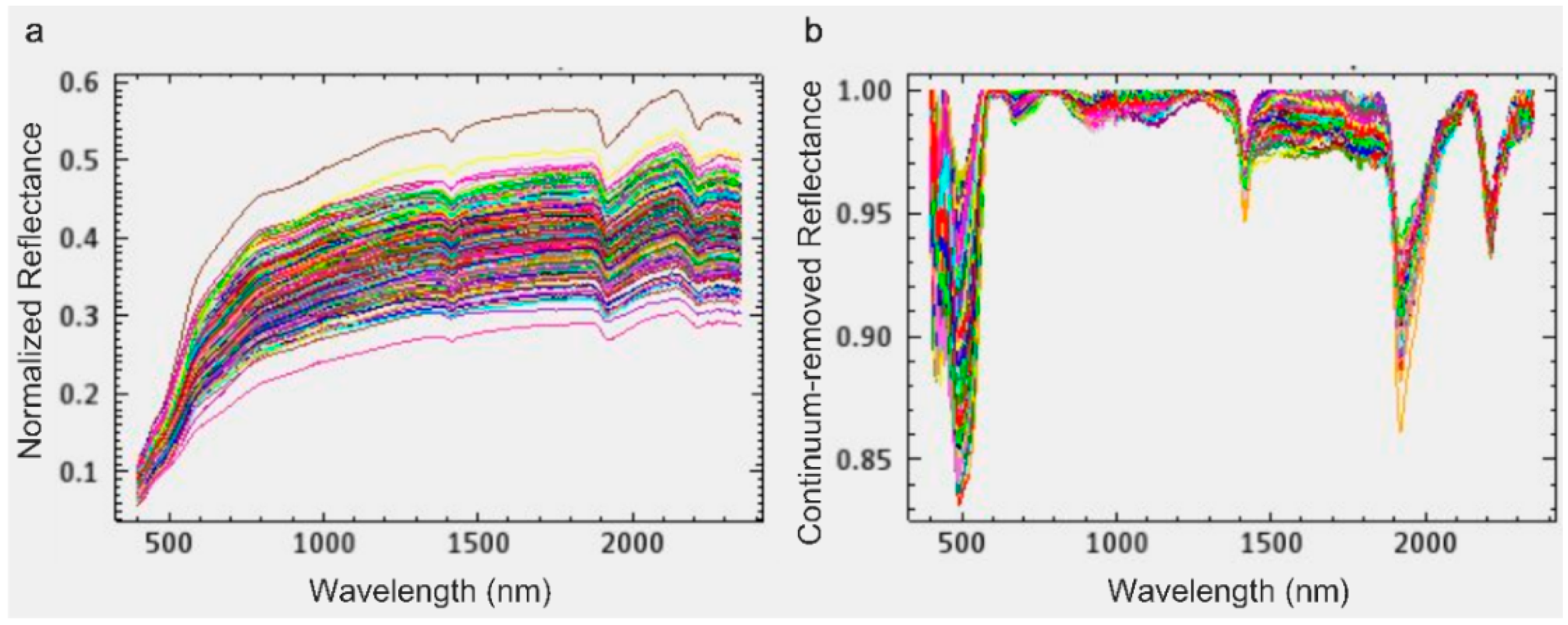
2.3. Spectral Preprocessing

Spectral reflectance is inevitably affected by random noise, baseline drift, and scattering effects because of the impression error from the spectrometer and ambient noise, thereby influencing the stability of the constructed VNIR prediction model. Hence, spectral preprocessing is important and necessary prior to the construction of a prediction model. There are many methods available for spectral preprocessing. In general, they can be classified into two groups: the trial and error method [21,22] and the method based on data characteristics analysis [23,24]. The former is generally time consuming and entails high computation costs, whereas the later seems to be more effective and efficient. Thus, the characteristics of the spectra of the samples are analyzed in order to provide a reference for spectral preprocessing. First, marginal spectra with strong noise are omitted in order to retain those ranging from 400 mm to 2350 mm (Figure 2a). The spectral curves after the continuum-removal are shown in Figure 2b; several small and messy absorption valleys, causing interference in model construction, appear in the VNIR portions of the spectra. Hence, Savitzky-Golay (SG) smoothing should be used for original spectrum smooth denoising. During the spectrum acquisition of solid samples, scattering is unavoidable; hence, the multiplicative scatter correction (MSC) operation and mean center (MC) operation are introduced. The final spectral preprocessing procedures are as follows: SG smoothing, MSC operation, and MC operation, in succession.

2.4. Environmental Variables

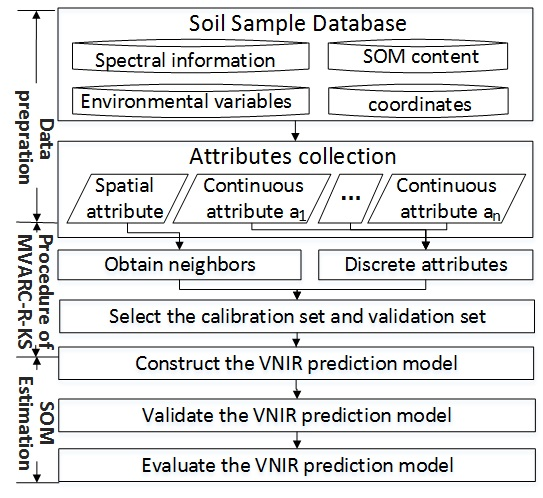
SOM content is considerably influenced by the surrounding environment, and presents spatial heterogeneity [8,9,25]. According to Liu, Guo, Jiang, Zhang and Chen [9], the main environmental variables that affect SOM in the study area include the following three types: (1) soil humidity quantified by the Normalized Difference Moisture Index (NDMI); (2) slope; and (3) distance to residential area.

Environmental variables are calculated based on the Landsat Optical Line Input imagery and ASTER GDEM v2. Details of data processing and calculation of environmental variables are reported in previous studies [9,26].

3. Methods

3.1. Calibration Set Selection Method

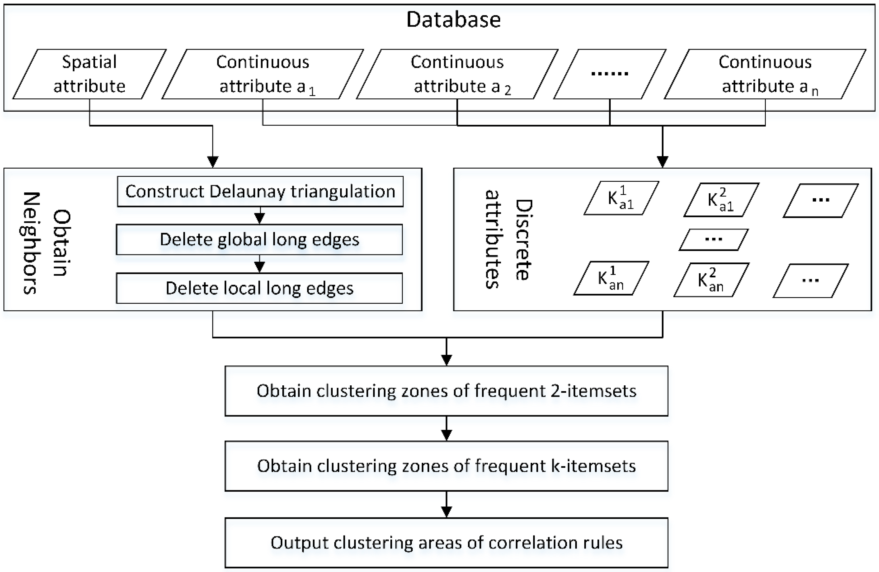
The present study proposes an improved calibration set selection method (MVARC-R-KS), which considers SOM content, spectral information, and environmental variables in selecting the calibration set. The MVARC-R-KS method consists of two phases. In Phase 1, clustering areas with significant association between SOM content and environmental variables are detected by using the MVARC method. In the same detected area, the influence of environmental variables on SOM is regarded as being similar. In addition, the influence of environmental variables on SOM in the remaining zone differs from that in the detected clustering zones. Hence, in Phase 2, a calibration set is selected separately from these zones in order to ensure that it is representative of the environment. The method used for selecting the calibration set is the Rank-KS method, which can select the calibration set, not only being component concentration representative, but also spectrum representative. Phases 1 and 2 are illustrated in Section 3.1.1 and Section 3.1.2, respectively.

3.1.1. MVARC Method

To mine the clustering areas, where distribution of SOM content is significantly associated with environmental variables, an improved multi-variable association relationship clustering mining (MVARC) method is proposed, based on previous studies, which is described in the following paragraph.

To mine association rules at the global level, researchers established various methods, such as Apriori, Fp-Growth, NGEP, and Eclat [27]. Apriori is most widely used in order to recognize correlation rules using support and confidence [17]. However, in real applications, the association rules exhibit significant spatial heterogeneity; hence, mining the association rules at the local level is necessary. Celik et al. [28], Ding et al. [29] and Qian et al. [30] realized local association mining by combing zoning strategies. They first divided the space into several sub-regions, and then the classical global association mining method is used in order to mine the association rules. These methods depend on zoning strategies and cannot be used to mine natural clustering distribution characteristics of association rules. In this regard, Eick et al. [31] and Sha and Li [32] developed a clustering-based association mining framework to detect association rules at the local level. However, a series of parameters needs to be set by default, and the optimal parameters cannot be easily determined. During mining, prior knowledge for providing information for the setting of parameters is always lacking; hence an adaptive association rule clustering mining (MVARC) method is required, and is proposed in this study.

The MVARC method aims to mine clustering zones where consequents (e.g., environmental variables) are considerably affected by antecedents (e.g., SOM content). This method involves two main procedures: The first is to adaptively construct the spatial proximity relationships by adopting the corresponding strategy from adaptive dual clustering algorithm [33]; the second is to mine clustering zones of association rules by integrating the Apriori algorithm [17] and the density-based clustering method [18]. The complete description of the MVARC method can be summarized by the following five steps (Figure 3).

Step 1: Construct the spatial proximity relationships. According to studies [33,34], proximity relationships are obtained by removing the long edges from the constructed Delaunay triangulation.

Step 2: Discretize the continuous attributes (e.g., environmental variables and environmental variables). Association mining method is generally suitable for discrete attributes. If the analyzed attribute is continuous, then it should be discretized to meet the data structure demand of the association mining analysis.

Step 3: Mine the clustering areas of frequent two-item sets (frequent item sets have support greater than minimal support). A density-based algorithm and the Apriori algorithm are integrated in order to mine the clustering areas of frequent two-item sets. Minimal support (MinS) and confidence (MinC), which are the input parameters, are generally set to 0.6 and 0.8, respectively.

Step 4: Mine the clustering areas of frequent k-item sets (k > 2). The clustering areas of frequent k-item sets are iteratively obtained based on clustering areas of frequent two-item sets using overlaying analyses to improve calculation efficiency.

Step 5: Generate rules. This step aims to derive rules with a high confidence from frequent item sets.

The implementation of these steps will now be presented in detail:

Step 1: Construction of spatial proximity relationships.

Delaunay triangulation is powerful for identifying the spatial proximity of objects. According to the study [33], the spatial proximity relationships are adaptively obtained by removing inconsistent edges (long at both global and local levels) from Delaunay triangulation. Objects connected by edges in the modified Delaunay triangulation are considered neighbors. Details of the procedure are provided elsewhere [33].

Step 2: Continuous attribute discretization.

The segment points of the continuous attribute and the number of discretized classes are the most important issues of continuous attribute discretization. The K-means clustering algorithm can obtain the segment points of the continuous attribute considering its natural distribution characteristics. However, the optimal number of discretized classes is difficult to obtain, and the robustness to noise is poor. Hence, an improved K-means algorithm is proposed by developing a discriminant function ($\mathrm{ocf}$ in Equation (3)) for evaluating the optimal discretized classes, and adopting the rule of three standard deviations [33] for dealing with noise.

$$cf\left(r_a,k\right)=\sqrt{\raisebox{1ex}{${{\displaystyle \sum }}_{i=1}^{k}std\_inner\left(r_a\left(clas{s}_i\right)\right)$}\!\left/ \!\raisebox{-1ex}{${{\displaystyle \sum }}_{i=1}^{n}std\_intra\left(r_a\left(clas{s}_i\right)\right)$}\right.}$$

(3)

where $r_a$ is the attribute of objects; $r_a\left(clas{s}_i\right)$ is the label of the discretized class of $r_a$; $n$ is the discretized number; $std\_inner\left(r_a\left(clas{s}_i\right)\right)$ is the standard deviation of $r_a$ of the objects, in which the discretized class of $r_a$ is $clas{s}_i$; and $std\_intra\left(r_a\left(clas{s}_i\right)\right)$ is a similar degree to $r_a$ between objects with different discretized classes. Generally, if the inter-discretized classes are similar and the similarity between intra-discretized classes is large, the discretized number is considered reasonable with a small $ocf\left(r_a,k\right)$ value.

The proposed continuous attribute discretization procedures (Figure 4) can be summarized into the following processes:

(1)

Delete the noise with extreme values. The noise is detected and removed by the rule of three standard deviations.

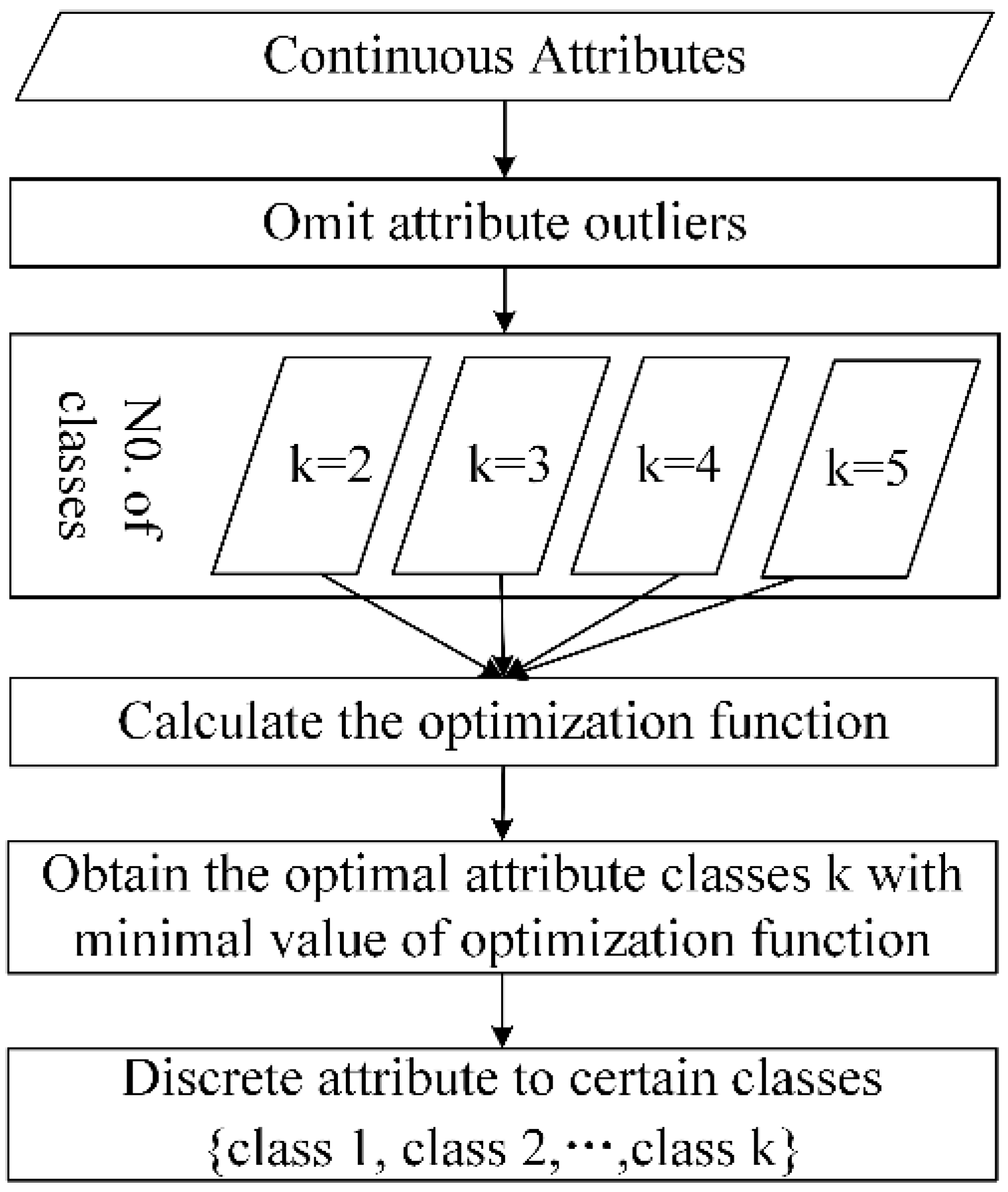
(2)

Choose the optimal number of discretized classes. $ocf$ (Equation (3)) is used to select a suitable number (k) of discretized classes.

(3)

Discrete continuous attribute. The attribute is discretized to k classes by using the K-means algorithm, and the discretized classes are labeled as $\left\{class1,class2,\cdots ,classk\right\}$ according to the attribute mean value of the discretized class, in ascending order.

Step 3: Mining the clustering zones of frequent two-item sets. The procedures are as follows:

(1)

Generate all possible item sets according to antecedents (e.g., SOM content) and consequents (e.g., environmental variables).

(2)

Select an unanalyzed two-item set and label it.

(3)

Calculate clustering cores. For object $p_i$, if its attribute values equal the attribute values of the two-item set, $p_i$ is considered as a potential clustered object. For an potential clustered object $p_i$ its neighboring objects are defined as a neighboring area. In the neighboring area, if the 2 two-item sets are the frequent item sets (the support of the two-item sets is larger than MinS), then the object $p_i$ is defined as the clustering core.

(4)

Select an unlabeled clustering core and label.

(5)

Add the neighboring potential clustered objects of the clustering core and label them.

(6)

Judge the newly added objects. If the object is also a clustering core, iteratively return to (5).

(7)

A cluster of the frequent two-item sets is formed until no more objects can be added. The clustering area of the cluster is set as the minimum circumscribed convex polygon of objects in the cluster. In the present study, the minimum circumscribed convex polygon of the cluster is constructed using the edges of the Delaunay triangulation.

(8)

Implement operations (4) to (7), iteratively. When all the objects have been determined, the clustering zones of the analyzed two-item sets are all recognized.

(9)

Implement operations (2) to (8), iteratively. When all possible two-item sets have been determined, the detection of the clustering zones of all frequent two-item sets is finished.

Step 4: Mining the clustering zones of frequent k-item sets (k > 2).

The clustering zones of possible frequent k/k + 1-item sets are obtained by overlaying the analysis on frequent (k − 1)-item sets and two-item sets. First, the overlaying areas of frequent (k − 1)-item sets and two-item sets are obtained as k/k + 1-item sets. If the zones of the same k/k + 1-item sets are intersected, then these zones are merged.

Taking three-item sets $\left\{r_a\left(class1\right),r_b\left(class1\right),r_c\left(class1\right)\right\}$ as examples. The clustering zones $S\left\{r_a\left(class1\right),r_b\left(class1\right),r_c\left(class1\right)\right\}$ of $\left\{r_a\left(class1\right),r_b\left(class1\right),r_c\left(class1\right)\right\}$ are also the intersection areas of the clustering zones of $\left\{r_a\left(class1\right),r_b\left(class1\right)\right\}$, $\left\{r_a\left(class1\right),r_c\left(class1\right)\right\}$, and $\left\{r_b\left(class1\right),r_c\left(class1\right)\right\}$; additionally, $S\left(\left\{r_a\left(k_1\right),r_b\left(k_2\right)\right\}\right){{\displaystyle \cap }}^{\text{}}S\left(\left\{r_b\left(k_2\right),r_c\left(k_3\right)\right\}\right)\approx S\left(\left\{r_a\left(k_1\right),r_c\left(k_3\right)\right\}\right){{\displaystyle \cap }}^{\text{}}S\left(\left\{r_b\left(k_2\right),r_c\left(k_3\right)\right\}\right)\approx S\left(\left\{r_a\left(k_1\right),r_b\left(k_2\right)\right\}\right){{\displaystyle \cap }}^{\text{}}S\left(\left\{r_a\left(k_1\right),r_c\left(k_3\right)\right\}\right)$. The merged area of the clustering zones is set as the eventual clustering zone when the clustering zones of the same item sets intersect to avoid repeated output of the same clustering areas of the same item sets.

Step 5: Generate clustering zones of rules.

For the clustering zones of item sets, if the number of objects in the clustering zones is less than 0.05 of the total quantity, then these clustering zones are ignored because of weak statistical significance. The confidences of all possible rules from the frequent item sets in the clustering zones are calculated. If the confidence of the rule is larger than MinC, then the rule is judged to present clustering distribution in the corresponding clustering zone. Finally, the clustering zones of rules are trimmed by deleting the sub-rules as follows: When a rule ($r_1$) is the sub-rule (that is, the antecedents and consequents of $r_1$ are all contained by those of $r_2$) of rule $r_2$ and the clustering zone of $r_1$ is contained in the clustering zone of $r_2$, $r_1$ can be deleted because $r_1$ can be inferred by $r_2$.

Clustering zones of rules obtained using the abovementioned five steps have similar association relationship between the antecedents and consequents. Hence, the MVCRC method is conducted by setting environmental variables as antecedents and SOM content as consequent in order to obtain zones with similar values of SOM and environmental variables.

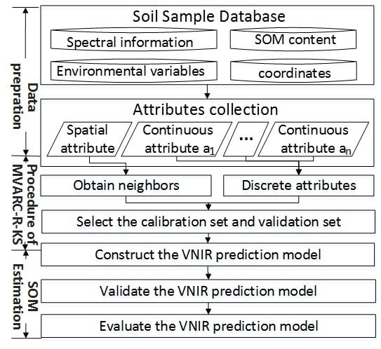
3.1.2. Calibration Set Selection Based on the MVARC-R-KS Method

Several issues should be clarified to select a calibration set by considering SOM gradients, spectral information, and environmental variables: (1) The calibration set selecting scopes are the clustering zones and the remaining zone, obtained using the MVARC method; (2) in the calibration set selection strategy, the calibration set selection operation is conducted on the selecting scopes, separately; the selected calibration sets from these zones emerge as the final calibration set; (3) the Rank-KS method is used to select the calibration set from the selecting scopes; this method is proven effective in selecting representative samples [16]; and (4) the calibration set selecting size is in accordance with Reference [35]; in this study, the accuracy of the prediction model is related to calibration set size. If the size of the calibration set is larger than 60% of the total samples, the result exhibits a relatively high accuracy. Hence, 70% of the samples are selected as the calibration set. If the sample is utilized, not only as a calibration sample, but also as a validation sample, then the degree of reliability will be affected. Hence, the remaining 30% of the samples are utilized as the validation set.

According to the above-mentioned issues, the calibration and validation sets are selected as follows: (1) Clustering zones with a significant association between SOM and environmental variables are obtained by using the MVARC method; (2) the Rank-KS method is utilized at each clustering zone and the remaining zone to select 70% of samples as the calibration set; (3) the selected calibration sets from these zones are combined as the eventual calibration set; and (4) the samples except the calibration set in the study area are labeled as the validation set. The implementation of the selection of calibration set is realized using C# and Matlab 2014a software.

3.2. Construction and Fit Assessment of the VNIR Prediction Model

Partial Least Squares Regression (PLSR) (Equation (4)), which was utilized in this study, is the most widely-used method for constructing a VNIR prediction model. The construction of a prediction model was implemented using the Matlab PLS toolbox.

$$y={\beta }_1{x}_1+{\beta }_2{x}_2+\cdots +{\beta }_k{x}_k$$

(4)

where $y$ is the value of SOM; $x$ represents the spectral value; and ${\beta }_i\left(\mathrm{i}=1,2,\cdots ,k\right)$ is the regression coefficient of $x_i$ and $y$.

The cross-validation procedure (leave-one-out sample) was evaluated. The determination coefficient (${\mathrm{R}}^2$), root mean square error (RMSE), and relative percent deviation (RPD) were applied to measure the performance (including the fitting degree and predictive ability) of the VNIR model. ${\mathrm{R}}_c^2$ and RMSEV reflect the fitting degree of the model construction. If ${\mathrm{R}}_c^2$ is near 1, with a smaller RMSEV, then the stability and fitting degree of the model are considered to be good. The prediction accuracy of the model was examined using ${\mathrm{R}}_p^2$, root mean square prediction error (RMSEP), and RPD. Low RMSEP value and high ${\mathrm{R}}_p^2$ value indicate improved predictive ability of the model. If RPD is less than 1, the model does not have the predictive ability and unsuitable for predicting SOM content. If RPD is between 1 and 1.4, the predictive ability of the model is considered to be poor. If RPD is larger than 1.4 but less than 2, then the model exhibits a preferable predictive ability and can be utilized to predict SOM content. If RPD is larger than 2, then the model is regarded as having a perfect predictive ability [36,37]. The calibration set selection method, which selects the calibration set for constructing a VNIR prediction model with high accuracy, is regarded as being good.

4. Results

The accuracy and feasibility of the proposed method for selecting a calibration set are verified using a simulated dataset and real application. In Section 4.1, a simulated dataset is designed in order to verify the accuracy of the MVARC method. In Section 4.2, the MVARC-R-KS method is utilized in order to select a calibration set for constructing the VNIR model for predicting the SOM content. In addition, classical calibration set selection methods are used to select the calibration set for constructing prediction models. The effectiveness of the MVARC-R-KS method is verified by comparing the stabilities and accuracies of the constructed prediction models based on the calibration set selected.

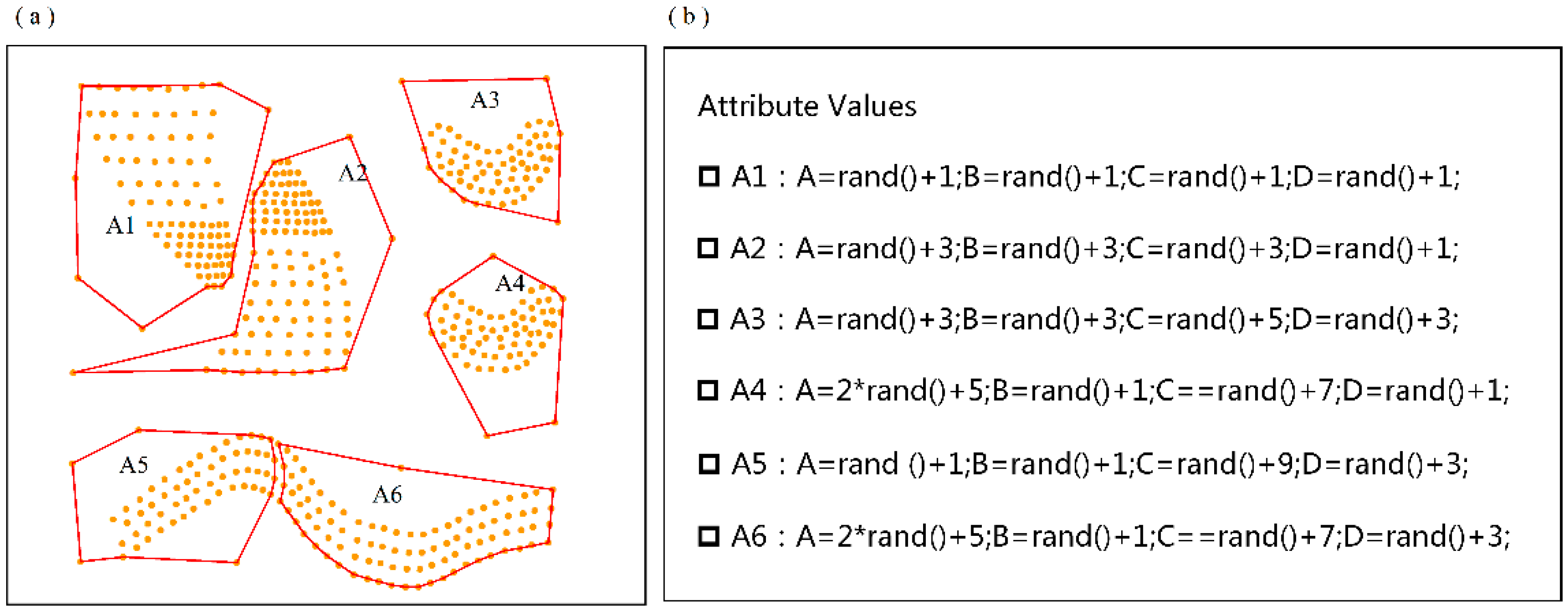
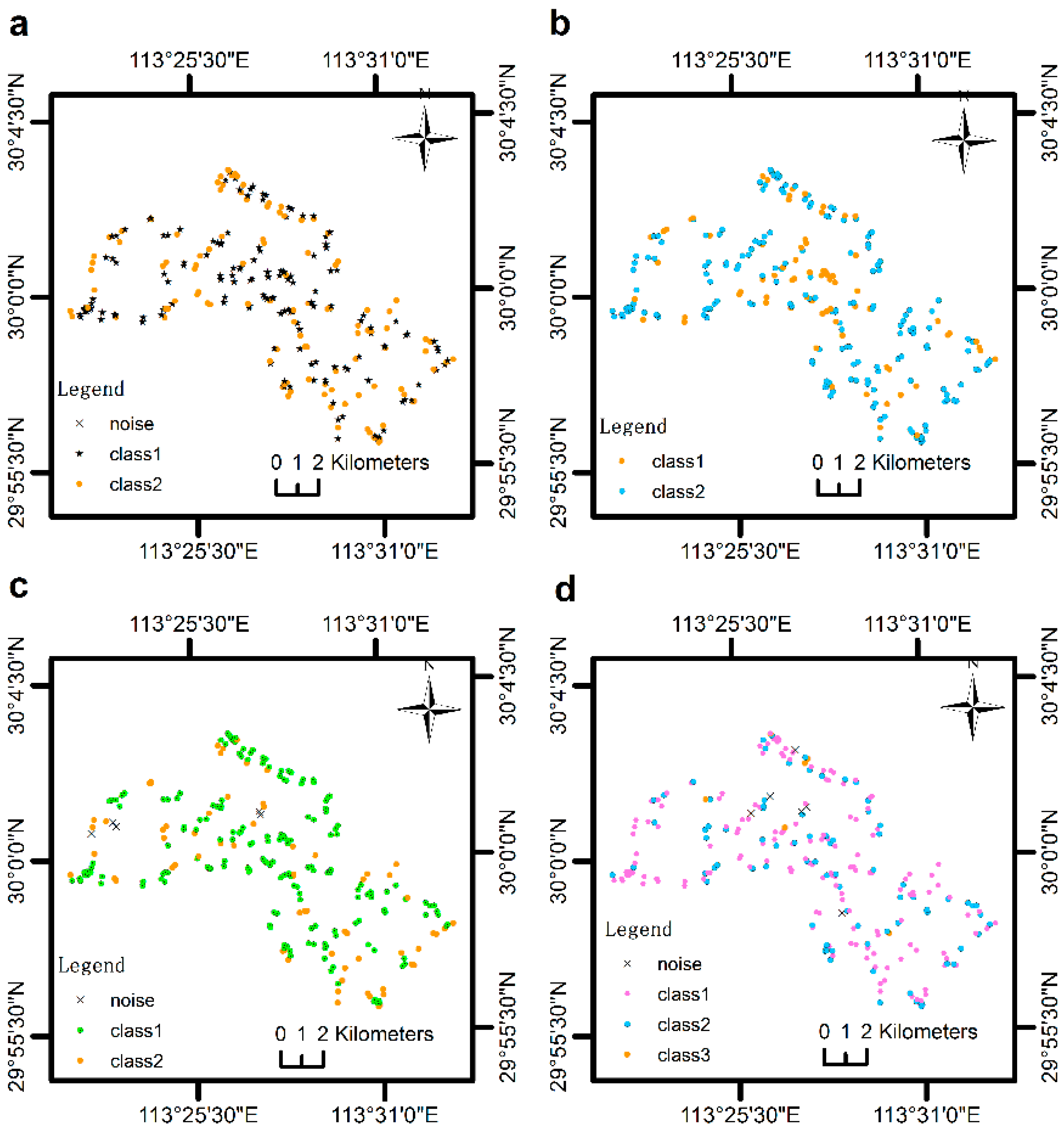
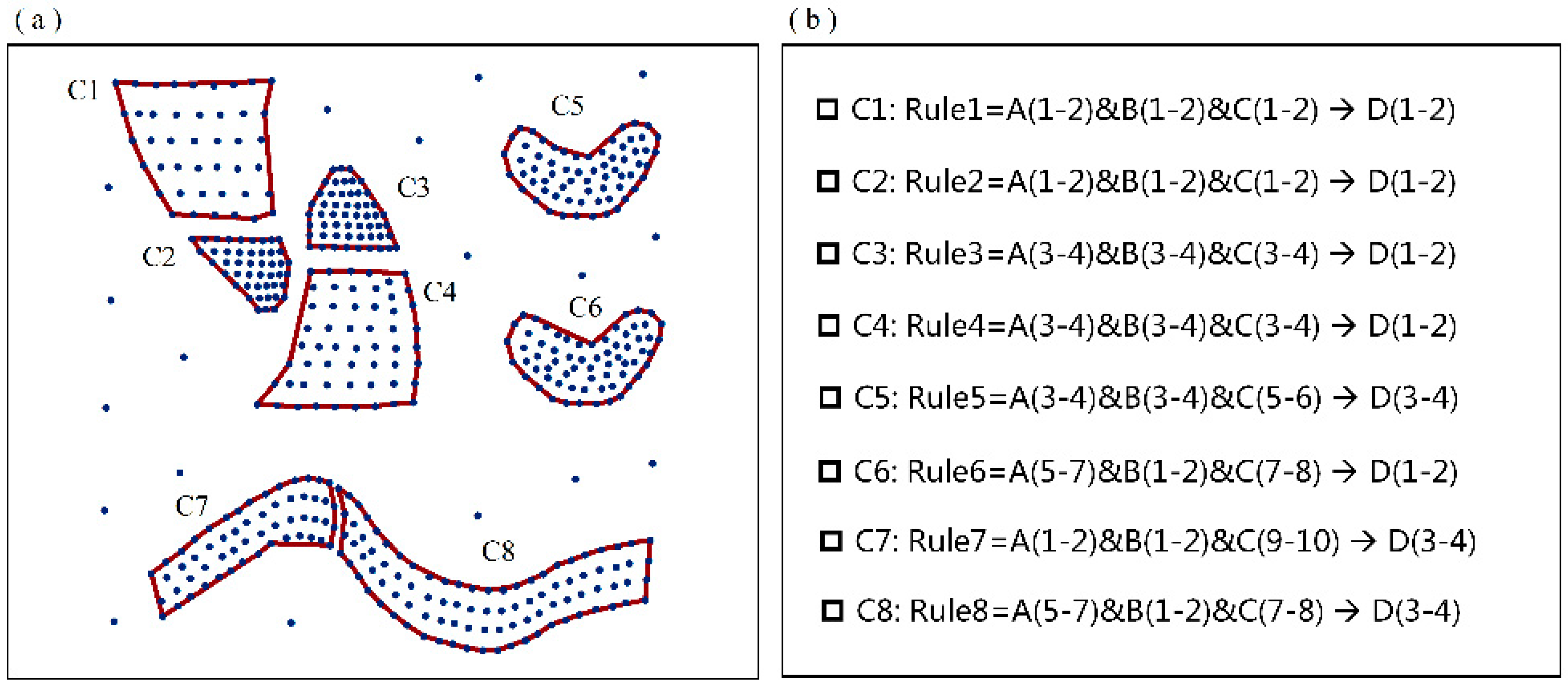
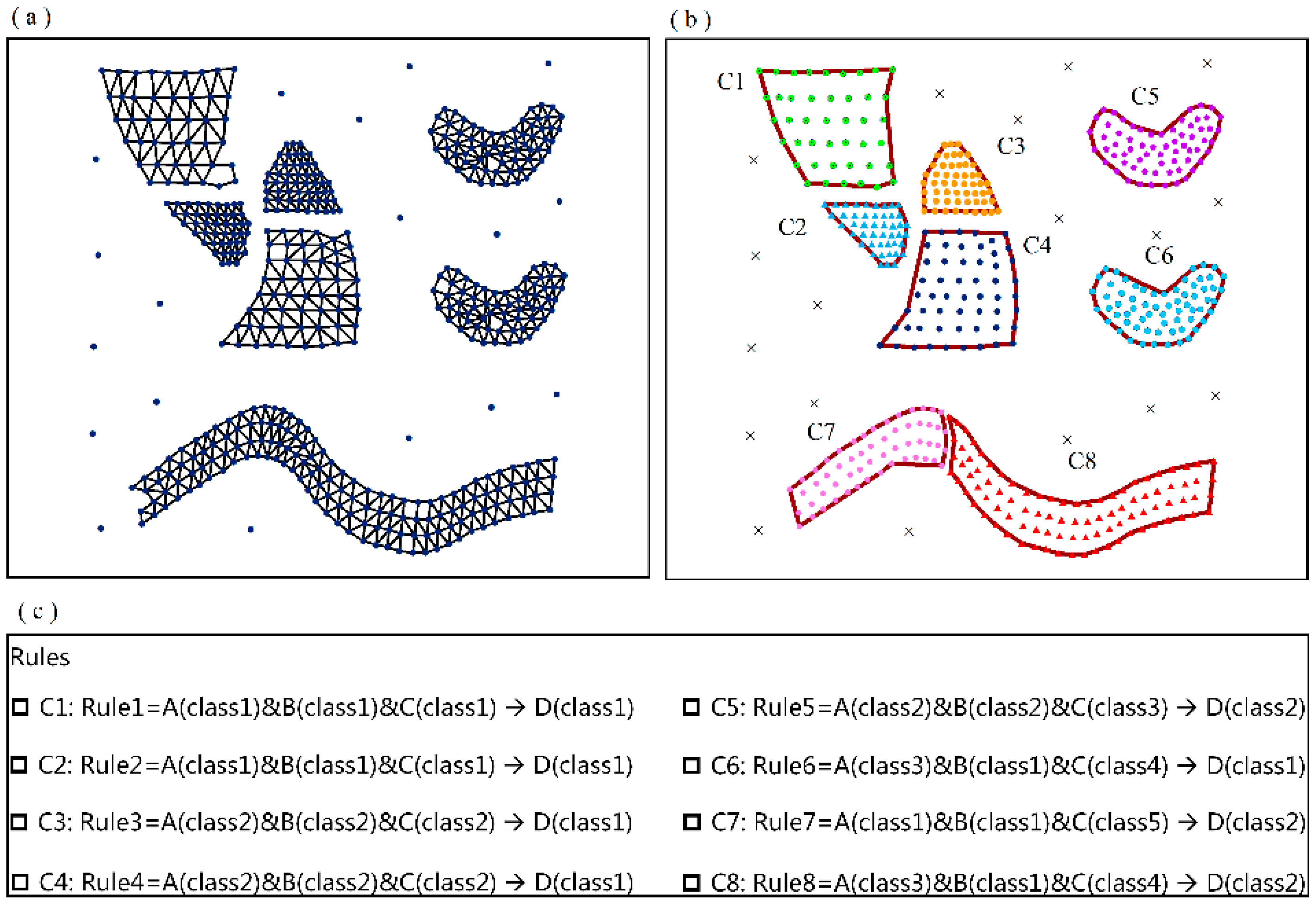
4.1. Validation of the MVARC Method on a Simulated Dataset

A simulated dataset is designed to verify the efficiency and accuracy of MVCRC. The characteristics of the simulated dataset “S” are described as follows:

(1) Objects in S have four continuous attributes: A, B, C and D. The spatial and non-spatial attributes of objects in S are shown in Figure 5.

(2) Several predefined clustering areas of association relationships between the attributes are present in the distribution of spatial and non-spatial attributes of objects. As an example, rules with attributes A, B, and C as antecedents, and attribute D as consequent, are taken. These predefined rules are shown in Figure 6. In real applications, objects tend to be randomly distributed. Hence, objects in the study region have different densities and the predefined clustering areas of rules are zones with arbitrary shapes to be consistent with real applications. In addition, noises in which spatial attribute values are significantly different from those of other objects in the spatial neighborhood exist.

The MVARC method is utilized in order to mine the predefined association relationship clustering zones of S. According to the described calculation procedures of the MVARC method, the spatial proximity relationships, based on the Delaunay triangulation, is first constructed (Figure 7a); then, the continuous attributes are discretized (

Table 1. Discretized classes of attributes A, B, C and D in S.

Attributes	A			B		C					D
Continuous attributes	1–2	3–4	5–7	1–2	3–4	1–2	3–4	5–6	7–8	9–10	1–2	3–4
Discretized attributes	class 1	class 2	class 3	class 1	class 2	class 1	class 2	class 3	class 4	class 5	class 1	class 2

). Finally, the clustering areas of the rules are recognized. The clustering zones and the corresponding rules are shown in Figure 7b,c. Based on the results in Figure 7 and Table 1, the MVARC method can recognize the association relationship clustering zones with a high accuracy, and the MVARC method is suitable for detecting rules with different densities and arbitrary shapes.

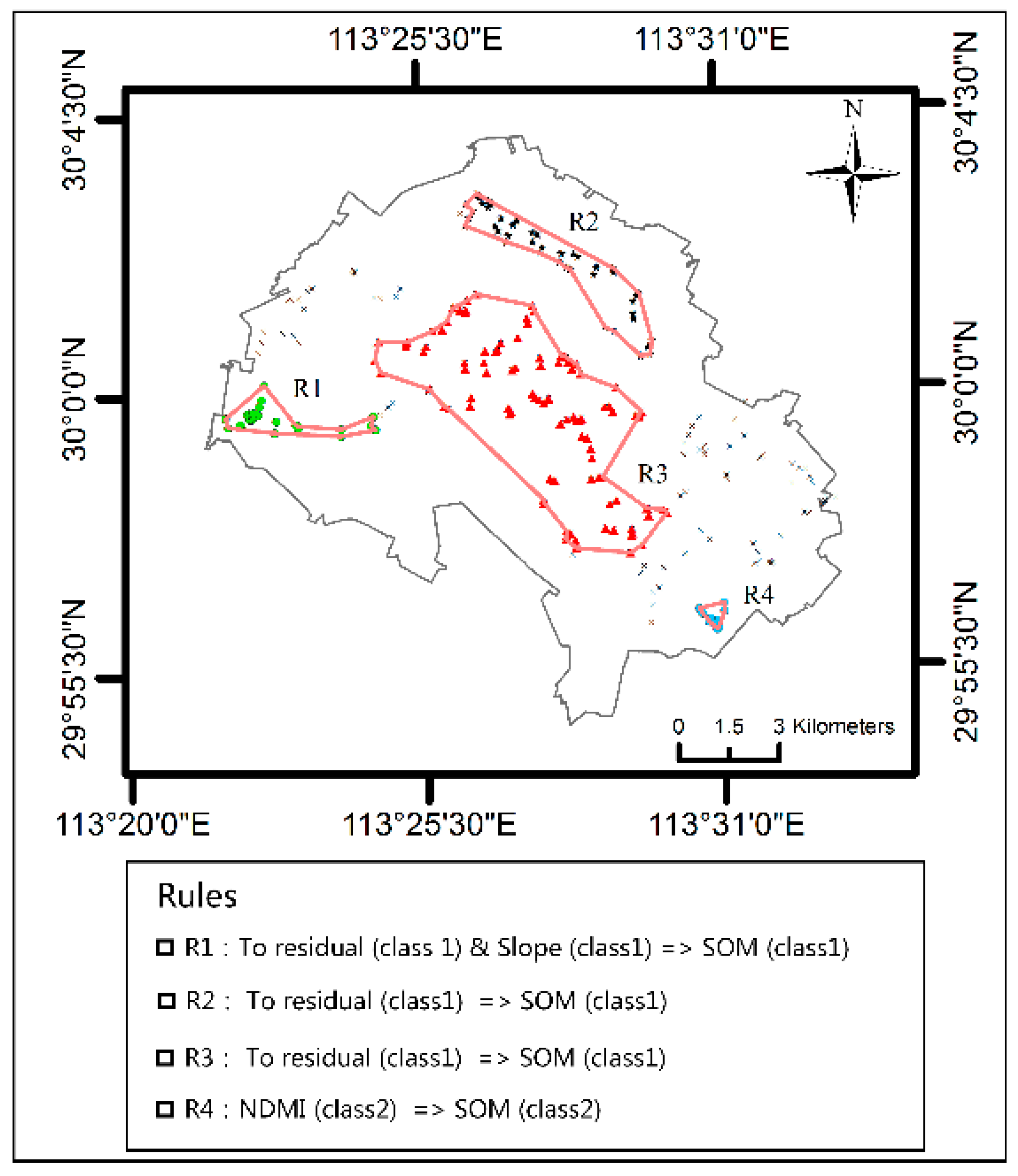
4.2. A Case Study of the MVARC-R-KS Method

In this section, the MVARC-R-KS method is utilized in order to select a calibration set in the VNIR model. The study area and materials given in Section 2 are used as a demonstration region to verify the feasibility and accuracy of the MVCRC-R-KS method. Two main missions are executed as follows. Mission one utilizes the MVARC-R-KS method in order to select the calibration set and construct the VNIR prediction model on the basis of the selected calibration set. This mission aims to verify the feasibility of the proposed MVARC-R-KS method. A detailed description of mission one is given in Section 4.2.1. Mission two compares the MVARC-R-KS method with the classical methods for selecting a calibration set. Both the MVARC-R-KS method and classical methods are used in order to select the calibration set for the VNIR model for predicting the SOM content in the study area. The effectiveness and accuracy of the MVARC-R-KS method are validated by comparing the accuracies and stabilities of the constructed VNIR models based on methods employed for selecting a calibration set.

4.2.1. VNIR Model Based on the Calibration Set Selected Using the MVARC-R-KS Method

Based on the methods in Section 3, the procedures for constructing a VNIR model are as follows: (1) As indicated in Section 3.1.1, the continuous values are discretized and shown in Figure 8. Clustering zones with an association between SOM content and environmental variables, shown in Figure 9, are then obtained by setting environmental variables as antecedents and SOM content as consequents; (2) based on the clustering areas, the Rank-KS method, as described in Section 3.1.2, is utilized in order to select the calibration and validation sets (Figure 10); and (3) the VNIR model is built using the calibration set and is evaluated using the validation set. The fit assessments of the prediction model are shown in

Table 2. Evaluation results of the visible and near-infrared (VNIR) prediction models based on different methods for selecting a calibration set.

Variables	Selection Method	${\mathbf{R}}^2$		RMSE		RPD
		${\mathbf{R}}_{\mathit{c}}^2$	${\mathbf{R}}_{\mathit{P}}^2$	RMSEC (g·kg−1)	RMSEP (g·kg−1)
Values of SOM	C	0.73	0.53	6.39	8.21	1.48
Spectral information	KS	0.78	0.50	5.87	8.82	1.38
SOM values, spectral information	Rank-KS	0.71	0.56	6.51	8.48	1.51
SOM values, spectral information, environmental variables	MVARC-R-KS	0.79	0.70	5.83	6.98	1.81

.

Figure 9 shows that the SOM content is related to environmental variables in the study region, and that there are four main clustering zones. The results indicate that the main residential areas are located in the west, center, and northeast parts of the study region. The main residential areas are consistent with clustering areas R1, R2, and R3. In these areas, the distance to residential area is the main influential environmental factor. Areas near the residential area contain low SOM content, which is also consistent with the study [9]. Liu, Guo, Jiang, Zhang and Chen [9] indicated that the soil near residential areas is seriously affected by frequent human activities, leading to a low SOM content. In addition to the distance to the residential area, another main influential environmental variable is soil humidity quantified by the NDMI. The clustering zone, where SOM is positively correlated with soil humidity quantified by the NDMI, is located in area R5. Areas with high soil humidity can form an anaerobic environment where SOM can be easily accumulated and rarely oxidized.

Based on the clustering zones in Figure 9, the Rank-KS method is utilized in order to select the calibration and validation sets (Figure 10). Samples in the selected calibration sets are representative of the SOM value, spectral information, and environmental variables. The VNIR model, based on the calibration and validation sets, exhibits a high stability and predictive ability (Table 2) and can be utilized to predict SOM content in the riverside region.

4.2.2. Comparison of the MVARC-R-KS Method with Classical Methods for Selecting Calibration Sets

The accuracy of the MVARC-R-KS method is verified by comparing it with classical methods, such as the C method, KS method, and Rank-KS method, which are also utilized in order to select the calibration set for constructing the VNIR model of SOM in the study region. The fit assessments of the prediction models, based on the above-mentioned methods for selecting the calibration set, are shown in Table 2. Results show that several conclusions are drawn according to the assessment strategies in Section 3.2. Compared with the VNIR model based on the calibration set, selected using the MVARC-R-KS method, those based on classical methods exhibit a lower fitting degree and predictive ability. This finding could be due to the interference of the surrounding environment on the soil samples. The MVARC-R-KS method introduces the influence of environmental variables on soil samples and considers the spatial heterogeneity of soil samples. The calibration set selected using the MVARC-R-KS method is representative, not only of SOM values and spectral information, but also of environmental variables, thereby improving the insufficient representation and uneven distribution of the calibration set.

5. Discussion

In this study, an improved calibration set selection method is proposed by integrating the MVARC and Rank-KS methods. The purpose of the proposed MVARC-R-KS method is to select a suitable calibration set that can reveal the relationships between component concentrations (e.g., SOM) and the VNIR spectra well. In the MVARC-R-KS method, the SOM content, spectral information, and the influence of environmental variables are all considered in order to realize the selection of the calibration set. This method is then applied to both simulated datasets and real applications in order to show the feasibility and accuracy. The results (Table 2) show that the VNIR model based on the calibration set, selected using the MVARC-R-KS method, can produce much better estimations than those based on conventional available methods that neglect parts of the aforementioned influencing factors. This result suggests that the SOM content, spectral information and environmental variables are the factors that influence the relationships between VNIR spectra and component concentrations, and should thus be accounted for when selecting the calibration set. The rationality of considering these influencing factors, and the feasibility of the MVARC-R-KS method are discussed in detail as follows.

The distribution of SOM content is significantly correlated with the surrounding environment, particularly with soil humidity quantified by the NDMI, the slope and the distance to the residential area in the study area (Figure 9). Although relationships between environmental variables and SOM content have been recognized and verified by previous studies [8,9,25,38,39], these relationships are ignored during the selection of the calibration set. In the present study, the MVARC-R-KS method introduces the influence of environmental variables to calibration set selection. The effectiveness of the MVARC-R-KS method is described in the following paragraphs.

As indicated in the results (Table 2), the classical C method and KS method do not achieve good results when used to select calibration sets for the construction of VNIR models. These methods either consider component concentrations or spectral information. The Rank-KS method, which considers both component concentrations and spectral information, is demonstrated to be relatively useful for selecting a calibration set to build the VNIR model with ${\mathrm{R}}_p^2=0.56$ and RPD = 1.51 in the study area. These results verify that the VNIR prediction model of SOM content might be biased if an improper calibration set is selected. In order to construct a VNIR model with a high accuracy and robustness, both component concentrations and spectral information should be considered to select the representative calibration set. Although the VNIR model based on the calibration set, selected using the Rank-KS method, shows a predictive ability with acceptable results, its predictive ability is lower than that of the VNIR model based on the calibration set selected using the MVARC-R-KS method. Compared with the Rank-KS method, the MVARC-R-KS method further considers the influence of environmental variables and the spatial heterogeneity of the soil samples. The clustering zones (Figure 9) indicate correlations between the distribution of SOM and environmental variables; such a result is consistent with the results of previous studies [8,9,25,38,39]. Additionally, the distance to the residential area and soil humidity quantified by the NDMI are the major environmental variables influencing the distribution of SOM content in the study area. Furthermore, the influence of the environment on soil samples exhibits significant spatial heterogeneity, which is also why the geographically weighted regression considering spatial heterogeneity has been proven to be effective [9]. The results in Table 2 suggest that the calibration set selected using the MVARC-R-KS method is most representative to reveal relationships between component concentrations (e.g., SOM) and VNIR spectra.

The MVARC-R-KS method selects a representative calibration set by considering multiple variables. To simultaneously consider multiple variables, a hierarchical strategy is generally introduced and proven to be feasible. Hence, in the proposed MVARC-R-KS method, two phases are carried out in succession in order to select a representative calibration set. In Phase 1, the influence of the environment is considered. Association relationship mining methods are useful in mining cause-and-effect relationships; thus, they are considered to be suitable for mining the influence of the environment on soil samples. However, existing association relationship mining methods are not appropriate for adaptively mining relationships with consideration of the spatial heterogeneity of soil samples. Hence, an improved association relationship clustering mining method (i.e., MVARC), is proposed in order to adaptively mine clustering zones in which the influences of the environment on soil samples are similar. In Phase 2, the Rank-KS method, which considers both SOM content and spectral information, is introduced. In order to combine the influence of the environment, the selection strategy of the Rank-KS method is improved as follows: As the clustering zones detected using the MVARC method share similar environmental properties, the environmental properties of the calibration set, if obtained evenly from every zone, become representative. In addition, the environmental properties of the remaining area, except the clustering zones, are different from those of the clustering zones. Hence, the calibration set, evenly selected from the clustering zones and the remaining zone using the Rank-KS method, is regarded as reasonable. The preferable predictive ability of the VNIR model, based on the calibration set selected using the MVARC-R-KS method, indicates the feasibility of the strategy of the proposed MVARC-R-KS method.

In summary, the MVARC-R-KS method is proven to be feasible and accurate. The newly considered environmental variables can be simply calculated based on the Landsat OLI imagery and ASTER GDEM v2. The proposed MVARC-R-KS method could simultaneously consider the internal SOM content, spectral information, and external environmental variables in the calibration set selection, making the VNIR model calibrated from such a calibration set a more widely applicable model for SOM estimation.

6. Conclusions

A novel calibration set selection method called the MVARC-R-KS method is proposed in order to select a calibration set while considering SOM gradients, spectral information, and the surrounding environment. Experiments on the simulated dataset and real application are conducted. Comprehensive comparisons are made between the MVARC-R-KS method and conventional calibration set selection methods. The MVARC-R-KS method exhibits the following advantages: (1) The calibration set selected using the MVARC-R-KS method is representative of the relationships between SOM content and VNIR spectra; (2) the MVARC-R-KS method can be utilized to analyze samples with either discretized attributes or continuous attributes; (3) the proposed MVARC method can adaptively mine association rules at a local level while considering the natural association relationships of objects; and (4) the MVARC-R-KS method can automatically obtain results without sufficient prior knowledge of the dataset.

The MVARC-R-KS method is utilized to select a calibration set for constructing a VNIR model for predicting the SOM content in the riparian areas of the Jianghan Plain in China. The following new findings are obtained: (1) In the study area, the inner component concentrations, VNIR spectra and external environmental variables influence the relationships between SOM content and VNIR spectra; and (2) the fitting degree and accuracy of the prediction model, based on the MVARC-R-KS method, are much better than those obtained with other conventional models for the study area.

Overall, the MVARC-R-KS method can obtain a representative calibration set while considering multiple influencing variables, including the SOM content, environmental variables, and VNIR spectra, parts of which are ignored in conventional methods. The VNIR prediction model based on the calibration set selected using the MVARC-R-KS method shows promise in estimating SOM content. In addition, the MVARC-R-KS method is adaptive and implemented using C# and Matlab 2014a software, which makes the operation convenient.

Future works will focus on the applications of the MVARC-R-KS method. The proposed MVARC method can be used to mine the association relationships and co-location mechanisms of various geospatial phenomena at global and local levels. The MVARC-R-KS method can also serve as a potential technique to select representative calibration sets for calibrating prediction models of various other soil properties, such as Fe content, Cu content, and SOC, in many other areas. Furthermore, spectral reflectance can be reprocessed using the internal soil standard (ISS) method before the application of the MVARC-R-KS method to facilitate data-sharing and comparisons [40].

References

1. Batjes, N.H. Total carbon and nitrogen in the soils of the world. Eur. J. Soil Sci. 1996, 47, 151–163. [Google Scholar] [CrossRef]
2. Mishra, U.; Torn, M.S.; Masanet, E.; Ogle, S.M. Improving regional soil carbon inventories: Combining the IPCC carbon inventory method with Regression Kriging. Geoderma 2012, 189–190, 288–295. [Google Scholar] [CrossRef]
3. Simbahan, G.C.; Dobermann, A.; Goovaerts, P.; Ping, J.; Haddix, M.L. Fine-resolution mapping of soil organic carbon based on multivariate secondary data. Geoderma 2006, 132, 471–489. [Google Scholar] [CrossRef]
4. Wu, C.F.; Wu, J.P.; Luo, Y.M.; Zhang, L.M.; Degloria, S.D. Spatial prediction of soil organic matter content using cokriging with remotely sensed data. Soil Sci. Soc. Am. J. 2009, 73, 1202–1208. [Google Scholar] [CrossRef]
5. Gebbers, R.; Adamchuk, V.I. Precision agriculture and food security. Science 2010, 327, 828–831. [Google Scholar] [CrossRef] [PubMed]
6. Song, H.; Qin, G.; Han, X.; Liu, H. Rapid prediction of soil organic matter by using visible infrared spectral technology. Trans. Chin. Soc. Agric. Mach. 2012, 43, 69–72. [Google Scholar]
7. Daszykowski, M.; Walczak, B.; Massart, D.L. Representative subset selection. Anal. Chim. Acta 2002, 468, 91–103. [Google Scholar] [CrossRef]
8. Qin, Y.; Xin, Z.; Yu, X.; Xiao, Y. Influence of vegetation restoration on topsoil organic carbon in a small catchment of the loess hilly region, china. PLoS ONE 2014, 9, e94489. [Google Scholar] [CrossRef] [PubMed]
9. Liu, Y.; Guo, L.; Jiang, Q.; Zhang, H.; Chen, Y. Comparing geospatial techniques to predict soc stocks. Soil Tillage Res. 2015, 148, 46–58. [Google Scholar] [CrossRef]
10. De Jong, E.; Schappert, H.J.V. Calculation of soil respiration and activity from CO2 profiles in the soil. Soil Sci. 1972, 113, 328–333. [Google Scholar] [CrossRef]
11. Tang, J.; Baldocchi, D.D.; Qi, Y.; Xu, L. Assessing soil CO2 efflux using continuous measurements of CO2 profiles in soils with small solid-state sensors. Agric. For. Meteorol. 2003, 118, 207–220. [Google Scholar] [CrossRef]
12. Guo, Y.; Shi, Z.; Li, H.Y.; Triantafilis, J. Application of digital soil mapping methods for identifying salinity management classes based on a study on Coastal Central China. Soil Use Manag. 2013, 29, 445–456. [Google Scholar] [CrossRef]
13. Technometrics. Index to Contents, Volume 11, 1969. Available online: www.tandfonline.com/doi/abs/10.1080/00401706.1969.10490752 (accessed on 20 December 2016).
14. Technometrics. Advances in Operations Research. Available online: http://amstat.tandfonline.com/doi/abs/10.1080/00401706.1977.10489604 (accessed on 20 December 2016).
15. Wu, J. Research of NIR-Based Technology on Agriculture Products Detection; China Agricultural University: Beijing, China, 2006. (In Chinese) [Google Scholar]
16. Liu, W.; Zhao, Z.; Yuan, H.; Song, C.; Li, X. An optimal selection method of samples of calibration set and validation set for spectral multivariate analysis. Spectrosc. Spectr. Anal. 2014, 34, 947–951. (In Chinese) [Google Scholar]
17. Agrawal, R.; Srikant, R. Fast algorithmsfor mining association rules. In Proceedings of the 20th International Conference on Very Large Databases (VLDB), Santiago, Chile, 12–15 September 1994.
18. Nosovskiy, G.V.; Liu, D.; Sourina, O. Automatic clustering and boundary detection algorithm based on adaptive influence function. Pattern Recognit. 2008, 41, 2757–2776. [Google Scholar] [CrossRef]
19. Guerrero, C.; Wetterlind, J.; Bo, S.; Mouazen, A.M.; Gabarrón-Galeote, M.A.; Ruiz-Sinoga, J.D.; Zornoza, R.; Rossel, R.A.V. Do we really need large spectral libraries for local scale soc assessment with nir spectroscopy? Soil Tillage Res. 2015, 155, 501–509. [Google Scholar] [CrossRef]
20. Liu, Y.; Song, Y.; Guo, L.; Chen, Y.; Lu, Y.; Liu, Y. Comparative analysis of soil organic carbon prediction model based on soil spectral reflectance. Trans. Chin. Soc. Agric. Eng. 2017, 33, 183–191. (In Chinese) [Google Scholar]
21. Liu, Y.; Chen, Y. Feasibility of estimating cu contamination in floodplain soils using vnir spectroscopy—A case study in the le’an river floodplain, china. Soil Sediment Contam. Int. J. 2012, 21, 951–969. [Google Scholar] [CrossRef]
22. Liu, Y.; Chen, Y. Estimation of total iron content in floodplain soils using vnir spectroscopy—A case study in the le’an river floodplain, China. Int. J. Remote Sens. 2012, 33, 5954–5972. [Google Scholar] [CrossRef]
23. Liu, Y.; LU, Y.; Guo, L.; Xiao, F.; Chen, Y. Construction of calibration set based on the land use types in Visible and Near-Infrared (VIS-NIR) model for soil organic matter estimation. Acta Pedol. Sin. 2016, 53, 332–341. (In Chinese) [Google Scholar]
24. Liu, Y.; Jiang, Q.; Fei, T.; Wang, J.; Shi, T.; Guo, K.; Li, X.; Chen, Y. Transferability of a visible and Near-Infrared Model for soil organic matter estimation in riparian landscapes. Remote Sens. 2014, 6, 4305–4322. [Google Scholar] [CrossRef]
25. Li, W.; Zhang, C.; Wang, K. Comparison of geographically weighted regression and Regression Kriging for estimating the spatial distribution of soil organic matter. GISci. Remote Sens. 2012, 49, 915–932. [Google Scholar]
26. Tan, R.; Liu, Y.; Liu, Y.; He, Q.; Ming, L.; Tang, S. Urban growth and its determinants across the Wuhan urban agglomeration, Central China. Habitat Int. 2014, 44, 268–281. [Google Scholar] [CrossRef]
27. Koperski, K.; Han, J. Discovery of Spatial Association Rules in Geographic Information Databases; Springer: Berlin/Heidelberg, Germany, 2000; pp. 47–66. [Google Scholar]
28. Celik, M.; Kang, J.M.; Shekhar, S. Zonal co-location pattern discovery with dynamic parameters. In Proceedings of the Seventh IEEE International Conference on Data Mining (ICDM 2007), Omaha, NE, USA, 28–31 October 2007; pp. 433–438.
29. Ding, W.; Eick, C.F.; Yuan, X.; Wang, J.; Nicot, J.P. A framework for regional association rule mining and scoping in spatial datasets. Geoinformatica 2011, 15, 1–28. [Google Scholar] [CrossRef]
30. Qian, F.; Chiew, K.; He, Q.; Huang, H. Mining regional co-location patterns with knng. J. Intell. Inf. Syst. 2013, 42, 485–505. (In Chinese) [Google Scholar] [CrossRef]
31. Eick, C.F.; Parmar, R.; Ding, W.; Stepinski, T.F.; Nicot, J.P. Finding regional co-location patterns for sets of continuous variables in spatial datasets. In Proceedings of the ACM Sigspatial International Symposium on Advances in Geographic Information Systems, Irvine, CA, USA, 5–7 November 2008; pp. 20–193.
32. Sha, Z. Algorithm of mining spatial association data under spatially heterogeneous environment. Geomat. Inf. Sci. Wuhan Univ. 2009, 34, 1480–1484. (In Chinese) [Google Scholar]
33. Liu, Q.; Deng, M.; Shi, Y.; Wang, J. A density-based spatial clustering algorithm considering both spatial proximity and attribute similarity. Comput. Geosci. 2012, 46, 296–309. [Google Scholar] [CrossRef]
34. Yaolin, L.; Xiaomi, W.; Dianfeng, L.; Leilei, L. An adaptive dual clustering algorithm based on hierarchical structure: A case study of settlements zoning. Trans. GIS 2016. [Google Scholar] [CrossRef]
35. Rana, P.; Gautam, B.; Tokola, T. Optimizing the number of training areas for modeling above-ground biomass with als and multispectral remote sensing in subtropical Nepal. Int. J. Appl. Earth Obs. Geoinf. 2016, 49, 52–62. [Google Scholar] [CrossRef]
36. Shi, T.; Cui, L.; Wang, J.; Fei, T.; Chen, Y.; Wu, G. Comparison of multivariate methods for estimating soil total nitrogen with Visible/Near-Infrared spectroscopy. Plant Soil 2012, 366, 363–375. [Google Scholar] [CrossRef]
37. Viscarra Rossel, R.A.; McGlynn, R.N.; McBratney, A.B. Determining the composition of mineral-organic mixes using UV–VIS–NIR diffuse reflectance spectroscopy. Geoderma 2006, 137, 70–82. [Google Scholar] [CrossRef]
38. Song, X.-D.; Brus, D.J.; Liu, F.; Li, D.-C.; Zhao, Y.-G.; Yang, J.-L.; Zhang, G.-L. Mapping soil organic carbon content by geographically weighted regression: A case study in the Heihe River Basin, China. Geoderma 2016, 261, 11–22. [Google Scholar] [CrossRef]
39. Zeng, C.; Yang, L.; Zhu, A.X.; Rossiter, D.G.; Liu, J.; Liu, J.; Qin, C.; Wang, D. Mapping soil organic matter concentration at different scales using a mixed geographically weighted regression method. Geoderma 2016, 281, 69–82. [Google Scholar] [CrossRef]
40. Kopačková, V.; Bendor, E. Normalizing reflectance from different spectrometers and protocols with an internal soil standard. Int. J. Remote Sens. 2016, 37, 1276–1290. [Google Scholar] [CrossRef]
Figure 1. Location of the study area and layout of soil samples.
Remotesensing 09 00201 g001
Figure 2. (a,b) Original spectra and continuum-removed spectra of soil samples.
Remotesensing 09 00201 g002
Figure 3. Obtaining the spatial clustering distribution of association relationships.
Remotesensing 09 00201 g003
Figure 4. Procedure of continuous attribute discretization.
Remotesensing 09 00201 g004
Figure 5. (a,b) Distribution of the simulated dataset S with its attributes.
Remotesensing 09 00201 g005
Figure 6. (a,b) Predefined association rules between attributes A, B, C (antecedents), and attribute D (consequents), in S.
Remotesensing 09 00201 g006
Figure 7. (ac) Results of the multi-variable association relationship clustering mining (MVARC) method on S.
Remotesensing 09 00201 g007
Figure 8. Discretized values of various continuous attributes: (a) discretized values of the soil organic matter (SOM) content; (b) discretized values of the Normalized Difference Moisture Index (NDMI); (c) discretized values of the distances to the residential area; and (d) discretized values of slopes.
Remotesensing 09 00201 g008
Figure 9. Clustering zones where SOM content is related to the environmental variables.
Remotesensing 09 00201 g009
Figure 10. Distribution of calibration and validation sets selected by the MVARC-R-KS method.
Remotesensing 09 00201 g010