Abstract
The identification of tree species can provide a useful and efficient tool for forest managers for planning and monitoring purposes. Hyperspectral data provide sufficient spectral information to classify individual tree species. Two non-parametric classifiers, support vector machines (SVM) and random forest (RF), have resulted in high accuracies in previous classification studies. This research takes a comparative classification approach to examine the SVM and RF classifiers in the complex and heterogeneous forests of Muir Woods National Monument and Kent Creek Canyon in Marin County, California. The influence of object- or pixel-based training samples and segmentation size on the object-oriented classification is also explored. To reduce the data dimensionality, a minimum noise fraction transform was applied to the mosaicked hyperspectral image, resulting in the selection of 27 bands for the final classification. Each classifier was also assessed individually to identify any advantage related to an increase in training sample size or an increase in object segmentation size. All classifications resulted in overall accuracies above 90%. No difference was found between classifiers when using object-based training samples. SVM outperformed RF when additional training samples were used. An increase in training samples was also found to improve the individual performance of the SVM classifier.
1. Introduction
The identification of tree species through remote sensing provides an efficient and potentially cost-effective way to inventory, protect and manage forest resources [1,2,3,4,5]. Detailed and accurate forest maps are crucial for the preparation and monitoring of fire, drought and other forest disturbances caused by climate change [2,6,7]. Remotely-sensed images contain pixels displaying different surface objects with unique reflectance values, allowing for the discrimination of classes, such as trees and vegetation, based on their spectral signatures [8]. Forest classifications have ranged from more general classifications of forest type (deciduous and coniferous trees) [4,9] to narrower focus classifications of single tree species [1,10,11]. Often, the ability to classify individual species is limited, due to the lack of spectral variance, which helps discriminate small spectral differences between species [12].
The type of imagery is a major factor in classification analysis, as the spatial and spectral resolution can influence the accuracy of a classification. Multispectral images with three to eight bands are commonly used with land cover classifications or forest type (broadleaf, conifer) identification [9,12,13]. In some cases, the limited spectral bands available with multispectral imagery are combined with additional data, including LiDAR, tree heights, shape [14,15], multi-temporal imagery [16] and texture [17].
Hyperspectral images contain multiple (typically between 64 and 256) continuous narrow bands, providing significant levels of detail, which allow for the distinction of fine spectral variations among tree species [18]. Despite the abundance of information contained in hyperspectral imaging, discriminating species within the same genus can be a challenge, often leading to misclassification [3,19]. However, in a comparison between hyperspectral and simulated broadband multispectral classifications in tropical tree species, Clark et al. [12] found that hyperspectral significantly outperformed multispectral. Where multispectral classification fails to capture the slight spectral differences that occur between tree species, data-rich hyperspectral imagery can improve classifications by providing sufficient information to discriminate between spectrally-similar targets [12,15]. This has resulted in the extensive use of hyperspectral imagery for tree species classifications [4,10,20,21].
The high level of data dimensionality in hyperspectral imagery poses a problem for classifications due to the Hughes phenomenon [22]. The increase in spectral bands associated with hyperspectral imagery changes the ratio between the number of training samples and the number of bands, causing the accuracy of the classifier to decrease [23]. To resolve this issue, data reduction through band selection reduces dimensionality without the need to increase training samples [12]. One common method of feature selection in recent years has been the minimum noise fraction (MNF) [4,20,24,25,26,27]. The MNF is a transformation based on two principal component analysis rotations, which first uses principal components to de-correlate noisy data and secondly uses the noise-removed principal components for the final transformation [28]. The resulting MNF bands are ranked by eigenvalue from those containing the highest variance to the highest noise.
Image analysis using pixel-based approaches has been popular [2,26,29], although challenges with this approach have been identified. Issues with pixel-level analysis include shadowed or noise-filled pixels [30], mixed pixels or, for very high resolution imagery, high spectral variety within a class [31].
Object-oriented approaches for classification can offer a more robust method for analysis over pixel-based approaches by providing context to the areas around pixels and a more human-like interpretation of imagery [32]. For classification of trees, object-based segmentations reduce the challenge of crown edge shadowing and spectral variability within pixels that are often found with pixel-based approaches [30]. Object-oriented tree segmentation for tree species classifications commonly occurs on the individual tree crown level [12,19]. Dalponte et al. [30] tested delineation methods with both airborne laser scanning (ALS) and hyperspectral data and determined that neither method was significantly better than the other. When compared to the pixel-based approach, object-based methods have been shown to provide improved classification accuracy in many cases [10,12,20,25].
The support vector machine (SVM) classifier has been increasingly used for complex multi-class problems because it has been found to be better prepared to handle highly dimensional data without an increase in training sample size [33], and some authors even suggest that data reduction is unnecessary for such classifiers [4]. The wide use of the SVM classifier has been apparent in both land cover (forest type) classifications [20,24,27] and tree species classifications [19,21,30], making it one of the more common classifiers used in vegetation classifications.
Support vector machines contain a machine learning algorithm that separates classes by defining an optimal hyperplane between classes, based on support vectors that are defined by training data [33]. In its most basic form, an SVM is a linear binary classifier; however, multi-class strategies have been created that can be applied to complex hyperspectral classifications [23]. While the SVM classifier is seen as a robust method that requires only a small training sample size, the classifier requires trial and error tuning to determine parameters for each classification [33]. The nonlinear SVM with radial basis kernel functions (RBF) requires two parameters to be set. The C parameter determines the amount of misclassification allowed for non-separable training data, enabling the rigidity of training to be adjusted [28]. The gamma parameter is a kernel width parameter that determines the smoothing of the shape of the class-dividing hyperplane [23].
Another non-parametric classifier gaining wider use is the random forest classifier (RF) as developed by [34]. Random forest is an ensemble-based machine learning algorithm that uses multiple decision tree classifiers to vote on a final classification. Only a few parameters are required, including N (number of trees) and m (number of predictor features) [13]. With minimal parameter settings and few variables, random forest has been found to require less complex computations and running time than other classifiers, as well as having high classification accuracy in especially intricate models [35]. Random forest has been suggested as an alternate classifier to SVM for multi-class problems, as it requires fewer parameters than SVM [13].
The objective of this research is to compare and examine the performance of two state-of-the-art classifiers, random forests and support vector machines, for tree species classification in a forest setting with a non-homogenous tree species distribution. A comparative classification approach is used to assess the performance of the two classifiers, with additional consideration for the influence of training sample size and object-based segmentation size on the individual performance of the individual classifiers. To further explore the impact of training sample size, pixel-based and object-based reflectance values are used.
2. Materials and Methods
2.1. Study Area
The study area consists of Muir Woods National Monument and adjacent Kent Creek Canyon, located in Marin County, CA, about 15 miles north of San Francisco, CA (Figure 1). The parks are managed by the U.S. National Parks Service and the California State Parks, respectively. Both parks occur within the Redwood Creek watershed, which extends steeply to the Pacific Ocean, roughly 5.5 miles to the south. The park’s close proximity to the colder ocean water creates fog, resulting in fog drip, which helps support the redwood forest ecosystem [36]. In 1908, Muir Woods became a National Monument, protecting the remaining old growth redwoods. With over 1 million visitors in 2014, efforts within Muir Woods are being made to minimize high visitor impacts, including erosion, noise-pollution and traffic [37,38].
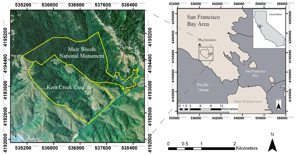
Figure 1.
Muir Woods National Monument and Kent Creek Canyon are located along the California coastal range in the San Francisco Bay Area.
Muir Woods National Monument occupies 2.25 square kilometers in the upper reaches of the Redwood Creek Watershed, where old growth coast redwoods (Sequoia sempervirens), Douglas fir (Pseudotsuga menziesii) and California bay laurel (Umbellularia californica) dominate the forest canopy. The extent of tan oak (Lithocarpus densiflorus) and big leaf maple (Acer macrophyllum) are limited, but occupy both the canopy and understory. Although some of the redwood trees in the area are over 600 years old, the forest contains trees of varying ages [39].
To the west of Muir Woods National Monument is the smaller Kent Creek Canyon, part of Mt. Tamalpais State Park. The Kent Creek area exhibits drier conditions than Redwood Canyon. In this area, bay laurel, coast live oak (Quercus agrifolia) and Douglas fir are more abundant, while the extent of coast redwood is limited. Kent Creek Canyon includes extensive non-forested areas containing coyote brush and grassland. In both parks, arroyo willow (Salix lasiolepis) and red alder (Alnus rubra) corridors line Redwood Creek, while California buckeye (Aesculus californica) is found along Muir Woods Road and around the Muir Woods main parking lot. Within the boundaries of Muir Woods National Monument, a small grove of non-native eucalyptus (Eucalyptus globulus) sits in the eastern edge of the park in the Canyon de Camino area. The eucalyptus grove was planted before the land was acquired as part of the park [37].
2.2. Remote Sensing Data
Acquisition of remote sensing data for this project occurred through the Golden Gate LiDAR Project [40] (Table 1). Airborne hyperspectral data were acquired using an AISA Eagle sensor with a 23-mm lens. The sensor was flown at an altitude of 2286 meters with a FWHM (bandwidth) of approximately 4.6 nm. Multiple flight lines were flown, out of which four flight line images were ultimately selected based on time of day taken, the spatial coverage of the study area and the temporal proximity between images. The LiDAR and hyperspectral data were acquired concurrently. A minimum LiDAR point density was planned for 4 points/m2, but additional flight lines flown over Muir Woods National Monument densified the LiDAR points, resulting in an average raw point density of 8 points/m2. In Kent Canyon, the raw point density averaged 4 points/m2, but areas with deep canyons generally resulted in a point density between 7 and 8 points/m2 [41].

Table 1.
Hyperspectral imagery and LiDAR were collected as part of the Golden Gate LiDAR project.
2.3. Pre-Processing
The LiDAR point data were classified into ground, canopy and building points, and QA/QC (quality assurance/quality control) was completed to remove noise points using LP360 software [42]. A digital elevation model (DEM) and canopy height model (CHM) were created with a spatial resolution of 0.5 m using a regularized spines with tension interpolation from the LiDAR data using open source software [43]. This spatial resolution was selected after a comparison of the 0.5-m and 1-m DEM/CHM showed additional topographic and canopy detail in the 0.5-m datasets.
Most initial pre-processing of the hyperspectral data occurred separately from this study as part of the Golden Gate LiDAR project and included radiometric corrections from digital numbers to reflectance, geometric calibration and orthorectification [41]. Additional processing was completed using ENVI 5.1 [28]. Atmospheric corrections were applied to each flight line image using the fast line-of-sight atmospheric analysis of spectral hypercubes (FLAASH) algorithm, converting the image from radiance to reflectance. Hyperspectral flight lines were clipped as close to nadir as possible to eliminate edge effects. Topographic normalization was applied to the images using the DEM, solar elevation and sensor azimuth to reduce the influence of radiometric distortion caused by the mountainous terrain. The four flight line images were then mosaicked using the seamless mosaic tool, and histogram matching was applied for normalization. This yielded a hyperspectral mosaic of the study area with 2-m spatial resolution.
2.4. Masking
The study area contains sections of low-lying vegetation and roads, which were not considered in the classification. A CHM mask was created and applied to the hyperspectral mosaic, removing any areas below 2 meters from the image. As suggested by Ghosh et al. [4], a mask was applied to the hyperspectral mosaic to remove non-forest area, reducing the spectral influence of non-tree classes in the principal components during feature selection.
2.5. Object-Based Tree Segmentation
The goal of the object-oriented segmentation approach was to delineate object areas inclusive of individual tree crowns for species classification. Shadowing from tree crowns due to sun illumination can result in misclassification in pixel-based classifications; however, an object-based approach contains shadowed pixels within the objects [30]. To aid in the segmentation, tree stems were located by isolating maximum heights based on LiDAR points. An assumption was made that all trees take a similar form as conifers, with crowns forming a pointed top. While this assumption helped predict the tree stem location of coniferous trees, high points of other species, such as bay and coast live oak, were not as readily identified using this method. As a result of this potential error, the tree center locations were used only as a visual guide for the segmentation. A preliminary segmentation tested on the hyperspectral imagery resulted in a poor delineation of tree crowns, so a segmentation on the LiDAR-based canopy height model was tested and found to provide improved crown delineation. eCognition 9.1 software [44] was used for segmentation based on the CHM. The multi-resolution segmentation assesses single pixels and combines them with neighboring pixels based on factors of homogeneity to create the object. The three parameters used to tune the segmentation included the scale parameter, to adjust the size of objects, shape, to determine the influence of shape versus color, and compactness, which influences the value of compactness over smoothness [45]. To compare the influence of object size on classification accuracy, two segmentations were created, one containing smaller objects and one with larger objects (Figure 2).
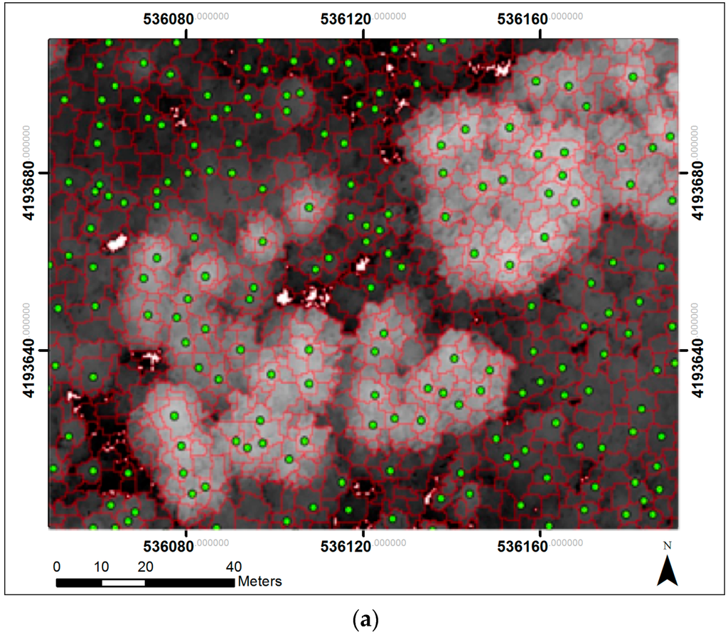
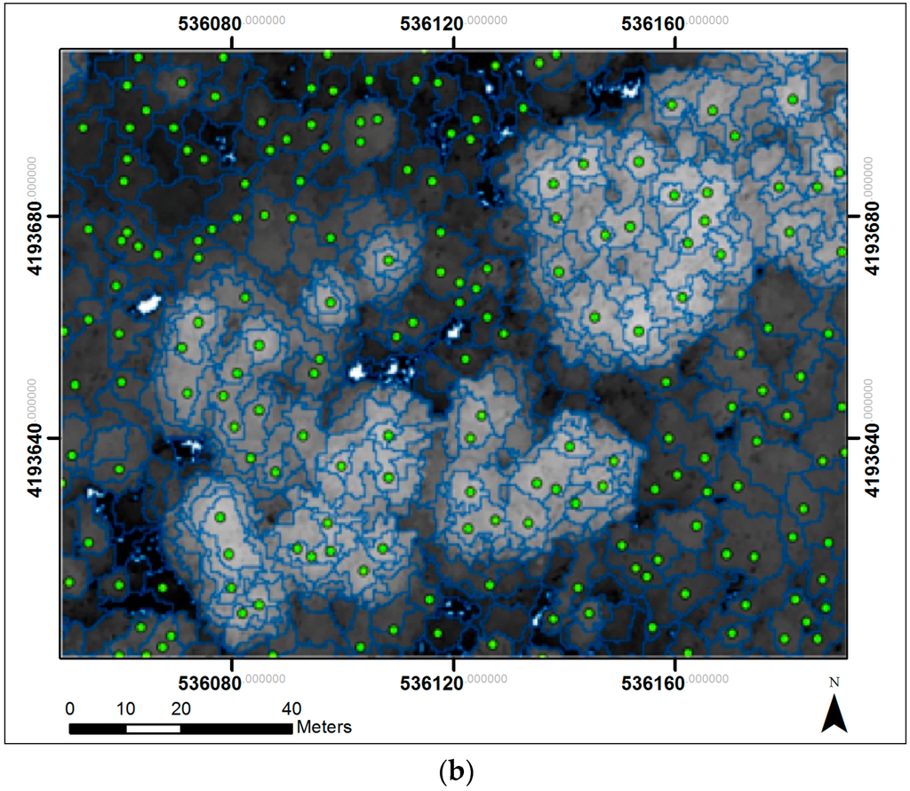
Figure 2.
(a) The small segmentation created by the multi-resolution segmentation in eCognition 9.1 displayed over the canopy height model. Points represent tree centers. Over-segmentation is visible; (b) The large segmentation created by the multi-resolution segmentation shows areas of under-segmentation of merged tree crowns.
The small object segmentation resulted from a scaling parameter of 6, a shape of 0.3 and a compactness of 0.8 using trial and error. These parameters increased the likelihood that a tree stem point was contained within a single object while maintaining a small object size. This approach, however, resulted in an over-segmentation of objects in some areas. The large object segmentation parameters were also determined using trial and error, resulting in a scaling factor of 9, a shape of 0.1 and a compactness of 0.5. Visually, the large object delineation aligned closer to actual tree boundaries of the CHM. In some cases, however, the image was under-segmented in areas where merged tree crowns had similar heights.
2.6. Data Reduction and Feature Selection
To address the problem of high data dimensionality in hyperspectral images, a forward minimum noise fraction (MNF) transform was applied to the mosaicked image to reduce data redundancy and help identify bands containing the most variance. This process creates outputs of uncorrelated bands, which are ranked from highest eigenvalue (with most meaningful bands) to lowest eigenvalue (containing noise-filled bands). Due to the masking of low-lying vegetation, the resulting set of MNF bands was ranked only based on variance within forested areas only. ENVI’s data dimensionality wizard allows for automated estimates of MNF band coherence; however, these estimates are based on default calculations, which risk over- and under-estimation of dimensionality [28]. Alternatively, manual band selection allows for the examination of eigenvalues and visual assessment of MNF band images to determine which are spatially coherent and which contain noise. Based on visual inspection of MNF band images and the consideration of ranked eigenvalues, a total of 27 features (Figure 3) were deemed coherent and informative for use in the final classification (Table 2).
Figure 3.
The first three minimum noise fraction (MNF) band images (a) have high spectral coherence, which helps to distinguish dominant tree species. The final three MNF bands of the 27 selected (b) contain some spectrally-coherent areas (highlighted) within the otherwise noise-filled image.
Table 2.
After the minimum noise fraction transform, 27 bands were selected to be used in the image classifications. The selection of bands was based on the eigenvalues and percentage of data variance, along with visual inspection of each band.
2.7. Sample Data
Stratified random sampling was used to select both training and testing samples for the classification. Single species tree stands were used as strata to reduce potential error when conducting ground truth and to remove the possibility of mixed-species pixels. Field work consisted of navigating to pre-selected random points within stands using GPS and a detailed CHM to confirm the species of the tree at each point. Given the steep terrain and thick vegetation in the study area, samples that could not be checked in the field were confirmed using high resolution reference imagery. From the total samples collected, points were randomly assigned into training and testing samples. Training sample polygons were manually drawn around the training sample points with CHM tree crowns as a guide.
To determine the number of training pixels needed for each class, a common rule suggests multiplying the number of bands used in the classification by ten [46]. Given the object-based approach used in this research, this rule was used as a guideline to select training samples that were then assigned pixel-based and object-based reflectance to understand the influence of training sample size and type on the two classifiers (Table 3). The object-based training sample set was based on the training sample polygons, where the value of the sample equaled the mean spectral reflectance value of the pixels within the polygon. The same training sample polygons were used in the pixel-based training sample set; however, the spectral reflectance of each pixel contained within the polygon was used as a training sample. All samples were proportionally selected for each class.
Table 3.
Training and accuracy assessment samples by class. A total of 806 samples were collected (small training sample set and testing samples). The large training sample set utilized all pixels within the sample polygons as the training samples.
The number of test samples needed for accuracy testing was based on the multinomial distribution for a confidence interval of 90% for the accuracy assessment [47]. Although a confidence interval of 95% would have been preferred, the number of test samples required to attain that level was beyond the scope of this project, especially given the hard to access terrain. Testing samples for each species were also proportionally selected by class size. A total of 663 test samples were determined necessary for a confidence interval of 90%.
2.8. Classification
Eight tree species were used in the classification, including coast redwood (Sequoia sempervirens), Douglas fir (Pseudotsuga menziesii), California bay laurel (Umbellularia californica), coast live oak (Quercus agrifolia), red alder (Alnus rubra), arroyo willow (Salix lasiolepis), eucalyptus (Eucalyptus globulus) and California buckeye (Aesculus californica). These species were selected based on their estimated percent coverage in the study area, as well as visibility in the canopy.
A comparative classification approach was taken to compare the support vector machine to the RBF classifier and the random forest classifier. Additionally, classifications were compared based on the size of the object-oriented segmentation and training samples. The classifier comparisons were divided into a total of 4 classification sets, resulting in eight total classifications, explained below (Table 4).
Table 4.
Classification set based on classifier, training sample size and segmentation size.
All species classifications were performed using eCognition 9.1 Developer software [45]. A grid search to determine optimal parameters for the SVM and random forest classifiers was completed in R-project [48] using the ‘tune’ command in package ‘e1071’ (2014). Calibration samples for parameter tuning were extracted from the training samples of each classification set. The SVM classifier parameters selected include gamma, which controls the smoothness of the hyperplane, and C, which controls the error penalty [23]. The RF parameters include m, the number of features used for training, and N, the number of trees. A framework of the steps for these methods can be found in Figure 4.
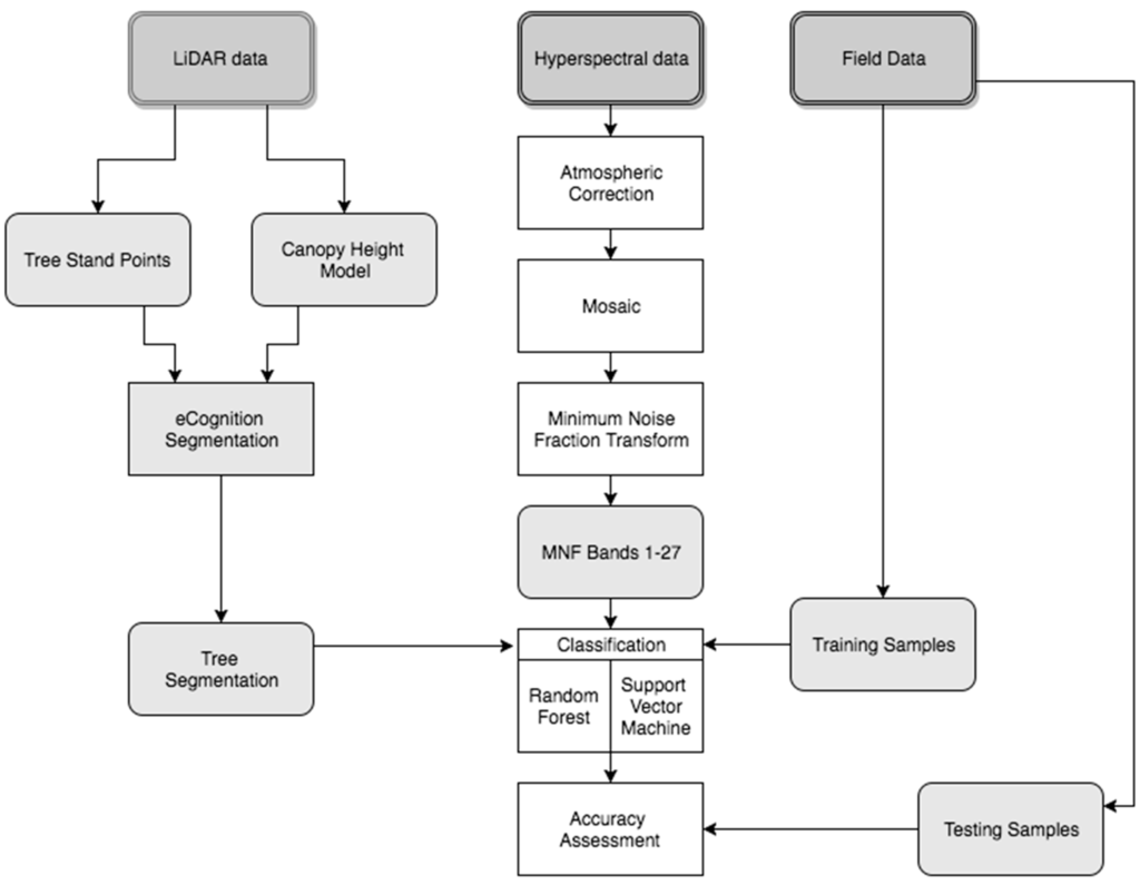
Figure 4.
Framework of the tree species classification using LiDAR, hyperspectral and field data.
2.9. Accuracy Assessment
A visual inspection of each classification was performed to identify areas of potential error and contrast between classifications. The results of the classifications were also assessed according to the confusion matrix based on overall accuracy, user’s accuracy and producer’s accuracy [49].
McNemar’s test has been frequently used for testing the statistical significance of two classifiers [4,20,21,50]. Foody [51] suggests the use of McNemar’s test instead of a z-test in cases where the same test samples are used for each accuracy assessment, resulting in the assumption of independence of samples to not be fulfilled. McNemar’s test [52] measures the error of two proportions that use the same training sample set, where the null hypothesis assumes that the error produced by each classifier is the same [53]. McNemar’s test was used to determine if differences in accuracies between the SVM and RF classifier were statistically significant, as well as any change in performance of the individual classifiers when training and segmentation sizes are adjusted. The confidence interval for statistical testing was 95%.
3. Results
3.1. Overall Classification Results
All four classification sets resulted in overall accuracies above 90% for both the SVM and RF classifiers. The overall accuracies of the first two classification sets showed no statistically-significant difference between classifiers (Table 5). Classification Sets 3 and 4 both resulted in the SVM classifier having a statistically significant advantage over the RF classifier. Classification Set 4, with pixel-based training samples and a large object segmentation size, resulted in the highest accuracies for both classifiers and was considered to be the best scenario.
Table 5.
Statistical significance of the classification sets.
3.2. Best Performance: Classification Set 4
Classification Set 4 resulted in the best performance of both classifiers with overall accuracy for the SVM at 95.02% and RF at 92.91% (Table 6). The difference between classifier overall accuracies was found to be significant.
Table 6.
Confusion matrices for classification Set 4, which resulted in the highest overall accuracies for both classifiers. The top row of classes represents the reference trees, and the left column represents classified trees.
This classification set used pixel-based reflectance training samples to classify the large object segmentation. The SVM parameters were a gamma of 16 and a cost of 0.0156, while the RF parameters had an m of five and N of 2000.
The improvements in overall accuracies were consistent with the visual improvement from other classification sets. With the introduction of pixel-based training samples and a larger segmentation, both classifications showed a visible reduction of misclassifications and improvement in species homogeneity within stands.
As was the case with all other classification sets, visual assessment comparing the SVM and RF classifications consistently found that the SVM classifier resulted in a more homogeneous and generalized classification of species than the random forest classifier (Figure 5). Three areas in the study site tended to have higher instances of misclassification; however, this showed improvement with each classification. The RF classifications consistently misidentified red alder along the right edge of the image, while the SVM classification correctly identified the uniform coverage of Douglas fir (Figure 6). Stands along the western edge of Kent Canyon posed a challenge for the other classification sets, with redwoods misclassified as coast live oak and buckeye. As was true for all other classifications, SVM displayed greater uniformity than RF and resulted in better prediction of classes in this area (Figure 7).
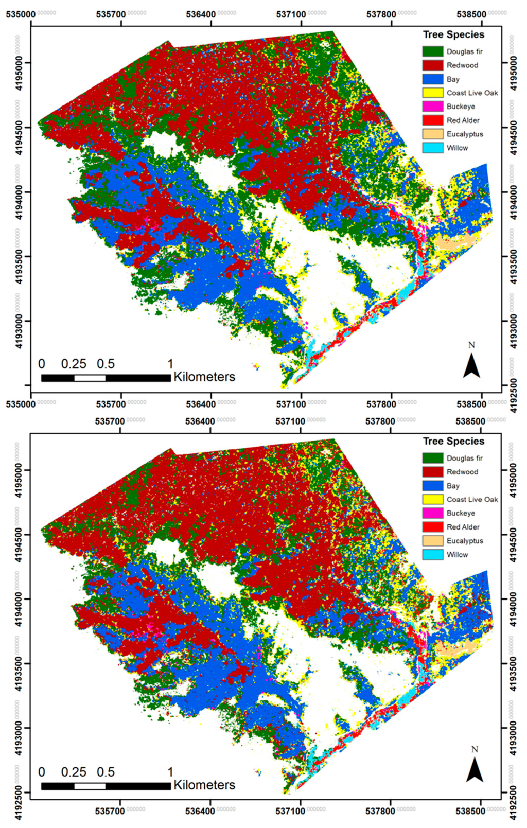
Figure 5.
Classification Set 4. Species classifications of the study area using the support vector machine classifier (top) and random forest classifier (bottom).
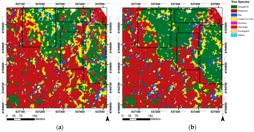
Figure 6.
Classification Set 4 comparison of RF (a) and SVM (b) on the eastern edge of Muir Woods National Monument. The random forest classification (a) shows large groupings of coast live oak (1) and abundant red alder (2), while the support vector machine classification (b) contains less coast live oak and red alder, providing a more accurate representation of the existing tree stands.
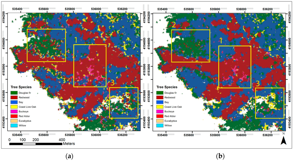
Figure 7.
Classification Set 4 comparison of RF (a) and SVM (b) in Kent Creek Canyon. Both the RF classification (a) and SVM classifications (b) show large areas of misclassified buckeye in the redwood stand (1). The RF classification (a) contains more areas misclassified as redwood and coast live oak (2,3), resulting in more class variation than in the SVM classification (b).
For individual class accuracies, both classifiers resulted in a 57.89% producer’s accuracy for willow, which was consistent with all other classification sets. The RF classifier resulted in the willow user’s accuracy dropping by at least 10% from previous classifications. The RF classifier user’s accuracy for coast live oak remained similar to other classification sets at 62.50%, while the SVM user’s accuracy for coast live oak rose from below 75% in all previous classifications to 90.32%. Aside from coast live oak and willow, both classifiers had producer’s and user’s accuracy above 90% for all other species, showing improvement from other classification sets.
3.3. Individual Classifier Performance
The performances of both the SVM and RF classifiers were assessed individually to determine if the use of pixel-based training samples, segmentation size or both would result in a change of performance. Pixel-based training samples increased the SVM overall accuracy for both the small segmentation and large segmentation with p-values of 0.0258 (Figure 8). With a confidence interval of 95%, the enhanced performance of the SVM classifier can be considered significant. For the RF classifier, improvement in overall accuracy was significant only with the addition of pixel-based training sample size combined with the larger object size. The increase in segmentation object size alone did not improve the SVM or RF classifications with any significance.
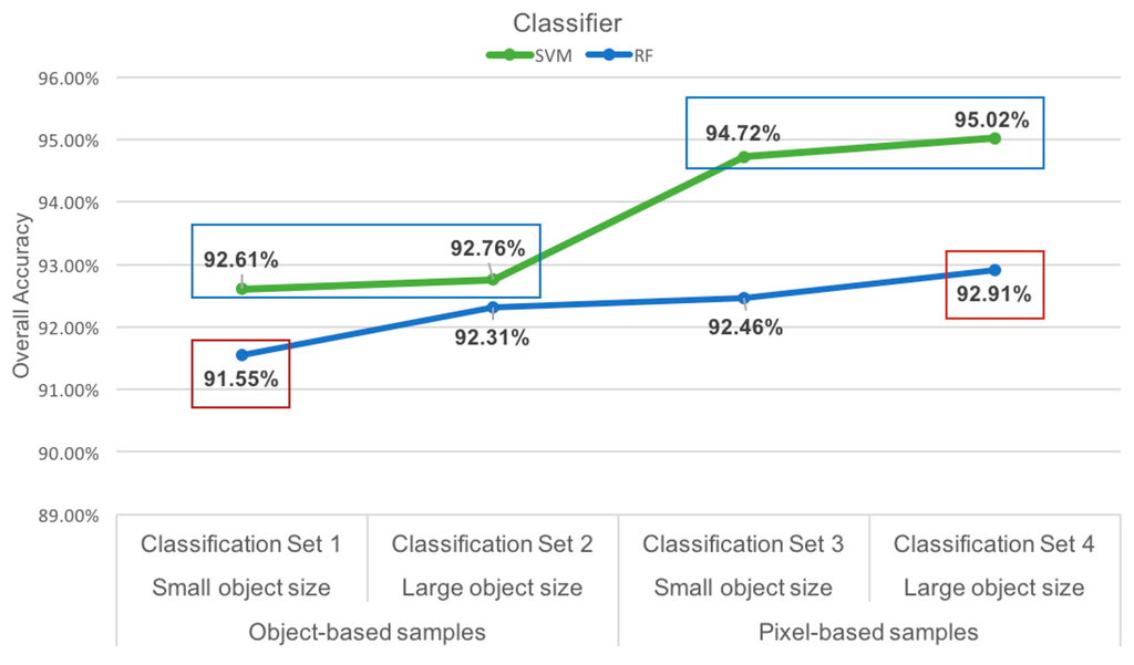
Figure 8.
A graph of classifier performance for each classification approach highlights statistically-significant changes in overall accuracy. The SVM classifier demonstrated significant improvement with the addition of pixel-based training samples. The RF classifier showed significant improvement only with the addition of pixel-based and larger object size.
4. Discussion
In comparing the overall accuracies of the SVM and RF classifier, SVM was determined to have a statistically-significant advantage over RF when the pixel-based reflectance samples were used, irrespective of segmentation size. The most misclassified class for both classifiers was willow, with class accuracies all below 60%. The willow class was misclassified as multiple different species, had the fewest number of training samples and consistently had low class accuracies. Redwood was correctly identified most consistently.
A noticeable trait of both classifiers was the high overall accuracies despite abundant misclassifications found during visual inspection. Duro et al. [54] experienced similar issues with their classification, highlighting that limited testing samples can result in inaccurate classification accuracies. Similarly, Congalton [49] explains that a large quantity of zeroes within the confusion matrix can mean that the test sample size is inadequate or the classification highly successful. Considering the number of zeroes on the confusion matrix for the smaller classes (eucalyptus, willow, coast live oak, etc.), it is quite possible that insufficient test samples were responsible for the high classification accuracies of some species. For this research, the stratified sampling method utilized single species stands to ensure correct sample identification; however, this prevented test samples from being selected near stand boundaries, in mixed forest areas or in inaccessible areas. As a result, the test samples did not represent all areas of the study site, and thus, the accuracy assessment failed to reflect the classifier performance in those areas.
In some cases, an individual species was misclassified as one or two other classes, as was demonstrated by the redwood class commonly being incorrectly classified as bay or Douglas fir. As discussed by Heinzel and Koch [19], misclassification within the same tree types (conifers and broadleaf) occur at a higher rate than they do between tree types. Some broadleaf tree classes (coast live oak, buckeye, red alder) were misclassified as other broadleaf species, likely as a result of similar spectral signatures among the broadleaf species. The fact that Douglas fir and willow were misclassified as many different species of various tree types, however, may suggest a different cause of some misclassifications. Leckie et al. [1] highlight the causes of high spectral variability in old growth forests, which include shadowing, tree health and bidirectional reflectance. Shadowing may best explain the misclassification of Douglas fir as coast live oak throughout the upper portions of the mosaic. Additionally, sun angle and slope can change reflectance values based on date and time of day. Although a normalization was applied to the images before mosaicking, the normalization was likely insufficient for the non-consecutive flight lines. Because training samples from all images were used to train the classifiers, the result was a wider spectral range for some classes. This may have caused spectral overlap, which leads to misclassification of species.
The influence of pixel-based training samples played a significant role in the SVM and RF classifications. The difference between object- and pixel-based training samples can effectively be seen as an increase in sample size. Although the actual number of samples is the same for both sample types, the pixel-based reflectance samples provide additional spectral reflectance values used to train the classifiers. The current literature generally recognizes the support vector machine classifier for its ability to work well with limited training samples [33]. The need for fewer training samples is attributed to the fact that SVM utilizes only the subset of the training samples that defines the location of the SVM hyperplane [23]. Contrary to the majority of the literature, this research suggests that an increase in training size can improve the SVM classifier. Similarly, Zhang and Xie [55] also found that both SVM and RF were sensitive to training size when assessing a complex landscape with high spatial and spectral variability. A possible reason for the greater influence of training sample size in this research could be the complexity and heterogeneity of forest and insufficient object-based samples. Considering the influence of training samples on defining SVM hyperplanes, object-based samples (based on mean pixel values) may fail to capture the high spectral variability within eight tree species in a highly heterogeneous forest as compared to a less complex forest with fewer classes or less spectral overlap of species.
The influence of segmentation size alone had no statistically-significant influence on classification accuracy. Classifications using small segmentations tended to show a greater variety of species within stands, which was likely due to shadowing. Small segmentations that fit entirely within shadowed areas may not have similar spectral properties as sunlit segments of the same class, resulting in a misclassification of shadowed areas. The larger segmentation might include both shadowed and sunlit portions of a tree, resulting in a higher chance of being correctly classified. The result of this artifact is a speckled appearance of species on the small-object classification and a more uniform display of species on the large-object classification.
In the comparison of SVM and RF in forest and land cover classifications, most literature has found that both provide high accuracies with no significant difference between the classifiers [4,53]. Consistent with the literature, both classifiers in this research resulted in high accuracies, which showed no significant difference between methods. However, the addition of pixel-based training samples improved SVM enough to gain a significant advantage. Dalponte et al. [15] found that in a mixed coniferous and broadleaf forest, SVM performed better than RF, likely because RF has been found less able to handle minority classes. Tarabalka et al. [20] also noted with the SVM classifier that classes with small training sample sizes often resulted in low accuracy. The performance of both classifiers on small classes can explain the low class accuracies in Classification Sets 1 and 2, where no difference in classifier performance is found. With the addition of pixel-based samples, the SVM classifier likely improved the handling of the small classes due to the increase in sample size, increasing overall SVM accuracy significantly above RF.
Visually, SVM consistently provided a smooth and less speckled appearance over the RF classifier. While SVM may provide a more visually realistic classification, post-classification processing could minimize visual differences between the classifier outputs [24].
5. Conclusions
An object-based classification of tree species in a complex and heterogeneous forest on challenging topography was performed on a mosaicked hyperspectral image using two commonly-used classifiers. Two variables, training sample type and segmentation size, were adjusted to test classifier performance under these different conditions. Neither classifier outperformed the other statistically when object-based training samples were used, regardless of segmentation size. The SVM classifier accuracy did have a statistical advantage over RF with the addition of pixel-based training samples, likely due to how each classifier handles small classes. Individually, SVM and RF classifiers improved significantly when segmentation size and training sample size increased. In the context of a complex forest with varying class sizes, SVM offers a statistical advantage over RF, assuming sufficient training samples are provided. Additionally, increasing the training sample size may improve the performance of the SVM when small classes are being considered.
Considering the challenging environment of the study area, all classifications successfully resulted in high overall accuracies. The limited accessibility to the study area restricted the number of samples that could be collected, providing additional challenges. Similarly, the sun illumination differences between non-consecutive flight lines, which were enhanced by the steep canyons of the study area, increased opportunities for misclassifications.
Acknowledgments
This work was supported by the National Park Service and California State Parks. We would like to thank the Hyperspectral –LiDAR research lab at University of Victoria, BC, Canada.
Author Contributions
Laurel Ballanti designed the study, performed the experiments, analyzed the data and wrote the paper. Ellen Hines and Leonhard Blesius advised on the study design and edited the paper. Bill Kruse developed data-processing scripts and advised on the methodology.
Conflicts of Interest
The authors declare no conflict of interest.
Abbreviations
The following abbreviations are used in this manuscript:
| DEM | digital elevation model |
| CHM | canopy height model |
| SVM | support vector machine |
| RBF | radial basis function |
| RF | random forest |
| MNF | minimum noise fraction |
References
- Leckie, D.G.; Tinis, S.; Nelson, T.; Burnett, C.; Gougeon, F.A.; Cloney, E.; Paradine, D. Issues in species classification of trees in old growth conifer stands. Can. J. Remote Sens. 2005, 31, 175–190. [Google Scholar] [CrossRef]
- Dalponte, M.; Bruzzone, L.; Gianelle, D. Fusion of hyperspectral and LIDAR remote sensing data for classification of complex forest areas. IEEE Trans. Geosci. Remote Sens. 2008, 46, 1416–1427. [Google Scholar] [CrossRef]
- Peerbhay, K.Y.; Mutanga, O.; Ismail, R. Commercial tree species discrimination using airborne AISA Eagle hyperspectral imagery and partial least squares discriminant analysis (PLS-DA) in KwaZulu–Natal, South Africa. ISPRS J. Photogramm. Remote Sens. 2013, 79, 19–28. [Google Scholar] [CrossRef]
- Ghosh, A.; Fassnacht, F.E.; Joshi, P.K.; Koch, B. A framework for mapping tree species combining hyperspectral and LiDAR data: Role of selected classifiers and sensor across three spatial scales. Int. J. Appl. Earth Obs. Geoinform. 2014, 26, 49–63. [Google Scholar] [CrossRef]
- Franklin, S.E. Remote Sensing for Sustainable Forest Management; CRC Press: Boca Raton, FL, USA, 2001. [Google Scholar]
- Franklin, J. Mapping Species Distributions: Spatial Inference and Prediction; Cambridge University Press: Cambridge, UK, 2010. [Google Scholar]
- Dale, V.; Joyce, L.; McNulty, S.; Neilson, R.; Ayres, M.; Flannigan, M.; Hanson, R.; Irland, L.; Lugo, A.; Peterson, C.; et al. Climate Change and Forest Disturbances. BioScience 2001, 51, 723–734. [Google Scholar] [CrossRef]
- Landgrebe, D. Hyperspectral Image Data Analysis as a High Dimensional Signal Processing Problem. IEEE Signal Process. Mag. 2002, 19, 17–28. [Google Scholar] [CrossRef]
- Gislason, P.O.; Benediktsson, J.A.; Sveinsson, J.R. Random forests for land cover classification. Pattern Recognit. Lett. 2006, 27, 294–300. [Google Scholar] [CrossRef]
- Van Aardt, J.A.N.; Wynne, R.H. Examining pine spectral separability using hyperspectral data from an airborne sensor: An extension of field-based results. Int. J. Remote Sens. 2007, 28, 431–436. [Google Scholar] [CrossRef]
- Martin, M.E.; Newman, S.D.; Aber, J.D.; Congalton, R.G. Determining forest species composition using high spectral resolution remote sensing data. Remote Sens. Environ. 1998, 65, 249–254. [Google Scholar] [CrossRef]
- Clark, M.L.; Roberts, D.A.; Clark, D.B. Hyperspectral discrimination of tropical rain forest tree species at leaf to crown scales. Remote Sens. Environ. 2005, 96, 375–398. [Google Scholar] [CrossRef]
- Akar, Ö.; Güngör, O. Classification of multispectral images using Random Forest algorithm. J. Geod. Geoinform. 2012, 1, 105–112. [Google Scholar] [CrossRef]
- Holmgren, J.; Persson, A.; Söderman, U. Species identification of individual trees by combining high resolution LiDAR data with multi-spectral images. Int. J. Remote Sens. 2008, 29, 1537–1552. [Google Scholar] [CrossRef]
- Dalponte, M.; Bruzzone, L.; Gianelle, D. Tree species classification in the Southern Alps based on the fusion of very high geometrical resolution multispectral/hyperspectral images and LiDAR data. Remote Sens. Environ. 2012, 123, 258–270. [Google Scholar] [CrossRef]
- Key, T.; Warner, T.A.; McGraw, J.B.; Fajvan, M.A. A comparison of multispectral and multitemporal information in high spatial resolution imagery for classification of individual tree species in a temperate hardwood forest. Remote Sens. Environ. 2001, 75, 100–112. [Google Scholar] [CrossRef]
- Franklin, S.E.; Hall, R.J.; Moskal, L.M.; Maudie, A.J.; Lavigne, M.B. Incorporating texture into classification of forest species composition from airborne multispectral images. Int. J. Remote Sens. 2000, 21, 61–79. [Google Scholar] [CrossRef]
- Shippert, P. Why use hyperspectral imagery? Photogramm. Eng. Remote Sens. 2004, 70, 377–396. [Google Scholar]
- Heinzel, J.; Koch, B. Investigating multiple data sources for tree species classification in temperate forest and use for single tree delineation. Int. J. Appl. Earth Obs. Geoinform. 2012, 18, 101–110. [Google Scholar] [CrossRef]
- Tarabalka, Y.; Chanussot, J.; Benediktsson, J.A. Segmentation and classification of hyperspectral images using watershed transformation. Pattern Recognit. 2010, 43, 2367–2379. [Google Scholar] [CrossRef]
- Jones, T.G.; Coops, N.C.; Sharma, T. Assessing the utility of airborne hyperspectral and LiDAR data for species distribution mapping in the coastal Pacific Northwest, Canada. Remote Sens. Environ. 2010, 114, 2841–2852. [Google Scholar] [CrossRef]
- Hughes, G.F. On the mean accuracy of statistical pattern recognizers. IEEE Trans. Inform. Theory 1968, 14, 55–63. [Google Scholar] [CrossRef]
- Melgani, F.; Bruzzone, L. Classification of hyperspectral remote sensing images with support vector machines. IEEE Trans. Geosci. Remote Sens. 2004, 42, 1778–1790. [Google Scholar] [CrossRef]
- Rojas, M.; Dópido, I.; Plaza, A.; Gamba, P. Comparison of support vector machine-based processing chains for hyperspectral image classification. Proc. SPIE 2010. [Google Scholar] [CrossRef]
- Voss, M.; Sugumaran, R. Seasonal effect on tree species classification in an urban environment using hyperspectral data, LiDAR, and an object-oriented approach. Sensors 2008, 8, 3020–3036. [Google Scholar] [CrossRef]
- Buddenbaum, H.; Schlerf, M.; Hill, J. Classification of coniferous tree species and age classes using hyperspectral data and geostatistical methods. Int. J. Remote Sens. 2005, 26, 5453–5465. [Google Scholar] [CrossRef]
- Denghui, Z.; Le, Y. Support vector machine based classification for hyperspectral remote sensing images after minimum noise fraction rotation transformation. In Proceedings of the 2011 International Conference on Internet Computing & Information Services (ICICIS), Hong Kong, China, 17–18 September 2011.
- Exelis Visual Information Solutions. ENVI Help; Exelis Visual Information Solutions: Boulder, CO, USA, 2013. [Google Scholar]
- Xiao, Q.; Ustin, S.L.; McPherson, E.G. Using AVIRIS data and multiple-masking techniques to map urban forest tree species. Int. J. Remote Sens. 2004, 25, 5637–5654. [Google Scholar] [CrossRef]
- Dalponte, M.; Ørka, H.O.; Ene, L.T.; Gobakken, T.; Naesset, E. Tree crown delineation and tree species classification in boreal forests using hyperspectral and ALS data. Remote Sens. Environ. 2014, 140, 306–317. [Google Scholar] [CrossRef]
- Alonzo, M.; Bookhagen, B.; Roberts, D.A. Urban tree species mapping using hyperspectral and lidar data fusion. Remote Sens. Environ. 2014, 148, 70–83. [Google Scholar] [CrossRef]
- MacLean, M.G.; Congalton, R. Map accuracy assessment issues when using an object-oriented approach. In Proceedings of the American Society for Photogrammetry and Remote Sensing 2012 Annual Conference, Sacramento, CA, USA, 19–23 March 2012.
- Mountrakis, G.; Im, J.; Ogole, C. Support vector machines in remote sensing: A review. ISPRS J. Photogramm. Remote Sens. 2011, 66, 247–259. [Google Scholar] [CrossRef]
- Breiman, L. Random forests. Mach. Learn. 2001, 45, 5–32. [Google Scholar] [CrossRef]
- Cutler, D.R.; Edwards, T.C., Jr.; Beard, K.H.; Cutler, A.; Hess, K.T.; Gibson, J.; Lawler, J.J. Random forests for classification in ecology. Ecology 2007, 88, 2783–2792. [Google Scholar] [CrossRef] [PubMed]
- Schoenherr, A.A. A Natural History of California; University of California Press: Berkeley, CA, USA, 1992. [Google Scholar]
- National Parks Conservation Association. State of the Parks, Muir Woods National Monument: A Resource Assessment. 2011. Available online: http://www.npca.org/about-us/center-for-parkresearch/stateoftheparks/muir_woods/MuirWoods.pdf (accessed on 22 October 2014).
- National Park Service. Annual Park Recreation Visitation (1904—Last Calendar Year) Muir Woods NM (MUWO) Reports. 2014. Available online: https://irma.nps.gov/Stats/Reports/Park/MUWO (accessed on 6 October 2015). [Google Scholar]
- National Park Service. Muir Woods: 100th Anniversary 2008; 2008. Available online: http://www.nps.gov/muwo/upload/unigrid_muwo.pdf (accessed on 22 October 2014).
- Ellen, H. Final Report: Golden Gate LiDAR Project; San Francisco State University: San Francisco, CA, USA, 2011. [Google Scholar]
- Stephen, R. GGLP SFSU Hyperspectral Processing Report; University of Victoria- Hyperspectral—LiDAR Research Laboratory: Victoria, BC, Canada, 2013. [Google Scholar]
- QCoherent. LP360, Version 2013. Available online: http://www.qcoherent.com/ (accessed on 30 April 2013).
- GRASS Development Team. Geographic Resources Analysis Support System (GRASS) Software, Version 6.4.4. Available online: http://grass.osgeo.org (accessed on 3 May 2015).
- Trimble. eCognition Developer, Version 9.1. Available online: http://www.ecognition.com (accessed on 12 May 2015).
- Trimble. eCognition: User Guide 9.1; Trimble: Munich, Germany, 2015. [Google Scholar]
- McCoy, R.M. Field Methods in Remote Sensing; Guilford Press: New York City, NY, USA, 2005. [Google Scholar]
- Congalton, R.G.; Green, K. Assessing the Accuracy of Remotely Sensed Data: Principles and Practices; CRC Press: Boca Raton, FL, USA, 2008. [Google Scholar]
- R Core Team. R: A Language and Environment for Statistical Computing; R Foundation for Statistical Computing: Vienna, Austria, 2015; Available online: http://www.R-project.org/ (accessed on 10 June 2015).
- Congalton, R.G. A review of assessing the accuracy of classifications of remotely sensed data. Remote Sens. Environ. 1991, 37, 35–46. [Google Scholar] [CrossRef]
- Pal, M.; Foody, G.M. Feature selection for classification of hyperspectral data by SVM. IEEE Trans. Geosci. Remote Sens. 2010, 48, 2297–2307. [Google Scholar] [CrossRef]
- Foody, G. Thematic map comparison: Evaluating the statistical significance differences in classification accuracy. Photogramm. Eng. Remote Sens. 2004, 70, 627–633. [Google Scholar] [CrossRef]
- Everitt, B.S. The Analysis of Contingency Tables; Chapman and Hall: London, UK, 1977. [Google Scholar]
- Dietterich, T. Approximate statistical tests for comparing supervised classification learning algorithms. Neural Comput. 1998, 10, 1895–1923. [Google Scholar] [CrossRef] [PubMed]
- Duro, D.C.; Franklin, S.E.; Dubé, M.G. A comparison of pixel-based and object-based image analysis with selected machine learning algorithms for the classification of agricultural landscapes using SPOT-5 HRG imagery. Remote Sens. Environ. 2012, 118, 259–272. [Google Scholar] [CrossRef]
- Zhang, C.; Xie, Z. Object-based vegetation mapping in the Kissimmee River watershed using HyMap data and machine learning techniques. Wetlands 2013, 33, 233–244. [Google Scholar] [CrossRef]
© 2016 by the authors; licensee MDPI, Basel, Switzerland. This article is an open access article distributed under the terms and conditions of the Creative Commons Attribution (CC-BY) license (http://creativecommons.org/licenses/by/4.0/).