Article

Automatic Forest Mapping at Individual Tree Levels from Terrestrial Laser Scanning Point Clouds with a Hierarchical Minimum Cut Method

1
State Key Laboratory of Information Engineering in Surveying, Mapping and Remote Sensing, Wuhan University, Wuhan 430079, China
2
Collaborative Innovation Center of Geospatial Technology, Wuhan University, Wuhan 430079, China
*
Authors to whom correspondence should be addressed.
Remote Sens. 2016, 8(5), 372; https://doi.org/10.3390/rs8050372
Submission received: 4 January 2016 / Revised: 12 April 2016 / Accepted: 25 April 2016 / Published: 3 May 2016

Abstract

:
Laser scanning technology plays an important role in forest inventory, as it enables accurate 3D information capturing in a fast and environmentally-friendly manner. The goal of this study is to develop methods for detecting and discriminating individual trees from TLS point clouds of five plots in a boreal coniferous forest. The proposed hierarchical minimum cut method adopts the detected trunk points that are recognized according to pole like shape segmentation as foreground seed points and other points as background seed points, respectively. It constructs the undirected weighted graph of the foreground and background seed points to deduce a cost function for tree crown point segmentation with the decreasing ranking of tree trunk heights. The intermediate results lead to global optimization segmentation of individual trees in a hierarchical order. Finally, the structure metrics of the detected individual trees are calculated and checked with field observations. Plots with different attributes were selected to verify the proposed method, and the experimental studies show that the proposed method is efficient and robust for extracting individual trees from TLS point clouds in terms of the recall of 90.42%.

Graphical Abstract

1. Introduction

Forests are the dominant terrestrial ecosystem on Earth and provide all kinds of services to humans. In recent years, light detection and ranging (LiDAR) has become an increasingly popular tool for forest monitoring and vegetation mapping tasks for its capacity of obtaining the spatial distribution of surface characteristics with dense point clouds [1,2,3]. Extensive studies have been investigated to estimate forest attributes from point clouds, including tree locations [4], heights [5,6,7], DBH [8], stem curves [9], crown widths [5,10,11,12], crown base heights [13,14], wood volumes [15,16] and biomass [17,18,19,20]. Moreover, the improvement in LiDAR technology of higher pulse rates and the increasing LiDAR posting densities have provided better opportunities for obtaining forest data at a fine scale, and the forest inventory has transferred from an average forest stand scale to the individual tree level [21]. This is also encouraged by the fact that the detailed structures of trees are needed in many forest application, such as ecology, wildlife or biodiversity [10]. However, the fine-scale forest inventory poses great challenges for data processing. In fact, for the delineation and discrimination of single trees in the forest, the difficulties are predominantly the variability of tree crown structures and connected and clumped crowns in dense and complex forest environments. Compared to the individual trunk recognition, the connected crowns and crowns in the multi-layer canopy are more challenging to delineate.
Much of the research into the structure metrics of forests focus on airborne LiDAR point clouds. These studies provide stand or tree characteristics at large scale, but with the cost of missing details at the branch level [22]. In general, the delineation of individual trees in airborne LiDAR point clouds is performed by segmenting canopy height models (CHM) with region growing or watershed solutions [23,24]. The local maxima is used to position treetops. The above solutions perform well in structurally-homogeneous plantations, single-species-dominated stands and forests with widely-spaced trees [11]. However, positioning treetops with the local maxima may lead to commission errors because of complicated tree crown shapes and noisy LiDAR point clouds. For example, the non-treetop local maxima may incorrectly be classified as treetops [5,25].
As a complement to airborne LiDAR, terrestrial laser scanning (TLS) and mobile laser scanning (MLS) enable one to capture the underneath canopy structure and make forest mapping at the detailed individual tree structure level available [26]. Many researchers have worked on stem mapping and stem characteristic (DBH, stem curves) estimation; however, a few studies have focused on individual tree or tree crown delineation from TLS or MLS point clouds. For example, Liang et al. [27] present a fully-automatic stem mapping algorithm by calculating the spatial distribution properties of laser points. Then, the stem model is built up of a series of cylinders, and the location of the stem is estimated by the model. Arachchige [28] utilizes geometric features (such as the principal direction and the shape of point subsets) to extract stems from high density MLS point clouds in urban environments. Xia et al. [29] identify stem points with a two-scale classification method and then use a simple stem curve model to merge stem points. Some attempts have also been made to segment single trees and to delineate crowns in ground-based LiDAR point clouds. Srinivasan et al. [7] establish a regression relationship between field measured crown widths and DBH and apply it in the forest in order to obtain crown information. Lalonde et al. [30] used a Gaussian mixture model and the expectation maximization (EM) algorithm to train the system to recognize and group points belonging to stems, ground and foliage. Rutzinger et al. [31] used the vertical density profile model to separate trees from the ground vegetation. Olofsson et al. [32] classify and measure tree stems and canopies using the Hough transformation and the random sample consensus (RANSAC) algorithm in forest stands with single dominating tree species. These algorithms fit the pre-defined geometrical models to the point clouds with pre-defined parameters and have a risk of missing trees that have shapes different from the pre-defined models [33].
The reported methods of single tree segmentation or crown delineation from TLS or MLS point clouds show relatively satisfactory performance. However, they are performed under a certain type of simplified model and assumptions regarding the structure of tree crowns and their layout in the forest and have a tendency to overlook the young and little trees in the lower canopy layer. Accurate individual tree crown segmentation using TLS data in a forest setting is still a challenging issue, particularly for the connected and clumped crowns, as well as crowns in a multi-layer canopy.
This paper proposes a novel approach for extracting individual trees from TLS point clouds. The individual trunks and tree locations are identified and acquired firstly, then a hierarchical minimum cut operator is proposed to delineate the crown corresponding to each trunk from the point clouds. The contributions of the proposed method are listed as follows:
  • precisely segment the crown points to the corresponding tree trunks in boreal coniferous forest plots with heterogeneous structures;
  • implement a hierarchical strategy to isolate single trees from point clouds reliably; and
  • estimate structure metrics at the individual tree level.
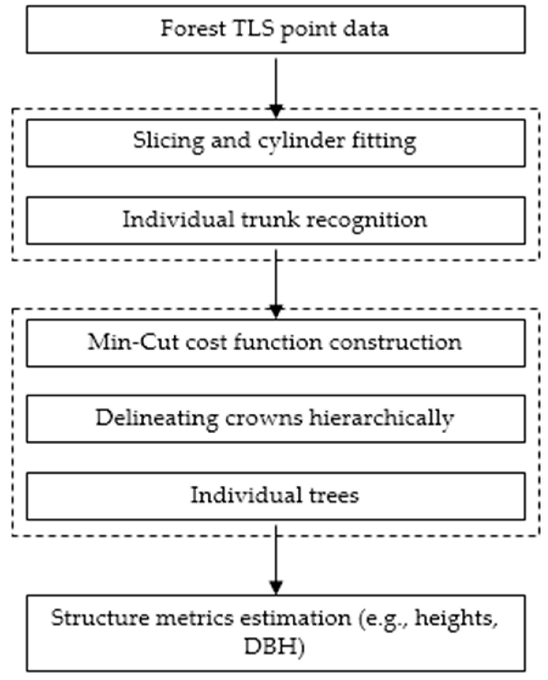
This paper is structured as follows: In Section 2, we present a step-wise description of the proposed method, and in Section 3, the proposed method was tested with the TLS point clouds in different forest settings. Following the experiments, we validate and discuss the tree extraction results. Finally, conclusions are drawn in Section 4.

2. Methodology

The proposed method encompasses three key steps: locating candidate trees, isolating an individual tree and estimating structure metrics at the individual tree level (e.g., tree locations, DBH, heights and stem curves). Firstly, trunks are detected by analyzing the geometric shape characteristics; the intersections between trunks and ground are marked as the tree locations. Secondly, individual trees are isolated by a hierarchical minimum cut approach. For each tree discrimination, the candidate tree trunk points and other tree trunk points are marked as foreground and background seed points, respectively. The hierarchical operator results in tree detection in order from the highest tree to the lowest one. Finally, the structure metrics of the extracted individual trees are calculated according to the single tree point clouds and evaluated with field measurements. The workflow is implemented on several different boreal coniferous forest environment datasets, and the results are evaluated and analyzed. Five forest datasets with different tree densities are utilized to test the method, and it proves successful as a promising solution to extract individual tree from TLS point clouds. The framework of the proposed method is summarized in Figure 1. The detailed description will be given in the following subsections.

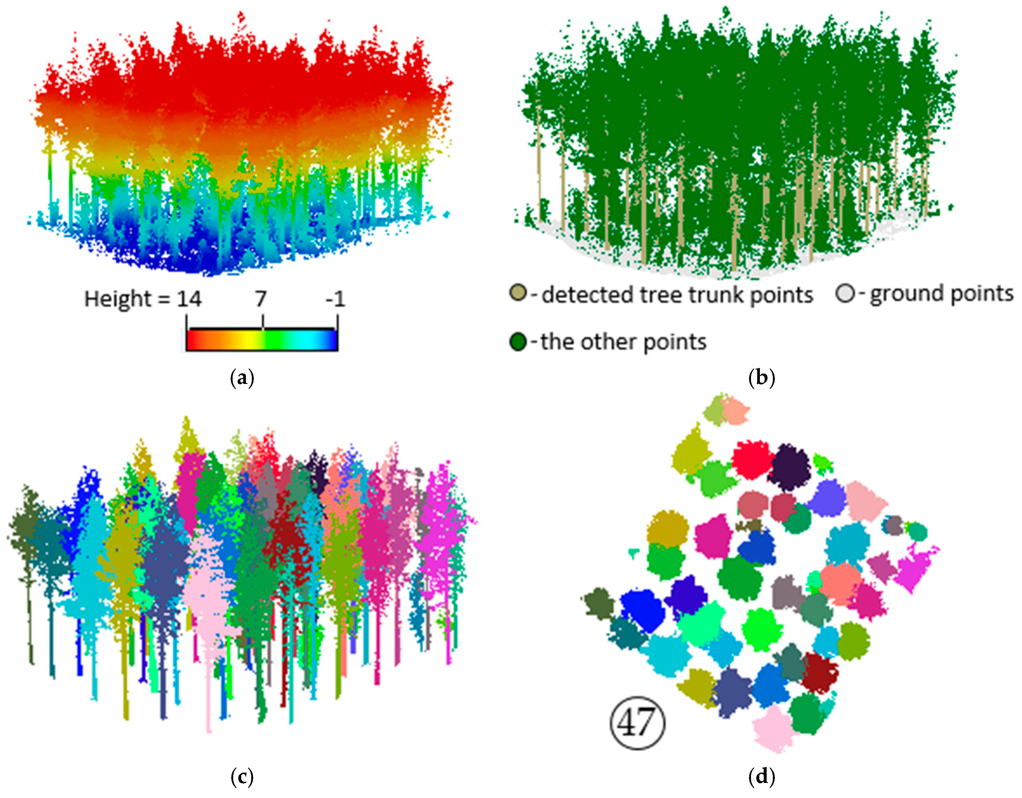
2.1. Localization of Candidate Trees

To discriminate the point clouds of candidate trees from TLS point clouds, the ground points are firstly removed using the method of [34]. The remaining points are regarded as tree points, including trunk points, crown points and other points. Once the trunk points are recognized, the tree locations can thus be calculated according to the intersections between the ground and the corresponding trunk points, and the corresponding tree crown points of each tree trunk are further isolated.
To differentiate tree trunk points from point clouds, first the point clouds are cut with a series of horizontal planes with equal intervals along the vertical direction, resulting in many slices perpendicular to the vertical direction. The thickness of the slice Hslice can be defined according to the point density. Then, the points in each slice are clustered according to a Euclidean clustering algorithm [29]. Hence, the point clouds in all slices are segmented as a set of segments, as illustrated in Figure 2.
Compared to the shapes of other objects, tree trunks show distinguishable shape characteristics of pole-like objects. Hence, the segments in each slice are fitted by a cylinder with a limited radius ranging to find the pole-like segments in the vertical direction. As far as a standard cylinder in the vertical direction is concerned, it can be written as:
| | ( P - Q ) × a | | - r c = 0
r c _ m i n r c r c _ m a x
where P    =    { x p , y p , z p } is a point on the cylinder surface, Q    =    { x q , y q , z q } is a point on the axis, a = {ax, ay, az} is the direction of the cylinder axis with a unit length and parallel to the Z axis (0.0, 0.0, 1.0) and rc is the radius of the cylinder, ranging from r c _ m i n to r c _ m a x .
If a segment unit satisfies the above conditions, it is marked as a segment of trunks. The marked segments are then clustered if the segments distribute along one vertical direction, resulting in many large segments that are regarded as tree trunks. Finally, the intersection points between trunks and ground points are calculated as the location of each tree trunk, as illustrated in Figure 3.

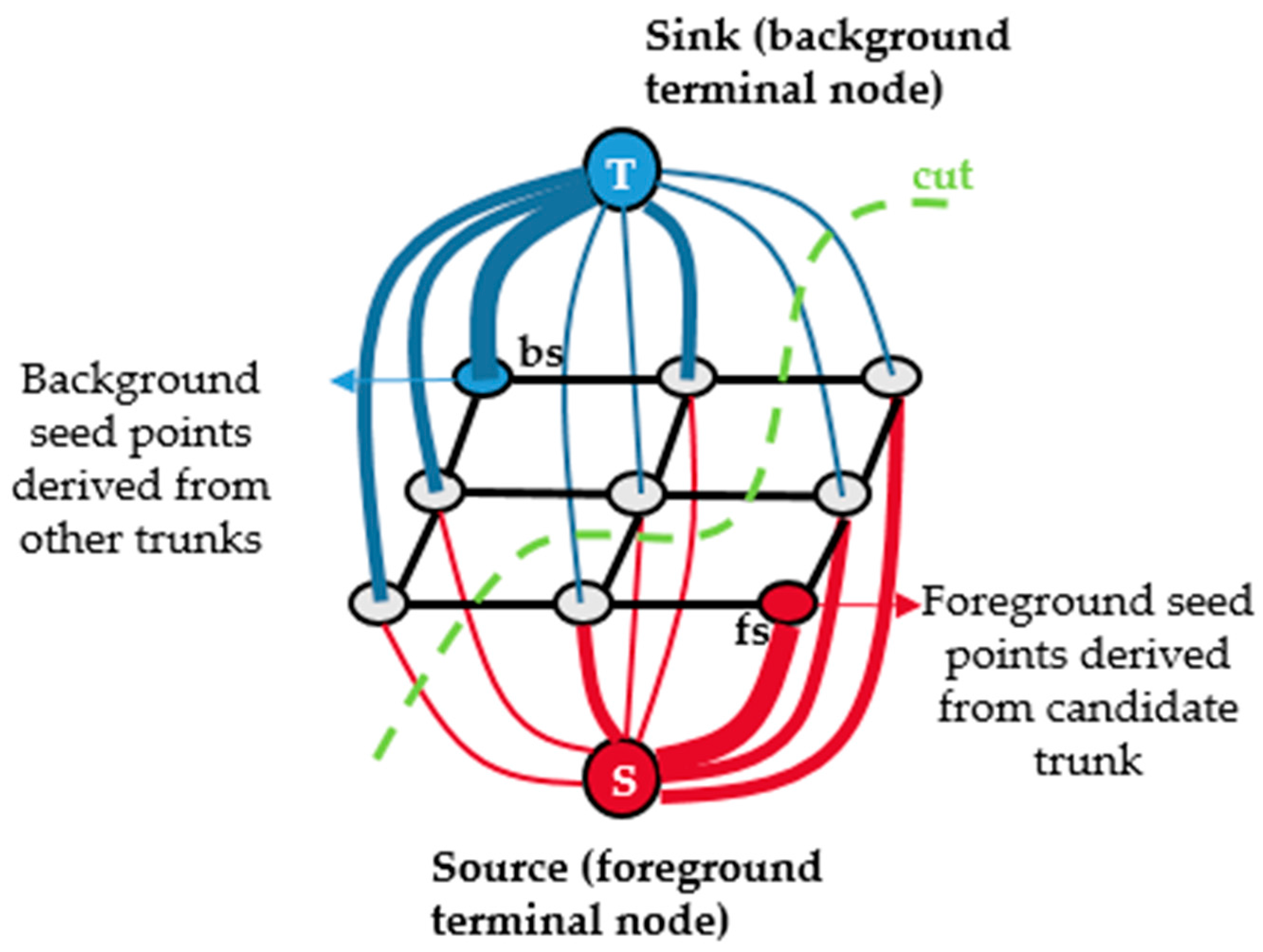
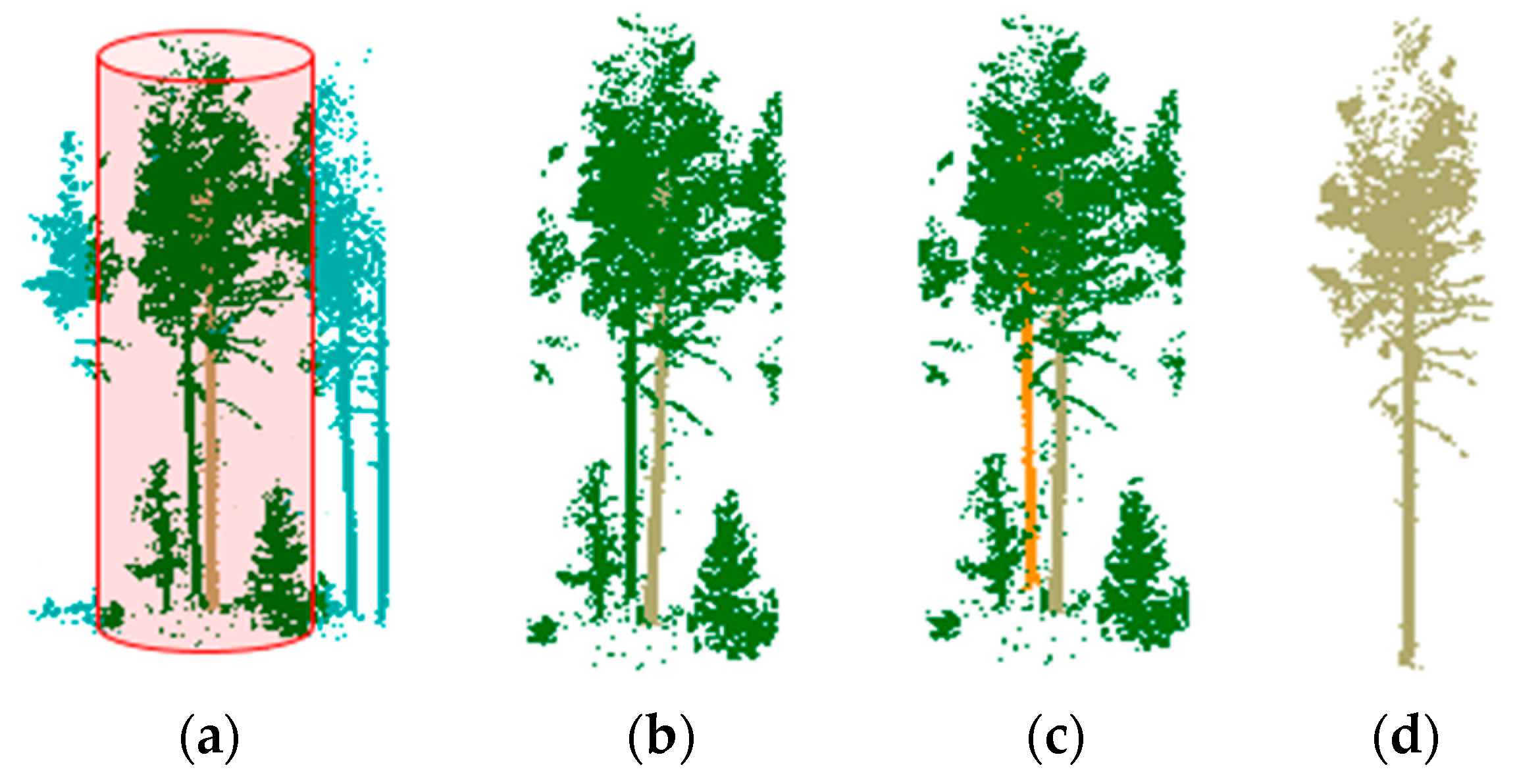
2.2. Isolating Tree Crown Points with the Hierarchical Minimum Cut Operator

Once the tree trunks points are marked, most of the remaining points are regarded as tree crown points. As the tree crowns are often clumped and connected together, it is necessary to correctly isolate the tree crown points corresponding to each trunk, which is the foundation to calculate typical structure metrics (e.g., heights) of an individual tree. To extract each tree crown points, we implemented a hierarchical minimum cut operator by extending the minimum cut algorithm [35,36,37]. The hierarchical minimum cut operator aims to iteratively extract the tree crown points corresponding to each tree trunk in the rank of decreasing trunk height, according to the principles of the minimum cut method. The minimum cut method can achieve the global optimal solution under the minimum cost function. As far as one detected tree trunk is concerned, the hierarchical minimum cut operator aims to segment the points as either foreground (belonging to the candidate tree) or background (not belonging to the candidate tree) by constructing a cost function to achieve the globally optimal segmentation results.
To reduce the time costs of the hierarchical minimum cut operator, only those points that are neighboring the candidate tree trunk are used to calculate the cost function and to join the segmentation of the candidate tree crown points. The cost function is constructed according to the undirected weighted graph of the neighboring points of each tree trunk. The neighboring points of each tree trunk are determined using a cylindrical buffering zone. The cylindrical buffering zone is calculated according to the center of the candidate tree location and a horizontal distance Rb. The points locating in the cylindrical buffering zone are regarded as the input point cloud of the candidate tree segmentation, as illustrated in Figure 5a. The radius of the cylindrical buffering zone Rb is calculated by:
R b = k d t
where k is a constant value and dt is the planar distance between the candidate tree location and its nearest tree location. The constant value k is greater than 1.
Once the input points of one candidate tree are searched, these points will join in the cost function construction to delineate the candidate tree points. Additionally, the optimal segmentation solution is obtained by minimizing the cost function. We use a graph-cut solver to minimize the cost function [38]. Thus, an undirected weighted graph G (V, E, W) of the input points is constructed. In the undirected weighted graph G (V, E, W), V and E are the nodes and edges in the graph, and W is the weight of each edge. The graph G (V, E, W) contains two kind of nodes: ordinary nodes and specially designated nodes. In Figure 4, the nine small dots are ordinary nodes corresponding to the cloud point, and the two bigger ones are specially designated terminal nodes S (source) and T (sink) that represent “foreground” and “background” labels, respectively. The “bs” node (small blue dot in Figure 4) and “fs” node (small red dot Figure 4) are seed points (cloud points whose labels are known before segmentation). The edges can be divided into two groups, n-links and t-links. The black solid lines that connect neighboring cloud points are n-links. The blue and red solid lines that associate ordinary nodes with source and sink nodes are called t-links. Each cloud point is connected to both the source and the sink with t-link edges.
Each edge in the graph was assigned with a non-negative weight, which was also called the cost of the edge. The cost of each edge is reflected by the edge’s thickness. We can see that the t-links that connect a seed point with its corresponding label have a thicker edge. Here, the detected trunk points serve as seed points in the candidate tree segmentation. More specifically, the trunk points of the candidate tree are marked as foreground seed points, and other trunk points in the input cloud are marked as background seed points.
The green dashed line is a cut that divides the graph into two independent parts, foreground and background. A cut is a subset of edges C ∈ E, such that the terminals S and T become completely separated on G (V, E, W). Therefore, any cut corresponds to some binary label vector that partitions an input cloud into “foreground” and “background” segments. The cost of a cut is defined as the sum of the costs of severed edges. The cut that has the minimum cost is minimum cut C min :
C min =    a r g m i n e c W e
It is proven that the minimum cut corresponds to the minimum cost function. Therefore, the segmentation result is controlled by the weights of edges. More specifically, the minimum cost function is written by:
a r g m i n C ( A )    =    p P R p ( A p )    + { p , q } N B p , q δ A p A q
δ A p A q = { 1 i f A p A q 0 i f A p = A q
where A is a binary vector whose component A p specifies the label of each cloud point p. R p ( A p ) denotes the regional term, representing the cost of the t-link for assigning cloud point p to label A p . B p , q refers to the boundary term, representing the pairwise cost of the n-link for connecting neighbor cloud points. The boundary term B p , q is located at the segmentation boundary and ensures the smoothness of the segmentation, while the regional term R p ( A p ) represents the regional properties of segments. As mentioned above, the segmentation result is controlled by the weights of edges. The detailed description of the weights will be given below.
The boundary term is interpreted as a penalty for a discontinuity between neighbor cloud points p and q. Each cloud point is connected with its k-nearest neighbors, and the corresponding cost is calculated by:
B p , q = e x p ( - ( d i / σ ) 2 )
where di is the distance between the neighboring input points p and q and σ is the average span of the points. The larger distance between p and q indicates weaker linking between them.
The regional term indicates the foreground penalty and the background penalty for assigning points to S and T, respectively. The foreground penalty W e i g h t ( p , S ) is specified as a constant value, and the background penalty W e i g h t ( p , T ) is calculated by:
W e i g h t ( p , T ) =    d i s 2 D r a d i u s
where r a d i u s roughly considered as the foreground horizontal range. The planar distance between the candidate tree location and its nearest tree location dt serves as the r a d i u s . d i s 2 D is the planar distance between point clouds and the candidate tree location. Therefore,
R p ( A p ) = { c o n s t a n t   v a l u e i f   A p = f o r e g r o u n d d i s 2 D r a d i u s i f   A P = b a c k g r o u n d
According to Equation (8), the farther a point is from the candidate tree location, the bigger the background penalty of the cloud point will be and the thicker the corresponding edge will be. Thus, cloud points far from a candidate tree location are encouraged to be labeled as “background”. Moreover, the horizontal distance to the candidate tree location is relative to the r a d i u s . Specifically, the minimum r a d i u s is specified empirically as 1 m, indicating that the minimum foreground horizontal range is 1 m.
When the hierarchical minimum cut operator segments the input points of one candidate tree, the tree trunk points of the candidate tree serve as the foreground seed points, and the other neighboring trunk points serve as the background seed points. As shown in Figure 5c, the foreground and background seed points are marked in brown and orange, respectively. Finally, the candidate tree points are delineated by the minimum cost function strategy to achieve the global optimal segmentation (Figure 5d).
In order to reduce the uncertainties of tree crown point segmentation in the area with dense trees, the trunks are ranked in decreasing order of lengths. The hierarchical minimum cut operator segments the tree crown points according to the ranked tree trunks one by one. Once the tree crown points of one candidate tree are segmented, the tree crown points and the corresponding tree trunk points are removed from the point clouds. Hence, the hierarchical minimum cut operator segments the buffer zone points of one candidate tree each time instead of the whole point cloud. Moreover, the detected tree crown points are removed from the point cloud before the next segmentation, thus reducing the uncertainties of adjacent tree crown point segmentation.

2.3. Estimating Structure Metrics at the Tree Level

Once the tree crown points of each tree trunk are isolated, the points of individual trees are determined. Hence, the structure metrics are calculated according to the points of individual trees. The intersection between each tree trunk and ground level is calculated as the location of each tree. The height of each tree is calculated by:
t r e e _ h e i g h t = Z ( P t o p - Z ( P g r o u n d ) )
where Z ( P t o p ) is the maximum elevation of all individual tree points and Z ( P g r o u n d ) is the elevation of the individual tree location at the ground level.
The DBH of each tree is measured according to the diameter of the fitted cylinder of the corresponding tree trunk above ground 1.2 to 1.4 m. The stem curves of tree trunks are calculated at different heights, ranking from 0.65 m to the tree trunk height with a certain height interval.

3. Results and Analysis

3.1. Data Description

The proposed method was tested with five boreal coniferous forest plots with heterogeneous structures, and the point clouds were captured by the Leica HDS6100 terrestrial laser scanner in summer 2014. The five datasets are provided by Finnish Geospatial Research Institute (FGI) for project “Benchmarking on Terrestrial Laser Scanning for Forestry Applications”. This project was launched in order to understand the optimum data processing technique for future automated plot inventories. Test plots are located in a boreal coniferous forest in Evo, Finland (61.19°N, 25.11°E). Each plot has a fixed size, 32-by-32 m. These forest plots vary in species, growth stages and management activities. The main tree species are Scots pine, Norway spruce and silver and downy birches. The details of the datasets are listed in Table 1. Reference data are measured by FGI in the field. All trunks with DBH greater than 5 cm are included in the reference measurements. All of the five test datasets have a reference location. Only Plot 1 has references for tree height and DBH.

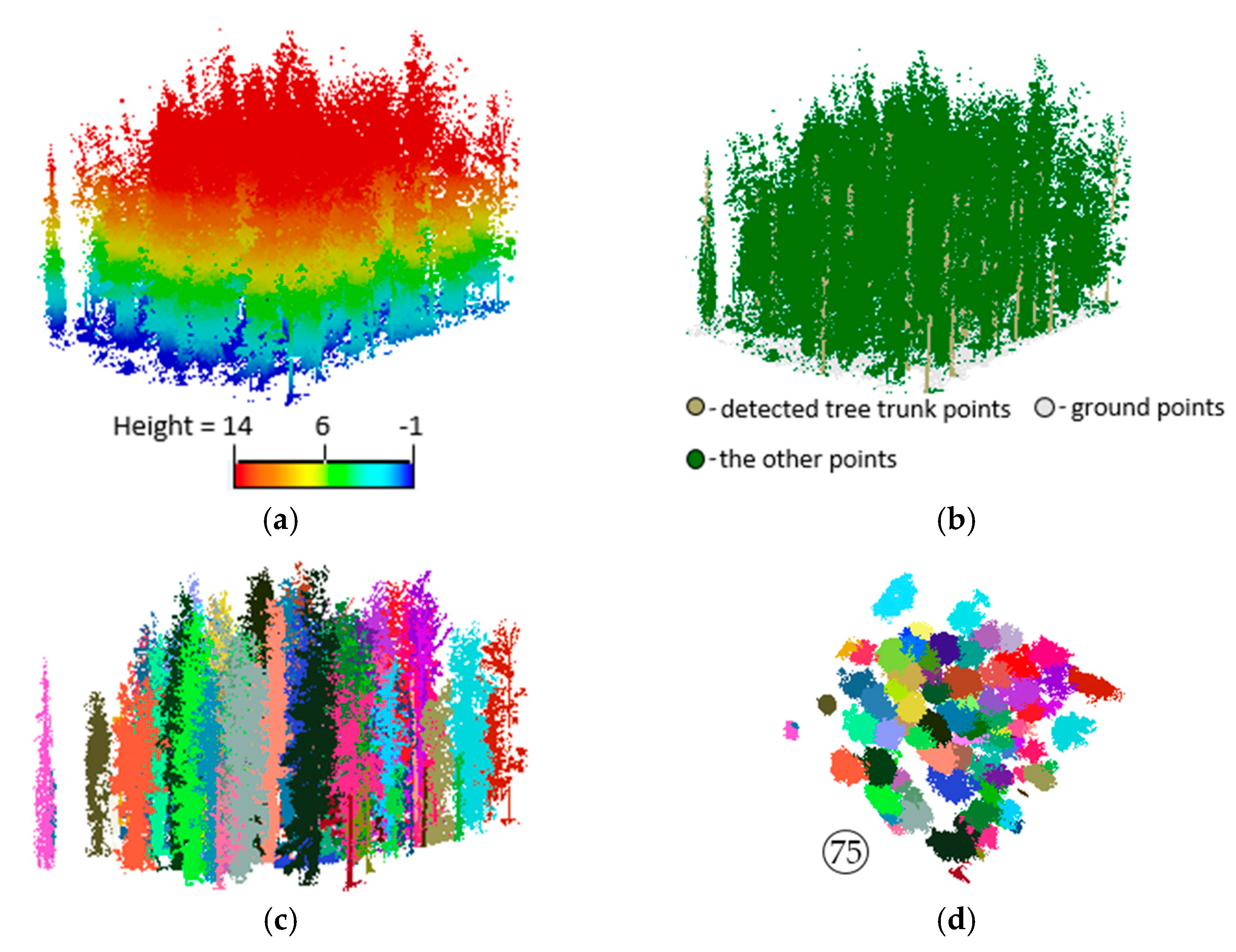
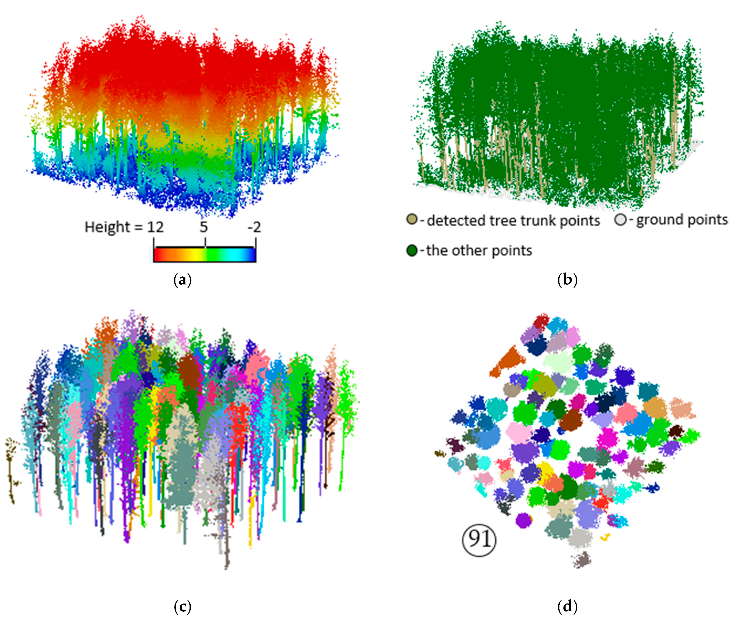
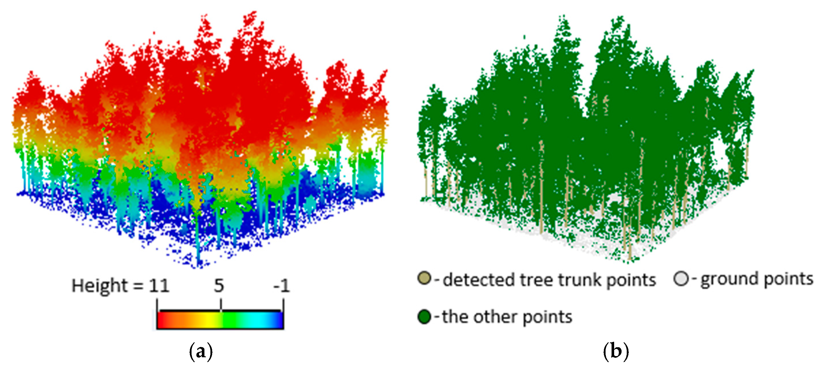
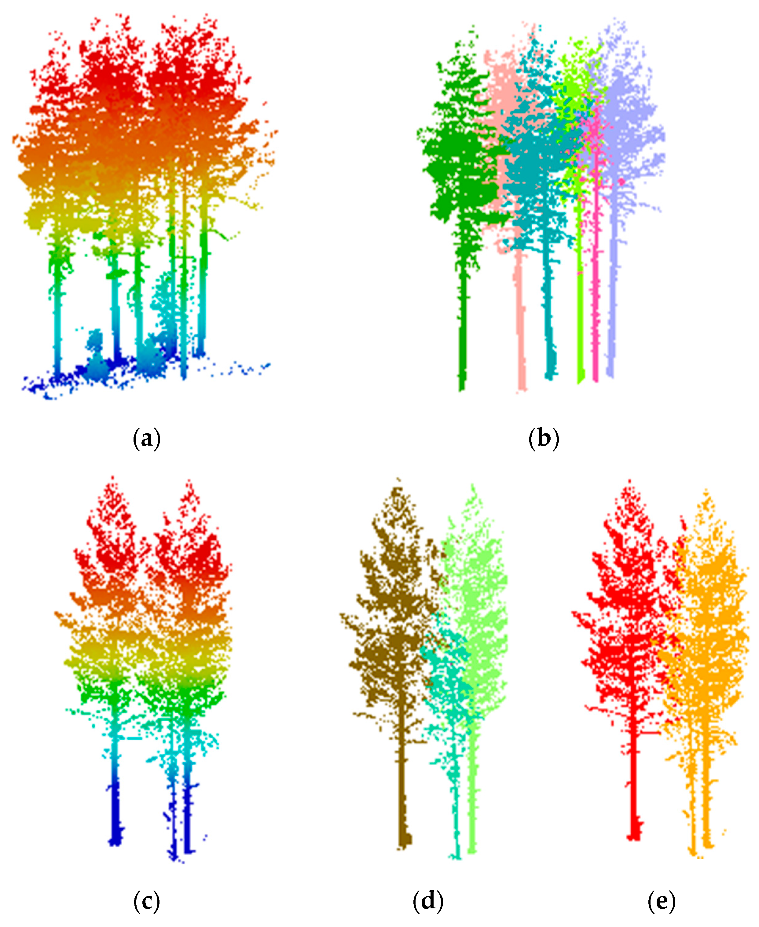
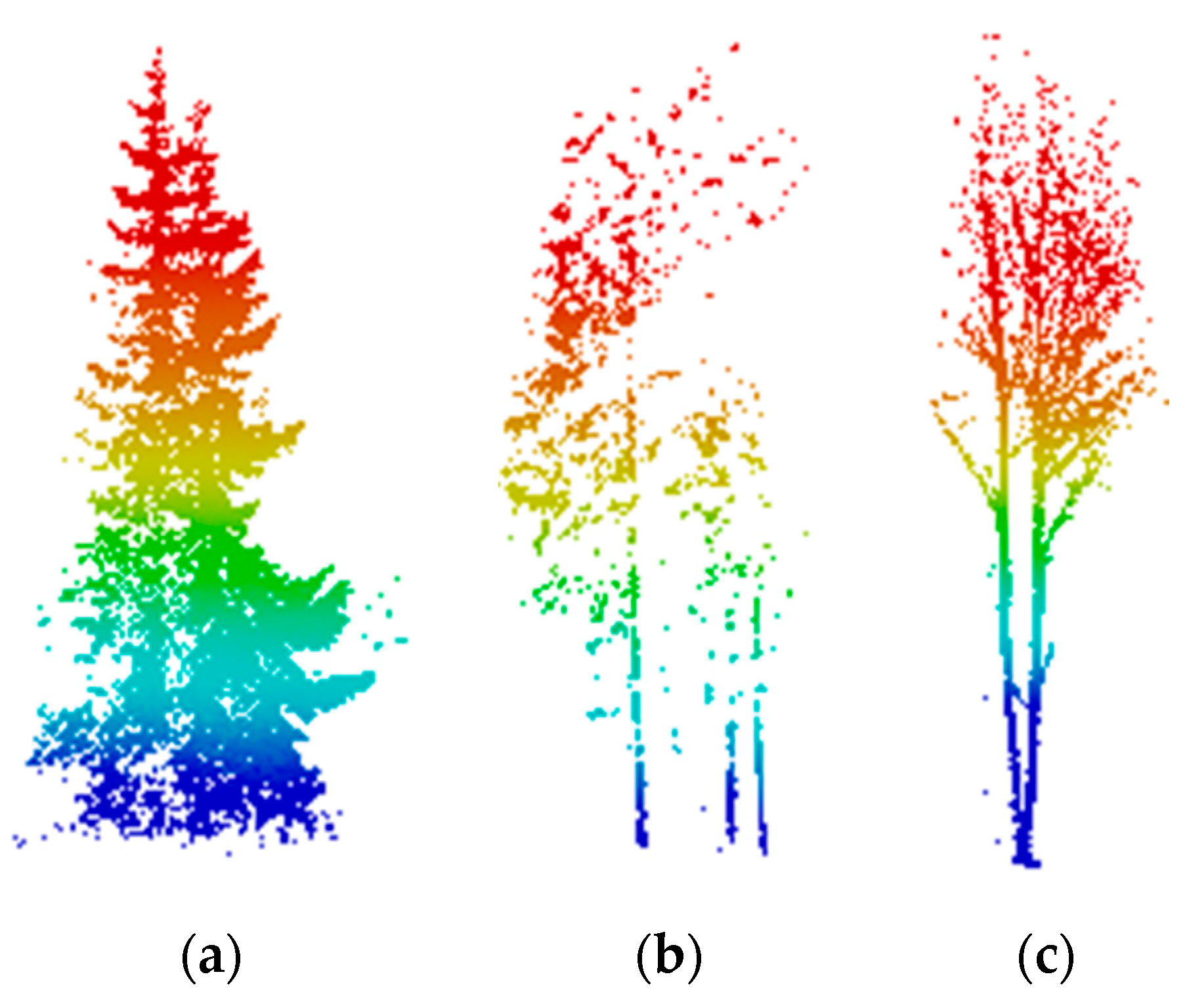
3.2. Extracting Results of Individual Trees

The values of six parameters required for the proposed method are listed in Table 2. The key procedures of trunk reorganization and crown point delineation for the five datasets are illustrated in Figure 6. The individual trees’ extraction results of five different TLS forest datasets are exhibited both in top and side view, respectively, where the top view results are attached with numbers denoting the number of detected trees.
Figure 6 illustrates the individual tree detection result at Plot 1. Tree detection results of Plots 2 to 5 are given in the Appendix. It can be seen that the tree trunks are well detected if the trunks are not seriously overlaid by branches, showing that the method works well in detecting trunks with recognizable shapes.
Figure 7 shows the connected tree detection results according to the hierarchical minimum cut operator. It can be seen that although the trees are distributed in a local dense forest area and tree crowns are connected and clumped, the individual trees are well detected. This is owed to two aspects. On the one hand, the well-detected tree trunks lay a key foundation for the hierarchical minimum cut operator for further extracting of the tree crowns. On the other hand, the hierarchical minimum cut operator successfully isolates the tree crown points corresponding to each tree trunk from the highest one to the lowest one. It can be seen that the minimum cut algorithm separates individual trees correctly in forest TLS point clouds. Figure 7 illustrates that the hierarchical minimum cut operator is effective and successful at isolating individual trees from a forest stand or plot area even with densely-connected or clumped trees. Particularly, as illustrated in Figure 7c,d, the closely-attached trees in a multi-layer canopy are also correctly segmented and detected. However, the little tree is not detected (as illustrated in Figure 7e) by the proposed methods of Lindenbergh et al. [39]. This demonstrates that the hierarchical minimum cut operator achieves an optimized segmentation result with the detected tree trunks as seed points, mitigating the possible under-segmentation in connected crowns and crowns in the in multi-layer canopy.
In light of the proposed methodological steps, the precondition of isolating tree crown points is highly required in order to correctly detect tree trunk points first. Hence, the trees may fail to be detected if the tree trunks do not show pole-like object shapes or the tree trunks are seriously occluded, as illustrated in Figure 8a,b. Accordingly, the crown points of the missed trunks may be segmented as the neighboring tree crowns if two tree trunks are closely distributed and one tree trunk fails to be detected. Another kind of error results from the segmentation of trees with a bifurcation at the bottom of the trunk. In this case, the tree will be spilt into two independent trees, as illustrated in Figure 8c.

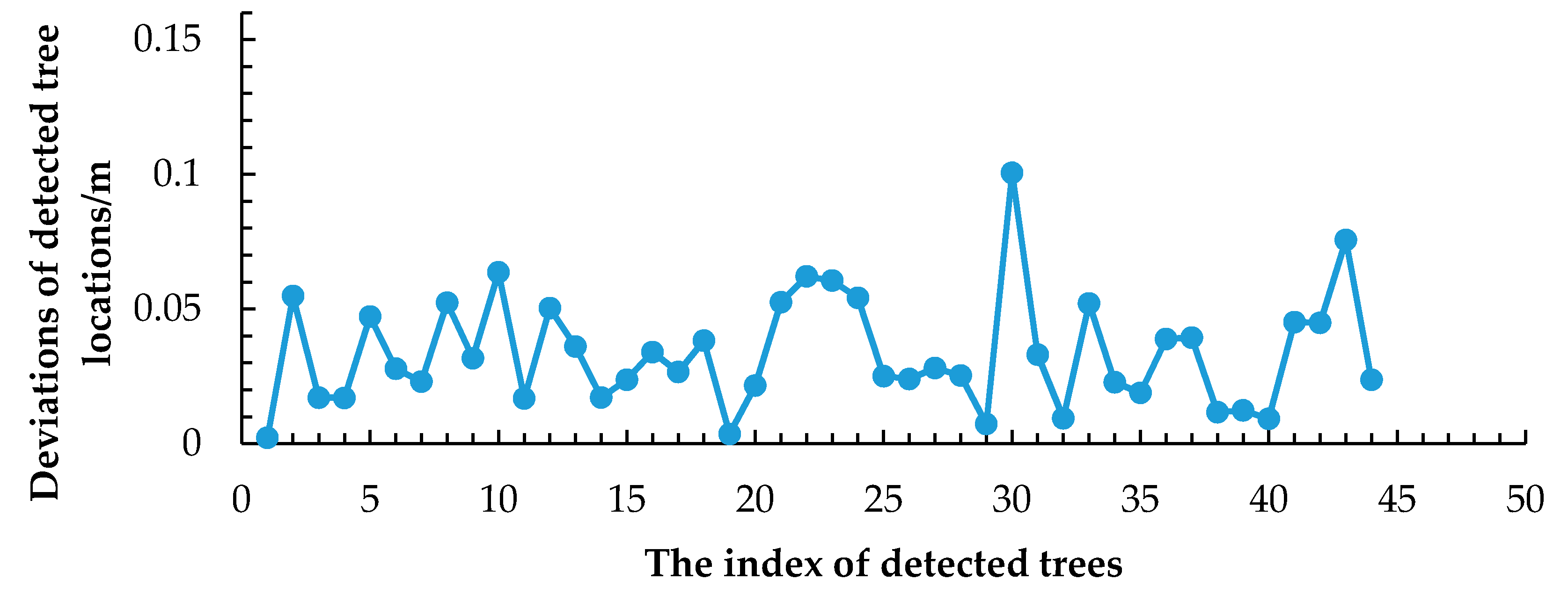
3.3. Accuracy Assessment and Evaluation of the Proposed Method

The parameters of the individual trees were calculated according to the detected results of the proposed method. We compared the calculated structure metrics at the individual tree levels of Plot 1 (tree location, height and DBH) with the ground truth and calculated the following factors to evaluate the proposed method.
  • TP (true positive): the number of trees detected with correct ground positions.
  • FP (false positive): when the trunk is not detected and missed and the corresponding tree crown is allocated to the neighboring trees.
  • FN (false negative): the number of ground truth trees undetected.
Moreover, the recall, precision and F-measure were also calculated for the evaluation of the proposed method.
r e c a l l    =    T P T P + F N × 100 %
p r e c i s i o n    =    T P T P + F P × 100 %
F - M e a s u r e    =    2 T P 2 T P + F P + F N × 100 %
Table 3 demonstrates the efficiency of the proposed method on the five processed datasets. It shows that the proposed method enables the detection of individual trees with higher TP numbers in most cases. On the other hand, the FPs are mainly contributed by the failed detection of tree trunks. For example, many tree trunks are missed because of non-pole-like shapes (as illustrated in Figure 8a) in Plot 5, resulting in a relatively low recall. The structure metrics (e.g., height, DBH) of trees were also calculated according to the individual tree detection results. Figure 9 and Figure 10 show comparisons between TLS-derived locations, tree heights and DBHs and field measurements in Plot 1.
The comparison in Figure 9 and Figure 10 shows that the locations of the trees in Plot 1 were correctly calculated by the proposed method. The comparison between the tree locations indicates that the maximum deviation is less than 0.11 m, showing the validity of the proposed method. Besides, the comparison between the tree heights indicates good consistency with field measurements. The comparison between DBHs also shows good consistency with field measurements. It also shows that three trees have big height differences with the field measurements. The visual inspection found that these trees are located near the border of Plot 1 and have sparse points on the tree crowns. The sparse points on the tree crowns are weakly connected according to the hierarchical minimum cut operator, resulting in the missing of tree crowns and the large deviation of height calculation. The regression analysis of tree heights shows that the R-squared values are 0.79 and 0.91 and the RMSEs are 1.25 m and 0.83 m with/without the three trees, respectively, as illustrated in Figure 11a,b. It shows that the proposed method estimates tree heights with good accuracy.

4. Conclusions

The paper proposes a novel method for isolating individual trees and calculates structure metrics at the individual tree level from large-scale forest scene point clouds. The trunks are recognized first by detecting the repetitive appearance of cylindrical segment units in the vertical direction. Then, they are used as markers to delineate individual trees by the proposed hierarchical minimum cut method. The hierarchical minimum cut method achieves good balance between over-segmentation and under-segmentation of tree point clouds, resulting in a successful detection of tree crown points from connected and clumped trees. The experimental studies show that the proposed method provides a powerful solution to isolate individual trees from TLS point in terms of accuracy and correctness. The individual tree detection from TLS point clouds also lay a good foundation for the accurate calculation of the structure metrics of trees, providing good datasets for biomass estimation and forest inventory.

Acknowledgments

This study was jointly supported by the National Natural Science Foundation of China (No. 41531177, No. 41371431) and the Specialized Research Fund for the Doctoral Program of Higher Education of China (No. 20120141110035).

Author Contributions

Bisheng Yang, Wenxia Dai, Zhen Dong developed the methodology and analyzed the data; Wenxia Dai, Zhen Dong conceived and performed the experiments; Yang Liu assisted with Section 2.1. All of the authors contributed to the writing and reviewing of the manuscript.

Conflicts of Interest

The authors declare no conflict of interest.

Appendix

The following Figure A1, Figure A2, Figure A3 and Figure A4 illustrate the individual tree detection results of Plots 2 to 5. For each plot, (a) displays the original point cloud colored by height level, (b) displays the trunk detection results, where the detected trunks are marked brown, the ground points are marked gray and the other points are marked green, (c) displays the side view of the individual tree detection results, where detected trees are randomly colored and the same color represents one tree, and (d) displays the top view of the individual tree detection results, where the number represents the number of detected trees.
Figure A1. Key procedures in individual tree detection of Plot 2. (a) The original TLS point clouds; (b) trunk detection result; (c) side view of individual trees’ detection result, where detected trees are randomly colored and the same color represents one tree; (d) top view of individual trees’ detection result, where the number represents the number of detected trees.
Remotesensing 08 00372 g012
Figure A2. Key procedures in individual tree detection of Plot 3. (a) The original TLS point clouds; (b) trunk detection result; (c) side view of individual trees’ detection result, where detected trees are randomly colored and the same color represents one tree; (d) top view of individual trees’ detection result, where the number represents the number of detected trees.
Remotesensing 08 00372 g013
Figure A3. Key procedures in individual tree detection of Plot 4. (a) The original TLS point clouds; (b) trunk detection result; (c) side view of individual trees’ detection result, where detected trees are randomly colored and the same color represents one tree; (d) top view of individual trees’ detection result, where the number represents the number of detected trees.
Remotesensing 08 00372 g014aRemotesensing 08 00372 g014b
Figure A4. Key procedures in individual tree detection of Plot 5. (a) The original TLS point clouds; (b) trunk detection result; (c) side view of individual trees’ detection result, where detected trees are randomly colored and the same color represents one tree; (d) top view of individual trees’ detection result, where the number represents the number of detected trees.
Remotesensing 08 00372 g015

References

  1. Hyyppä, J.; Kelle, O.; Lehikoinen, M.; Inkinen, M. A segmentation-based method to retrieve stem volume estimates from 3-D tree height models produced by laser scanners. IEEE Trans. Geosci. Remote Sens. 2001, 39, 969–975. [Google Scholar] [CrossRef]
  2. He, Q.; Chen, E.; An, R.; Li, Y. Above-ground biomass and biomass components estimation using LiDAR data in a coniferous forest. Forests 2013, 4, 984–1002. [Google Scholar] [CrossRef]
  3. Yang, X.; Strahler, A.H.; Schaaf, C.B.; Jupp, D.L.B.; Yao, T.; Zhao, F.; Wang, Z.; Culvenor, D.S.; Newnham, G.J.; Lovell, J.L.; et al. Three-dimensional forest reconstruction and structural parameter retrievals using a terrestrial full-waveform LiDAR instrument (Echidna®). Remote Sens. Environ. 2013, 135, 36–51. [Google Scholar] [CrossRef]
  4. Lin, Y.; Hyyppä, J.; Jaakkola, A.; Yu, X. Three-level frame and RD-schematic algorithm for automatic detection of individual trees from MLS point clouds. Int. J. Remote Sens. 2012, 33, 1701–1716. [Google Scholar] [CrossRef]
  5. Zhang, C.; Zhou, Y.; Qiu, F. Individual tree segmentation from LiDAR point clouds for urban forest inventory. Remote Sens. 2015, 7, 7892–7913. [Google Scholar] [CrossRef]
  6. Unger, D.R.; Hung, I.K.; Brooks, R.; Williams, H. Estimating number of trees, tree height and crown width using LiDAR data. GISci Remote Sens. 2014, 51, 227–238. [Google Scholar] [CrossRef]
  7. Srinivasan, S.; Popescu, S.C.; Eriksson, M.; Sheridan, R.D.; Ku, N.W. Terrestrial Laser Scanning as an effective tool to retrieve tree level height, crown width, and stem diameter. Remote Sens. 2015, 7, 1877–1896. [Google Scholar] [CrossRef]
  8. Henning, J.G.; Radtke, P.J. Detailed stem measurements of standing trees from ground-based scanning LiDAR. For. Sci. 2006, 52, 67–80. [Google Scholar]
  9. Liang, X.; Hyyppä, J.; Kankare, V.; Holopainen, M. Stem curve measurement using terrestrial laser scanning. In Proceedings of the 11th International Conference on LiDAR Applications for Assessing Forest Ecosystems, SilviLaser 2011, Hobart, Tasmania, Australia, 16–20 October 2011.
  10. Strîmbu, V.F.; Strîmbu, B.M. A graph-based segmentation algorithm for tree crown extraction using airborne LiDAR data. ISPRS J. Photogramm. Remote Sens. 2015, 104, 30–43. [Google Scholar] [CrossRef]
  11. Mongus, D.; Zalik, B. An efficient approach to 3D single tree-crown delineation in LiDAR data. ISPRS J. Photogramm. Remote Sens. 2015, 108, 219–233. [Google Scholar] [CrossRef]
  12. Lee, H.; Slatton, K.C.; Roth, B.E.; Cropper, W.P., Jr. Adaptive clustering of airborne LiDAR data to segment individual tree crowns in managed pine forests. Int. J. Remote Sens. 2010, 31, 117–139. [Google Scholar] [CrossRef]
  13. Popescu, S.C.; Zhao, K. A voxel-based LiDAR method for estimating crown base height for deciduous and pine trees. Remote Sens. Environ. 2008, 112, 767–781. [Google Scholar] [CrossRef]
  14. Holmgren, J.; Persson, A. Identifying species of individual trees using airborne laser scanner. Remote Sens. Environ. 2004, 90, 415–423. [Google Scholar] [CrossRef]
  15. Estornell, J.; Velázquez-Martí, B.; López-Cortés, I.; Salazar, D.; Fernández-Sarría, A. Estimation of wood volume and height of olive tree plantations using airborne discrete-return LiDAR data. GISci Remote Sens. 2014, 51, 17–29. [Google Scholar] [CrossRef]
  16. Hecht, R.; Meinel, G.; Buchroithner, M.F. Estimation of urban green volume based on single-pulse LiDAR data. IEEE Trans. Geosci. Remote Sens. 2008, 46, 3832–3840. [Google Scholar] [CrossRef]
  17. Lee, S.J.; Kim, J.R.; Choi, Y.S. The extraction of forest CO2 storage capacity using high-resolution airborne LiDAR data. GISci Remote Sens. 2013, 50, 154–171. [Google Scholar]
  18. Lin, Y.; Jaakkola, A.; Hyyppä, J.; Kaartinen, H. From TLS to VLS: Biomass estimation at individual tree level. Remote Sens. 2010, 2, 1864–1879. [Google Scholar] [CrossRef]
  19. Olsoy, P.J.; Glenn, N.F.; Clark, P.E.; Derryberry, D.R. Above ground total and green biomass of dryland shrub derived from terrestrial laser scanning. ISPRS J. Photogramm. Remote Sens. 2014, 88, 166–173. [Google Scholar] [CrossRef]
  20. Seidel, D.; Albert, K.; Ammer, C.; Fehrmann, L.; Kleinn, C. Using terrestrial laser scanning to support biomass estimation in densely stocked young tree plantations. Int. J. Remote Sens. 2013, 34, 8699–8709. [Google Scholar] [CrossRef]
  21. Rahman, M.Z.A.; Gorte, B.G.H.; Bucksch, A.K. A new method for individual tree delineation and undergrowth removal from high resolution airborne LiDAR. In Proceedings of the ISPRS Workshop on Laser Scanning 2009, Paris, France, 1–2 September 2009.
  22. Dassot, M.; Constant, T.; Fournier, M. The use of terrestrial LiDAR technology in forest science: Application fields, benefits and challenges. Ann. For. Sci. 2011, 68, 959–974. [Google Scholar] [CrossRef]
  23. Yu, X.; Hyyppä, J.; Vastaranta, M.; Holopainen, M.; Viitala, R. Predicting individual tree attributes from airborne laser point clouds based on the random forests technique. ISPRS J. Photogramm. Remote Sens. 2011, 66, 28–37. [Google Scholar] [CrossRef]
  24. Alonzo, M.; Bookhagen, B.; Roberts, D.A. Urban tree species mapping using hyperspectral and LiDAR data fusion. Remote Sens. Environ. 2014, 148, 70–83. [Google Scholar] [CrossRef]
  25. Chen, Q.; Baldocchi, D.; Gong, P.; Kelly, M. Isolating individual trees in a Savanna woodland using small footprint LiDAR data. Photogramm. Eng. Remote Sens. 2006, 72, 923–932. [Google Scholar] [CrossRef]
  26. Tao, S.; Wu, F.; Guo, Q.; Wang, Y.; Li, W.; Xue, B.; Hu, X.; Li, P.; Tian, D.; Li, C.; et al. Segmenting tree crowns from terrestrial and mobile LiDAR data by exploring ecological theories. ISPRS J. Photogramm. Remote Sens. 2015, 110, 66–76. [Google Scholar] [CrossRef]
  27. Liang, X.; Litkey, P.; Hyyppä, J.; Kaartinen, H.; Vastaranta, M.; Holopainen, M. Automatic stem mapping using single-scan terrestrial laser scanning. IEEE Trans. Geosci. Remote Sens. 2012, 50, 661–670. [Google Scholar] [CrossRef]
  28. Arachchige, N.H. Automatic tree stem detection-a geometric feature based approach for MLS point clouds. Int. Arch. Photogramm. Remote Sens. Spat. Inf. Sci. 2013, 1, 109–114. [Google Scholar] [CrossRef]
  29. Xia, S.; Wang, C.; Pan, F.; Xi, X.; Zeng, H.; Liu, H. Detecting stems in dense and homogeneous forest using single-scan TLS. Forests 2015, 6, 3923–3945. [Google Scholar] [CrossRef]
  30. Lalonde, J.F.; Vandapel, N.; Huber, D.F.; Hebert, M. Natural terrain classification using three-dimensional ladar data for ground robot mobility. J. Field Robot. 2006, 23, 839–862. [Google Scholar] [CrossRef]
  31. Rutzinger, M.; Pratihast, A.K.; Elberink, S.O.; Vosselman, G. Detection and modelling of 3D trees from mobile laser scanning data. Int. Arch. Photogramm. Remote Sens. Spat. Inf. Sci. 2010, 38, 520–525. [Google Scholar]
  32. Olofsson, K.; Holmgren, J.; Olsson, H. Tree stem and height measurements using Terrestrial Laser Scanning and the RANSAC algorithm. Remote Sens. 2014, 6, 4323–4344. [Google Scholar] [CrossRef]
  33. Sirmacek, B.; Lindenbergh, R. Automatic classification of trees from laser scanning point clouds. In Proceedings of the International Archives of the Photogrammetry, Remote Sensing and Spatial Information Sciences, ISPRS Geospatial Week 2015, La Grande Motte, France, 28 September–3 October 2015.
  34. Hernández, J.; Marcotegui, B. Point cloud segmentation towards urban ground modeling. In Proceedings of the 5th GRSS, ISPRS Joint Workshop on Remote Sensing and Data Fusion over Urban Areas, Shanghai, China, 20–22 May 2009.
  35. Boykov, Y.; Funka-Lea, G. Graph cuts and efficient ND image segmentation. Int. J. Comput. Vis. 2006, 70, 109–131. [Google Scholar] [CrossRef]
  36. Boykov, Y.Y.; Jolly, M.P. Interactive graph cuts for optimal boundary & region segmentation of objects in ND images. In Proceedings of the International Conference on Computer Vision, Vancouver, BC, Canada, 7–14 July 2001.
  37. Golovinskiy, A.; Funkhouser, T. Minimum cut based segmentation of point clouds. In Proceedings of the 2009 IEEE 12th International Conference Computer Vision Workshops (ICCV Workshops), Kyoto, Japan, 27 September–4 October 2009.
  38. Oesau, S.; Lafarge, F.; Alliez, P. Indoor scene reconstruction using feature sensitive primitive extraction and graph-cut. ISPRS J. Photogramm. Remote Sens. 2014, 90, 68–82. [Google Scholar] [CrossRef]
  39. Lindenbergh, R C.; Berthold, D.; Sirmacek, B.; Wang, J.; Ebersbach, D. Automated large scale parameter extraction of road-side trees sampled by a laser mobile mapping system. In Proceedings of the International Archives of the Photogrammetry, Remote Sensing and Spatial Information Sciences, ISPRS Geospatial Week 2015, La Grande Motte, France, 28 September–3 October 2015.
Figure 1. Workflow outline of individual tree extraction.
Remotesensing 08 00372 g001
Figure 2. Point cloud slicing and clustering results. (a) The horizontal slices (marked blue); (b) clustering results of each slice. The clustering results are randomly colored, and the same color represents a segment.
Remotesensing 08 00372 g002
Figure 3. Trunk extraction and tree location determination. (a) The cylinder segments marked in green color; (b) the detected trunk dotted in blue color; (c) the location of the tree dotted in red color.
Remotesensing 08 00372 g003
Figure 4. A binary segmentation example of nine points via G (V, E, W).
Remotesensing 08 00372 g004
Figure 5. Single tree segmentation by the hierarchical minimum cut method. (a) Side view of the cylindrical buffer zone (marked green) selected from the original point clouds to join the candidate tree segmentation, where points beyond the cylinder buffer zone are marked blue and candidate tree trunk points are marked brown; (b) the points within the buffer zone (the red cylinder area in (a)); (c) foreground and background seed point setting for segmentation, where the candidate tree trunk points serve as foreground seeds (marked brown) and the other trunk points serve as background seeds (marked orange); (d) the segmentation result of the candidate tree.
Remotesensing 08 00372 g005
Figure 6. Key procedures in individual tree detection of Plot 1. (a) The original TLS point clouds; (b) trunk detection result, where the detected trunks are marked brown, the ground points are marked gray and the other points are marked green; (c) side view of individual trees’ detection result, where detected trees are randomly colored and the same color represents one tree; (d) top view of individual trees’ detection result, where the number represents the number of detected trees.
Remotesensing 08 00372 g006
Figure 7. The detection results of trees with connected and clumped crowns by the hierarchical minimum cut algorithm. (a) The original point cloud of Test Data 1, where trees are distributed in a local dense area and tree crowns are connected and clumped; (b) the individual tree detection result of Test Data 1 by the hierarchical minimum cut; (c) the original point cloud of Test Data 2, where tree crowns are connected and in a multi-layer canopy; (d) the individual tree detection result of Test Data 2 by the hierarchical minimum cut; (e) the individual tree detection result of Test Data 2 by Lindenbergh et al. [39].
Remotesensing 08 00372 g007
Figure 8. Typical failure cases of our method. (a) The missing detection of a trunk because of non-pole-like shapes; (b) the fragmentized trunk structure failed detection because of the occlusions; (c) the trunk is bifurcated at the bottom and spilt into two trees.
Remotesensing 08 00372 g008
Figure 9. Deviations of detected tree locations and field observation.
Remotesensing 08 00372 g009
Figure 10. Comparison of tree metrics acquired from TLS analysis and field observation. (a) Tree height comparison; (b) DBH comparison.
Remotesensing 08 00372 g010
Figure 11. Scatterplot of regression result for field measurement and TLS-derived tree heights of the 44 detected trees (a) and 41 detected trees that are not located at the boundary of the plot (b).
Remotesensing 08 00372 g011
Table 1. Details of the TLS scanning data.
PlotPlot 1Plot 2Plot 3Plot 4Plot 5
Acquisition timeSummer, 2014
InstrumentLeica HDS6100
Field of view360° × 310°
Beam divergence0.22 mrad
Increment0.036° (horizontal)/0.036° (vertical)
Plot size32 m × 32 m
Number of points (million)47.1868.1132.8750.4269.12
Point density (points/cm2)4.97.33.55.27.7
Number of trees5280956759
Table 2. Parameters’ setting for experimental datasets.
ParameterDescriptorValue
HsliceThickness of horizontal slice0.2 m
rc_minMin radius of cylinder in trunk point extraction0.05 m
rc_maxMax radius of cylinder in trunk point extraction0.5 m
σThe average point span in Bp,q calculation1.0
kConstant value to determine the buffer zone as the input point cloud of the hierarchical minimum cut1.25
Weight(p,S)Weight of edges’ t-links connecting input points to terminal S0.8
Table 3. Detection rates of individual trees in five forest datasets.
PlotTPReference TreesFPFNRecallPrecisionF-Measure
147525590.38%90.38%90.38%
275807593.75%91.46%92.59%
391959495.79%91.00%93.33%
462676592.54%91.18%91.85%
5475971279.66%87.04%83.19%

