Article

Heterogeneous Fault Mechanisms of the 6 October 2008 MW 6.3 Dangxiong (Tibet) Earthquake Using Interferometric Synthetic Aperture Radar Observations

1
School of Geodesy and Geomatics, Wuhan University, Wuhan 430079, China
2
Key Laboratory of Geospace Environment and Geodesy, Ministry of Education, Wuhan 430079, China
3
Collaborative Innovation Center of Geospatial Technology, Wuhan 430079, China
*
Author to whom correspondence should be addressed.
Remote Sens. 2016, 8(3), 228; https://doi.org/10.3390/rs8030228
Submission received: 23 October 2015 / Revised: 25 February 2016 / Accepted: 1 March 2016 / Published: 12 March 2016
(This article belongs to the Special Issue Remote Sensing in Tibet and Siberia)

Abstract

:
Most current crustal deformation models do not account for topographic effects, crustal lateral variations, and complex fault geometries. To overcome these limitations, we apply finite element models constrained by interferometric Synthetic Aperture Radar (InSAR) images of co-seismic displacements to the 2008 Mw 6.3 Dangxiong earthquake that occurred in Yadong–Gulu rift, southern Tibet. For mountainous plateau environments, InSAR observations are advantageous for studying crustal deformation and crustal medium structure. We evaluate the effect of topography and variations in Poisson’s ratio and elastic moduli on estimation of coseismic deformation from InSAR observations. The results show that coseismic surface displacements are more sensitive to variations in Young’s modulus than to variations in topography and Poisson’s ratio. Therefore, with constant Poisson’s ratio and density, we change the Young’s modulus on each side of the fault to obtain the model that best fits the observations. This is attained when the Young’s moduli in the eastern and western sides of the fault were 2.6 × 10¹⁰ Pa and 7.8 × 10¹⁰ Pa, respectively. The result is consistent with previous field surveys that the medium on either side of the fault is different.

Graphical Abstract

1. Introduction

The development of space-based geodetic techniques including Global Positioning System (GPS) and Interferometric Synthetic Aperture Radar (InSAR) has allowed the observation of the deformation that occurs during earthquakes with an accuracy of mm and spatial resolution of m [1,2]. Based on the assumptions of an elastic half-space or a horizontally layered elastic half-space, the observations can be rapidly modeled by an analytical model or analytical and semi-analytical codes. Steketee [3] first introduced dislocation theory to the field of seismology. Following this, the analytical model of Okada [4] has been often employed in the form of a dislocation embedded in a homogeneous, isotropic, Poisson-solid half-space. More advanced models which account for crustal heterogeneity in horizontally layered elastic half-space were subsequently developed [5,6]. Although these analytical or semi-analytical models can rapidly reproduce the surface deformation and stress–strain distribution generated by faulting, they generally do not allow for topographic effects, lateral variations in the mechanical properties of the crust, or complex fault geometries. They may even be non-convergent and unsuitable in the near-field due to the assumption of extended sources modeled by a discrete distribution of point sources [7,8,9,10].
However, geological and geophysical data as well as seismic surveys indicate that the crust is elastically inhomogeneous with significant topographic relief [11,12]. According to the analysis of earthquakes, variations of the elastic modulus of the rock have a significant effect on the earthquake focal mechanism solutions including the slip pattern, source rupture complexity, and focal depth [13,14,15,16,17,18]. Moreover, the study of Williams and Wadge [9] showed that large topographic relief strongly affects the surface deformation predicted by elastic models. Using finite element models (FEMs), we can overcome these limitations of elastic homogeneity, the absence of topography, and planar fault geometries. Therefore, numerical models of faulting events were developed to invert a fault source with a non-uniform fault-slip distribution, taking into account the effect of topography and medium heterogeneity [19,20,21,22,23,24,25].
In this study, we use Synthetic Aperture Radar (SAR) images from Envisat ASAR and ALOS PALSAR to investigate the coseismic deformation and slip distribution of the Dangxiong earthquake. After interferometry processing, we constructed FEMs of the Mw 6.3 Dangxiong earthquake and evaluated the effects of topography and three-dimensional (3-D) variations in the elastic moduli on coseismic deformation estimation. Two topographic models, a flat surface and a realistic topographic surface, were used to evaluate the effects on slip distribution estimation. A comparison between the homogeneous model and heterogeneous model revealed the effect of the material’s inhomogeneities on the slip distribution. Next, we developed a procedure in which the heterogeneous slip distribution and the Young’s modulus between the eastern and western sides of the fault were estimated from the FEMs and InSAR data. Finally, we compared between FEMs of different configurations and explored the background of the seismogenic structure of the Dangxiong earthquake.

2. Methods

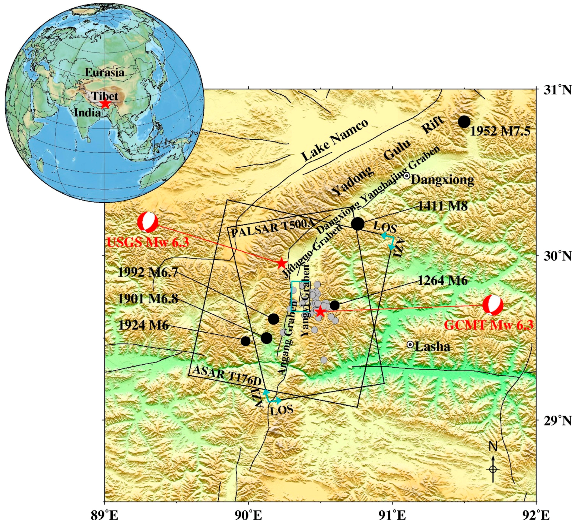
2.1. Study Area and Geological Background

The 6 October 2008 MW 6.3 Dangxiong earthquake occurred in Dangxiong County, Tibet Province, China, located in the central section of the Yadong–Gulu rift of southern Tibet (Figure 1). The earthquake can be attributed to crustal extensional deformation. The location of the main shock and the spatial distribution of aftershocks indicate that the north–south trending and crescent-shaped Yangyi graben is the seismogenic structure of the 2008 event [26]. The Yangyi graben is an active asymmetric half-graben, which forms the northern section of the Yadong–Gulu rift [27,28].
The Yadong–Gulu rift, which includes the Dangxiong Yangbajing Graben, Jidaguo Graben, Yangyi Graben, and Angang Graben, is a region of intensive tectonic activity. According to the Chinese earthquake catalogues [29,30], 14 earthquakes of M ≥ 6.0 occurred in the Yadong–Gulu rift zone on the Tibetan Plateau since 1264 A.D. [31]. Over the past decades, many researchers have analyzed the spatial distribution of these events and the crustal motion along the Yadong–Gulu rift, and the results show that since the 1952 event, strong earthquakes have been migrating southward along the Yadong–Gulu rift into the Yangyi and the Angang Grabens.
Extending from south to north across the Himalayas, the Yarlung–Zangbo suture, the Lhasa block, and the Nyainqentanglha lie sequentially. The Yadong–Gulu rift is one of the most active rifts in southern Tibet, where transverse extension can reach ~15–25 nstrain/y [32]. By using geological measurements, the average opening rate of the Yadong–Gulu rift was estimated by Armij et al., as 1.4 ± 0.8 mm/y [33], but the opening rate of the northernmost part of the rift may be as high as 15 mm/y [33]. However, based on more recent data from GPS surveys between 1991 and 2001, Chen et al., showed that the average opening rate of the Yadong–Gulu rift is much higher—about 6.5 ± 1.5 mm/y [27,28].
Furthermore, the wide distribution of the north–south rifts and normal and strike-slip faulting events across southern Tibet demonstrate that an east–west extension of inner Tibet occurred prior to the Dangxiong earthquake [34]. The continuing collision between the Indian continental plate and the Eurasian Plate has led to the east–west crustal extension, with the Dangxiong earthquake being one more manifestation of the ongoing collision process.
The 6 October 2008 Mw 6.3 Dangxiong earthquake caused considerable economic loss (about USD 41 million) and serious casualties (up to 10 people) [34]; hence, it has been the subject of many studies. Several studies used different observations and constraints, yet none of them accounted for the effect of topography and medium heterogeneities. However, a field investigation revealed that the topographic and geological structures differed between the eastern and western sides of the rupturing fault in the Dangxiong earthquake. The field survey showed that the western margin of the Yangyi graben consists of Miocene volcanic rocks, and the eastern margin is granite [24]. To overcome the simplified assumptions of uniform slip in a homogenous half-space in the fault models, we included the topography and medium heterogeneities in our FEM. The studies indicate that a better understanding of the mechanism of the Dangxiong earthquake will help us interpret the regional tectonic evolution and improve our estimates of potential devastating earthquakes occurring around the Yadong–Gulu rift [26,31].

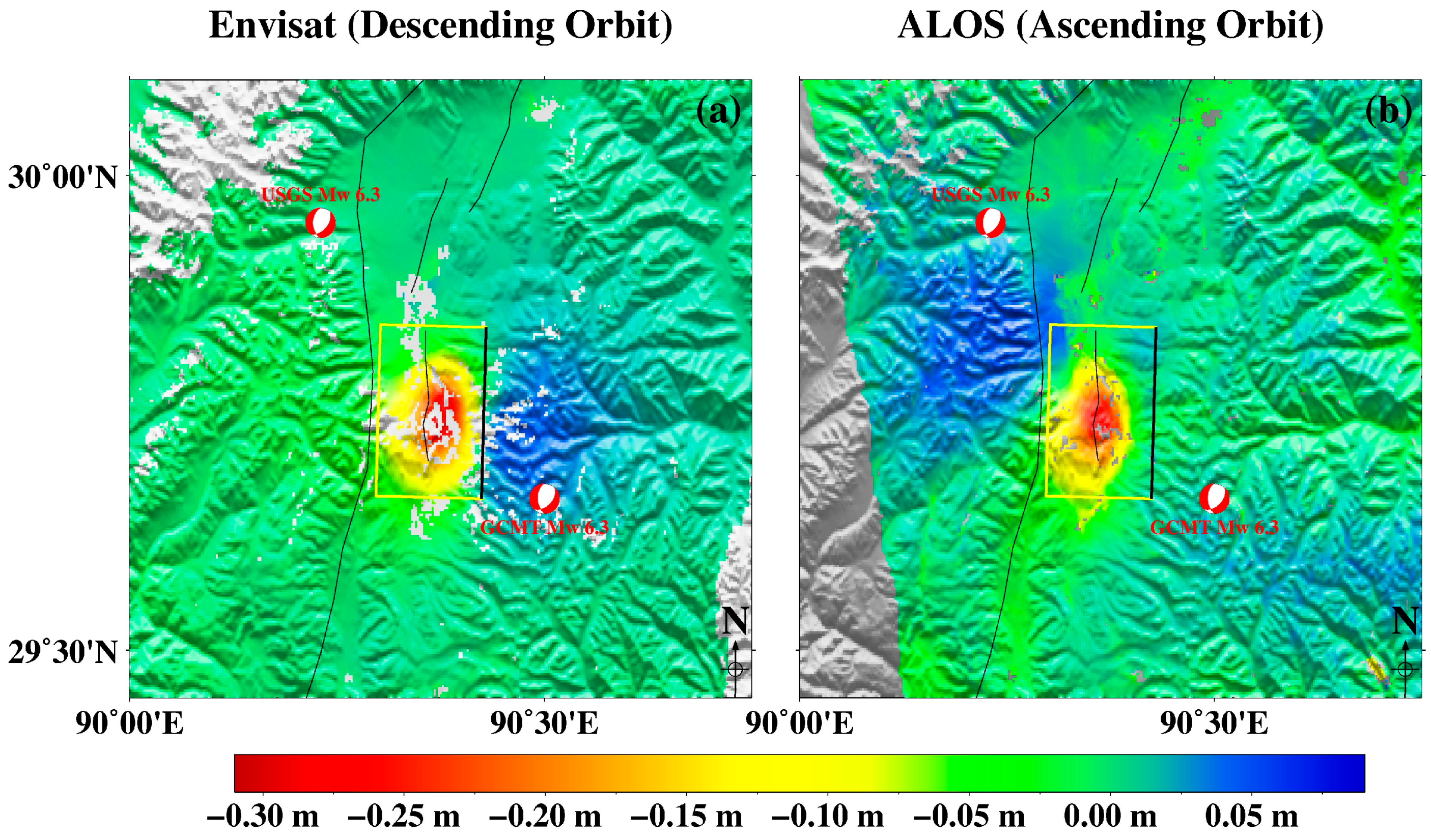
2.2. InSAR Observation and Coseismic Deformation

The coseismic deformation field obtained from the SAR images covering the main earthquake deformation zone was adopted in our study, which have already been published by Liu et al. [31]. As more than one radar look direction is needed to provide a reliable estimate of the slip along a rupture plane [14,37,38], a pair of ALOS Phased Array type L-band Synthetic Aperture Radar (PALSAR) images (Ascending Track 500) and a pair of ENVISAT Advanced Synthetic Aperture Radar (ASAR) images (Descending Track 176) were used to acquire the coseismic deformation field using the Caltech/JPL software ROI_PAC (version 3.1 beta) [39] in the two-pass differential interferometry mode (Table 1) [31]. The topographic phase was removed from the interferograms using the 3 arc-second (~90 m) Shuttle Radar Topography Mission (SRTM) digital elevation model (DEM). Precise orbits from ESA and JAXA were used to correct the interferograms for differences in satellite position. The interferograms were filtered using the power spectrum filter [40] to reduce the effects of phase noise and unwrapped using the branch cut method [41]. The interferograms were then geocoded to geographic coordinates. Finally, we obtained the coseismic deformation field from the geocoded interferograms (Figure 2) [31].
The coseismic deformation caused by the Dangxiong earthquake is evident in both the descending and ascending interferograms (Figure 2). The simple pattern of the deformation field suggests that there is only one fault geometry involved in the earthquake rupture. The coseismic deformation on the western side of the earthquake fault is considerably greater than on the eastern side, which suggests that the Dangxiong MW 6.3 event is mainly a dip-fault earthquake.

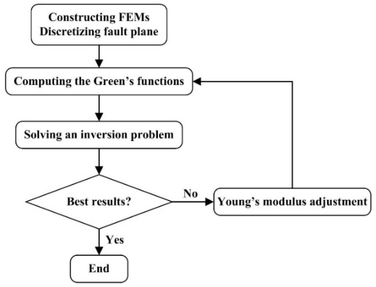
2.3. FEM-Based Inversion

To account for the topographic effects as well as the mechanical heterogeneities in the coseismic deformation inversion, the coseismic surface displacements and Green’s functions for the 3-D elastic models were computed by the finite element method. We constructed several FEMs using the Los Alamos Grid Toolbox (LaGriT) [43], a free library of user callable tools that provide mesh generation, mesh optimization and dynamic mesh maintenance, and computed the Green’s functions using PyLith [44], a parallel finite element code which can simulate lithospheric deformation over a wide range of spatial and temporal scales. The computational domain was designed with dimensions 200 × 200 × 310 km3 (Figure 3) to avoid artifacts in the numerical solution caused by the proximity of the external boundaries. The FEMs were constructed based on the fault geometry determined by Liu et al. [31] (Table 2). For the boundary conditions, the displacements on the outermost lateral boundaries and on the bottom are fixed to zero, while the boundary at the ground surface is stress-free [22]. The ground surface of the 3-D model with topographic relief was generated from a digital elevation model from the 3 arc-second (~90 m) Shuttle Radar Topography Mission (SRTM) data [45]. We downsampled the elevation to a grid spacing of less than 300 m in the near field of the 2008 coseismic rupture and gradually increased the grid size to 4 km in the far field (Figure 3 and Figure 4). Using LaGriT, the computational domain was meshed into 365,789 isoparametric and arbitrarily distorted tetrahedral elements connected by 66,789 nodes. The mesh resolution is about 500 m in the near field and decreases to 5 km in the far field (Figure 3). The rupture interface is partitioned into 441 split nodes which can introduce fault displacements into finite element numerical computations (20 × 20 fault patches of ~20 × 20 km size) to allow for a distribution of coseismic slip [46]. We divided our model into seven regions with potentially different density and Young’s modulus (Figure 3), with values based on data from the Crust 1.0 high-resolution model at 1 × 1 degrees [47]. The Crust 1.0 model is a seven layers one-dimensional model, but the thickness of some layers may be zero. The simulated 3-D domain includes a 76-km-thick continental crust which can be separated into three layers—the upper, middle, and lower crust of thickness 38, 18, and 20 km, respectively, and divided along the rupture into the eastern and western sides because of the different mediums on each side (Figure 3 and Table 3).
The common practice of estimating slip distribution on faults using geodetic data subdivides the fault surface into a finite number of patches and relates the geodetic observations at the top free surface to the slip on the patches through the equation
d = G ( m ) s + ε
where G is the matrix of the synthetic Green’s functions related to the LOS surface displacements d, m is the vector of the fault geometry parameters, s is the slip vector on the fault surface, and ε represents the normally distributed errors of mean 0 and covariance matrix d , ε~N(0, d ). The matrix G, generated by the FEMs, represents the relationship between the surface displacements and slip on the fault surface.
However, the inverse problem is generally ill posed and unstable because the fault is discretized into a large number of fault patches to achieve detailed slip distribution. In this case, the simple linear least-squares methods cannot give conforming slip values on adjacent patches. Thus, to obtain well posed and stable solutions of the inverse problem, it is necessary to introduce smoothing constraints which minimize the differences between neighboring dislocations. To obtain this, Xu et al. [48] re-formulated the objective function of the inverse problem
Φ ( s ) = d 1 / 2 ( d Gs ) 2 + λ 2 L s 2
where λ 2 is a regularization parameter, namely a trade-off between minimizing the data misfit d 1 / 2 ( d G s ) 2 and the regularizing functional L s ) 2 . The matrix L is a Laplacian operator, and the finite difference approximation of the Laplacian operator is
2 s = 0 s i 1 , j 2 s i , j + s i + 1 , j ( Δ x ) 2 + s i , j 1 2 s i , j + s i , j + 1 ( Δ y ) 2
where Δ x and Δ y are the along-strike and surface projection of the downdip fault patch dimensions, respectively.
Thus, the inverse problem is equivalent to an optimization problem in which one seeks the slip distribution, s, that minimizes the objective function, given a specific value of λ2 [49,50,51]. To constrain large variations between adjacent patches, the value of λ2 must be chosen to balance the relative importance of fitting the observations and the regularizing function. The L-curve criterion [52] is used to determine the value of λ2 in this work. Negative constraints are introduced to the dip-slip, while no constraints are used to strike-slip in this inversion. According to previous studies, the event is a normal faulting accompanied by a strike-slip component, so the tensile component is not taken into consideration.
To invert the heterogeneous fault mechanism of the Dangxiong earthquake, we developed a procedure that estimates the heterogeneous slip distribution and the Young’s modulus between the eastern and western sides of the fault based on the FEMs and the ground deformation data. The procedure can be split into four main modules: (i) constructing the FEMs and discretizing the fault plane into a finite number of patches; (ii) assuming unit slip over each patch and computing the Green’s functions for static displacements using FEMs; (iii) solving an inversion problem to determine the slip distribution using a quadratic programming algorithm with bound constraints on the slip values and (iv) changing the Young’s modulus between the eastern and western side of the fault and repeating (ii) and (iii) with the same smoothing factor to obtain the best-fit results (Figure 5).

3. Examining the Sensitivity of Coseismic Deformation to Changes in the Topographic Relief, Poisson’s Ratio, and Young’s Modulus

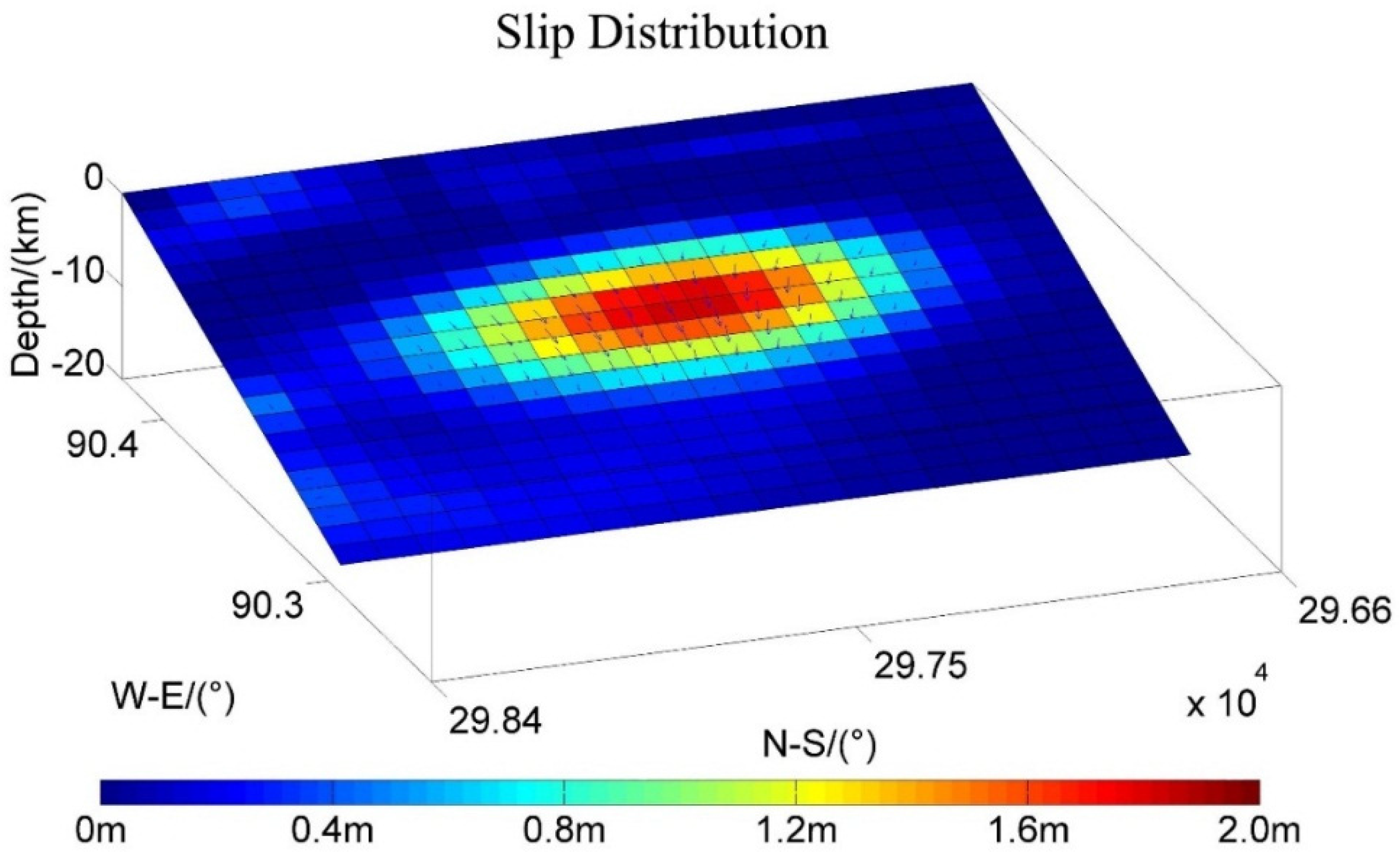
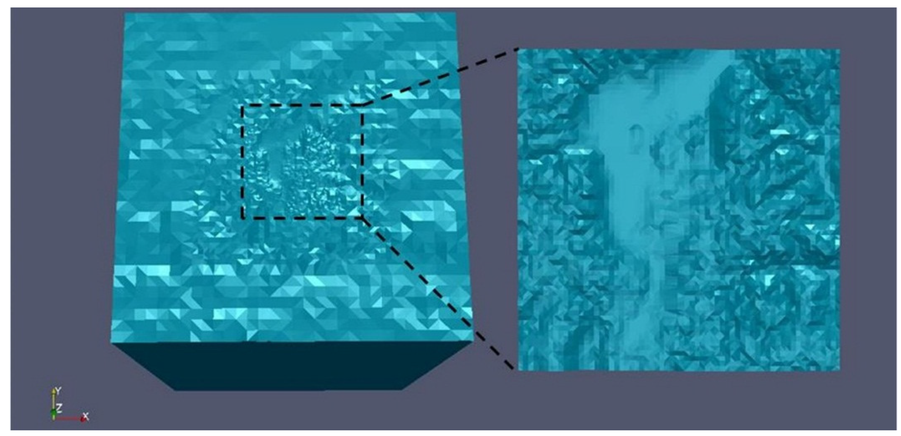
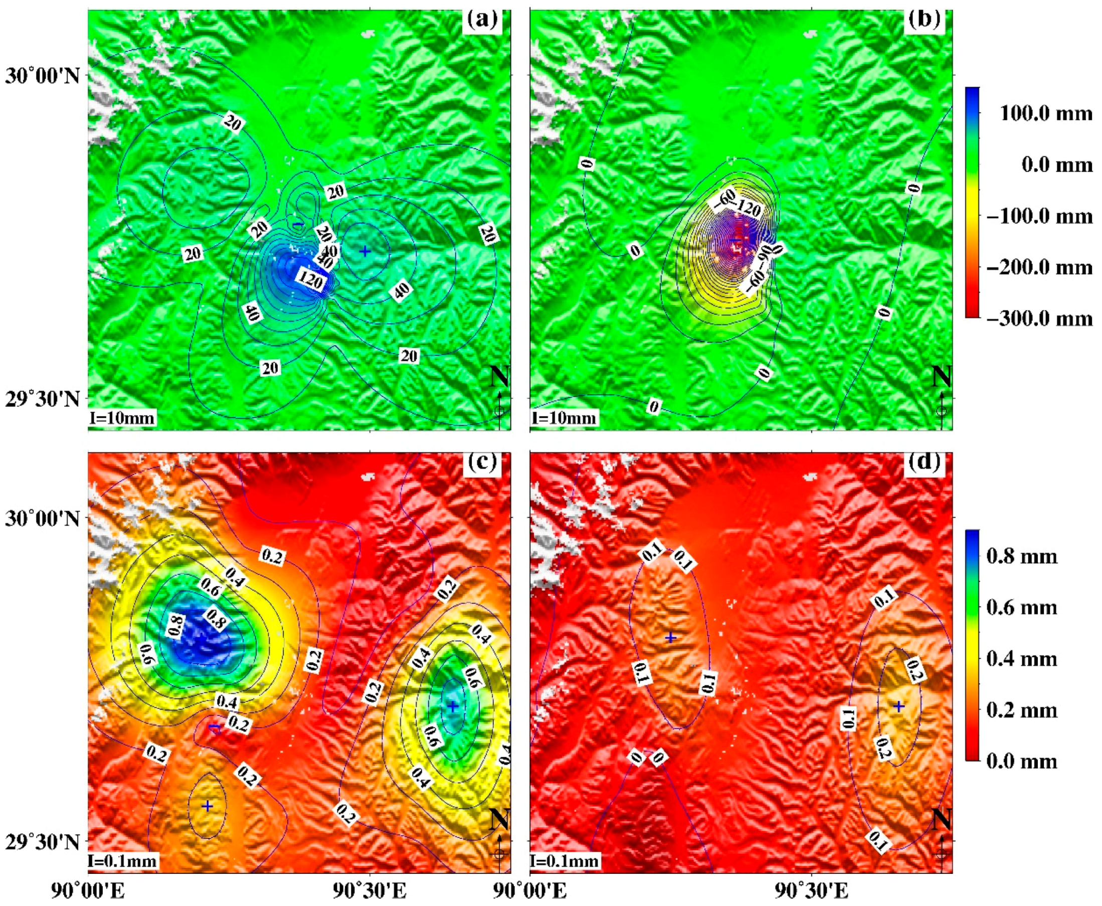
3.1. Effect of Topography on Slip Distribution

Although topography has a large effect on the results predicted by elastic deformation models in regions of significant relief [9,53,54], slip distributions’ inversions with an elastic half-space or a horizontally layered elastic half-space models often do not account for the effect of topographic relief. The maximum topographic relief around the 2008 earthquake zone was 3.5 km (Figure 1). To examine the effect of topographic relief on the coseismic deformation of the 2008 event, we constructed two FEMs, one with a flat free surface and the other with a free surface which was interpolated from the SRTM model; all the other parameters of the two models were equal. To forward simulation of coseismic deformation of the 2008 earthquake, a slip distribution was estimated by FEMs with flat topography. By using this slip distribution to the two FEMs, we can compare the coseismic surface displacements from a model with a flat surface to that with a realistic topographic relief.
As shown in Figure 6, the differences in coseismic surface displacements, whether horizontal or vertical, between the two models appeared mainly at the mountainous zone where the topographic relief is large, thus confirming that the topographic relief cannot be neglected. The horizontal and vertical displacements predicted by the model with a realistic topography are generally smaller than those from the flat earth model (Figure 6b,c); thus, the difference between them is positive because of the negative displacements caused by the normal dip-slip with only a small component of right-lateral strike-slip. The results indicate that the predicted displacements in the flat earth model are overestimated. Although the maximum difference between these two models is only about 3%, these differences are systematic errors. Therefore, when implementing inversion schemes, models with realistic topographic relief will provide more realistic results.

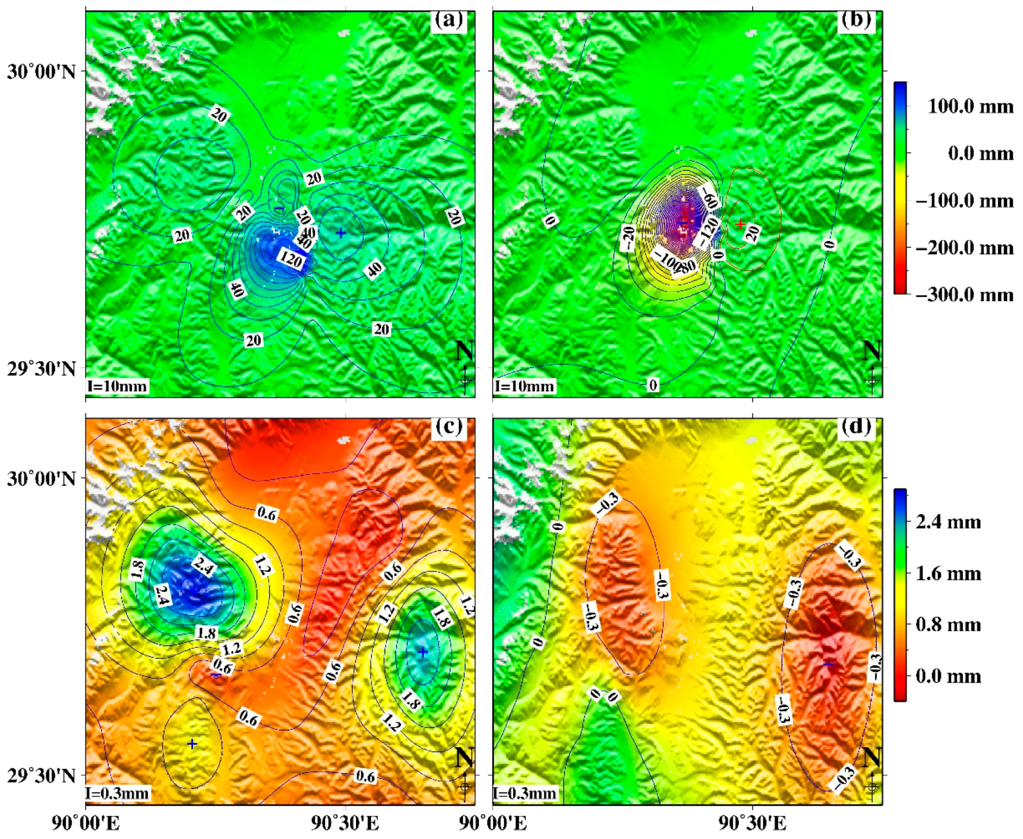
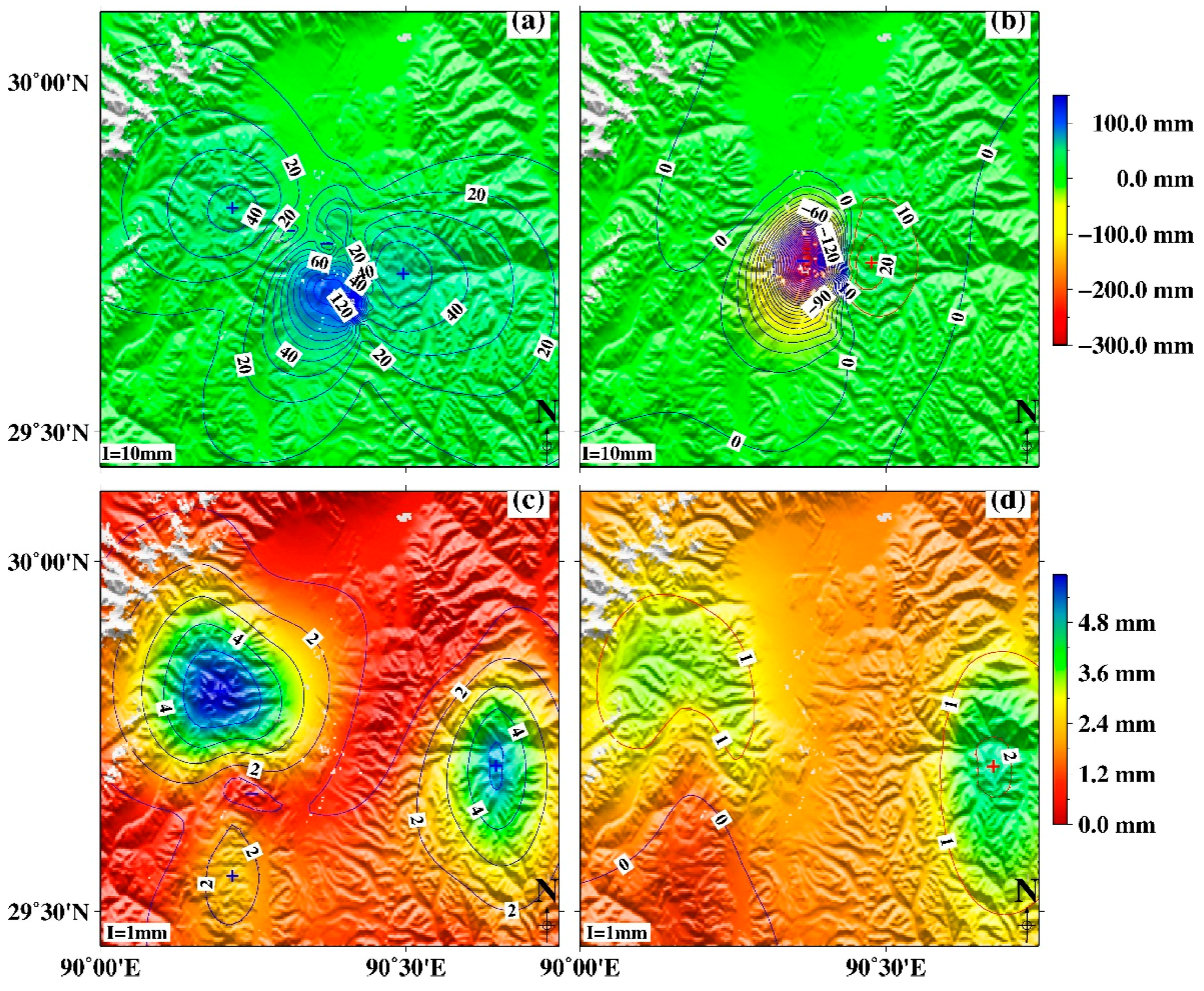
3.2. Impact of Heterogeneous Elastic Models on Slip Distribution

The Poisson-solid assumption in dislocation models (i.e., Poisson’s ratio of 0.25) is not representative of crustal rocks because Poisson’s ratio increases with fluid content and pressure and varies according to the fluid content and rock composition [55]. To examine the effect of Poisson’s ratio on the coseismic deformation caused by the 2008 earthquake, we calculate the surface coseismic displacements with a Poisson’s ratio of 0.25 and 0.3, respectively, using the same input slip distribution model. The maximum difference in displacement between these two models is about 5%, and the differences in horizontal and vertical displacements display opposite tendencies (Figure 7).
Geologic observations, shear wave splitting, and laboratory measurements indicate that the elastic properties of the lithosphere are generally heterogeneous [56,57,58,59,60]. A field survey showed that the geological structure east of the fault rupture caused by the 2008 earthquake is different from that on the west sides of the fault rupture [26]. To examine the influence of elastic heterogeneity on the coseismic deformation, we calculate the surface coseismic displacements with Young’s modulus values of 9 × 10¹⁰ Pa and 4 × 10¹⁰ Pa, using the same input slip distribution model. The surface displacements (Figure 8) are more sensitive to variations in Young’s modulus than to variations in the topography and Poisson’s ratio (Figure 6 and Figure 7). The maximum difference between the two models is 35%. Owing to this sensitivity to Young’s modulus, we attribute the medium heterogeneity mainly to variations in the Young’s modulus.

4. Results and Discussion

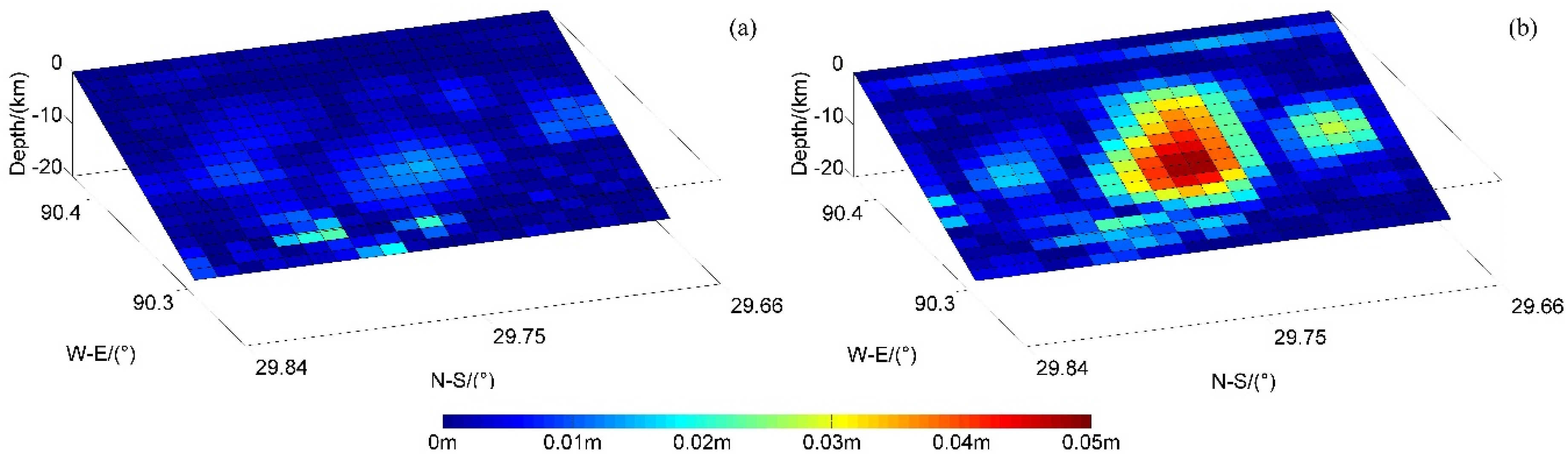
4.1. Inverted Coseismic Slip and Young’s Modulus from a Heterogeneous Elastic Model

Based on the FEM inversion method, Masterlark et al. [61] pointed out that models that assume homogeneous elastic half spaces significantly overestimate the coseismic displacements; therefore, models with heterogeneous material properties are necessary. Similarly, FEM simulation of subduction thrusting and comparisons conducted by Zhao et al. [8] indicate that rigid crustal layering and lateral variations have a significant effect on surface deformation. In a study of the Sumatra subduction zone, Hsu et al. [23] noted that the discrepancies between homogeneous and heterogeneous models are strongly dependent on the contrast of the elastic properties between the two sides of the fault; from the root mean square (rms) we can deduce whether the models match the true crustal structure.
However, the Green’s functions generated from the FEM with topography (Figure 4) and the material properties configuration from Crust 1.0 (Table 3) account only for the effect of the rigid crustal layering and topographic relief, while the effect of lateral variations was neglected. The material’s properties can be determined by physical parameters such as density, Poisson’s ratio, and Young’s modulus. However, studies have shown that the crustal properties are dominated by Young’s modulus, with density and Poisson’s ratio having little effect on the deformation characteristics [53,62,63]. Therefore, in this study we constructed the HEterogeneous with Topography (HET) model which has a different Young’s modulus on each side of the rupture fault.
To account for the layered nature of the crust, we separate the crust into three layers: the upper, middle, and lower crust layers, of thickness 38, 18, and 20 km, respectively, based on the Crust 1.0 model [47]. The fault length and width are extended to 20 km along the strike and down-dip directions; thus, the fault is entirely contained in the upper layer. We examined the effect of the Poisson’s ratio and Young’s modulus in the middle and bottom layers of the crust on coseismic deformation. The results show that they have little effect on coseismic deformation; thus, we do not need to account for the effect of lateral variations in the two lower layers of our model.
The data used in the inversion includes descending ASAR interferograms and ascending PALSAR interferograms with errors of 0.43 cm and 1.53 cm, respectively (Figure 2). These values of errors are used as weighting factors to normalize the measurements. To avoid unreasonable slip patterns, a damped least squares method with minimum and maximum slip constraints is used to estimate the slip distribution [49]. In these HET models, the Young’s modulus of the upper crust is varied on each side of the fault from 2 × 10¹⁰ Pa to 11 × 1010 Pa at 1 × 10⁹ Pa increments; the Poisson’s ratio is constant at 0.25 and the density is 2720 kg/m3. For each Young’s modulus, the forward model is compared with the InSAR coseismic deformation to calculate the weighted misfit values.
Although the slip distributions are estimated from a common data vector, it is difficult to compare these slip distributions because the Green’s functions correspond to different misfit values and roughness characteristics. Thus, the smoothing parameter is estimated from the trade-off curve between the misfit and slip roughness, and the same smoothing factor was used in the inversion to compare the misfit values and roughness of the solutions (Figure 9). The misfits of the entire Young’s modulus with smoothing factor κ2 = 0.05 are shown in Figure 10. The smallest misfit occurred when the Young’s modulus in the eastern side and the western side of the fault were 2.6 × 10¹⁰ Pa and 7.8 × 10¹⁰ Pa, respectively (Figure 10).
Elastic half-space and layered earth models are commonly used in studies of crustal deformation. To test the effect of 3-D elastic heterogeneity, we developed two additional FEM models: the HOmogeneous with Topography (HOT) model, and the LAyering with Topography (LAT) model. The material of the HOT model is a Poisson solid with a shear modulus of 30 GPa. The LAT model is characterized by parameters from Crust 1.0 (Table 3). We computed the Green’s functions for the two models and performed linear inversion.
The inverted slip distributions estimated from the HOT and LAT models are shown in Figure 11a,b, respectively. The maximum slips for the HOT model and the LAT model are 2.05 m and 2.00 m, respectively, whereas the released moment of both models is equivalent to an MW 6.3 earthquake. Furthermore, the residuals for the descending dataset from the HOT and LAT models are 0.83 and 0.82 cm, and for the ascending dataset they are 2.07 and 2.07 cm, respectively (Figure 12 and Figure 13).
The slip distribution derived with the optimal Young’s modulus values is shown in Figure 11c and Figure A1. Most of the slip is shallow, between 4.2 km and 11.1 km deep, and the peak slip, located at a depth of 7.1 km is 1.99 m. The main slip pattern is similar to an elliptical asperity, ~15 km long and ~10 km wide. The magnitude of the mean slip movement is 0.50 m. The slip distribution is dominated by a dip-slip mechanism, with a small right lateral strike-slip component. The resulting slip distribution is equivalent to a geodetic moment of 3.5 × 10¹⁸ N·m, corresponding to an Mw 6.3 earthquake. The resolved slip close to the surface reaching ~25–30 cm may imply ground rupture. The fit residuals for the descending and ascending dataset are 0.82 cm and 1.96 cm, respectively.

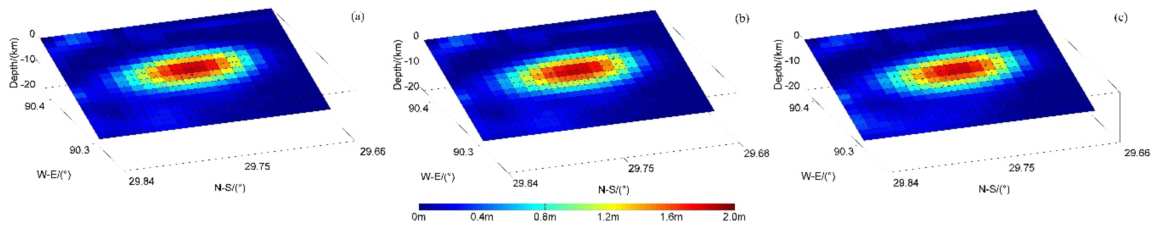
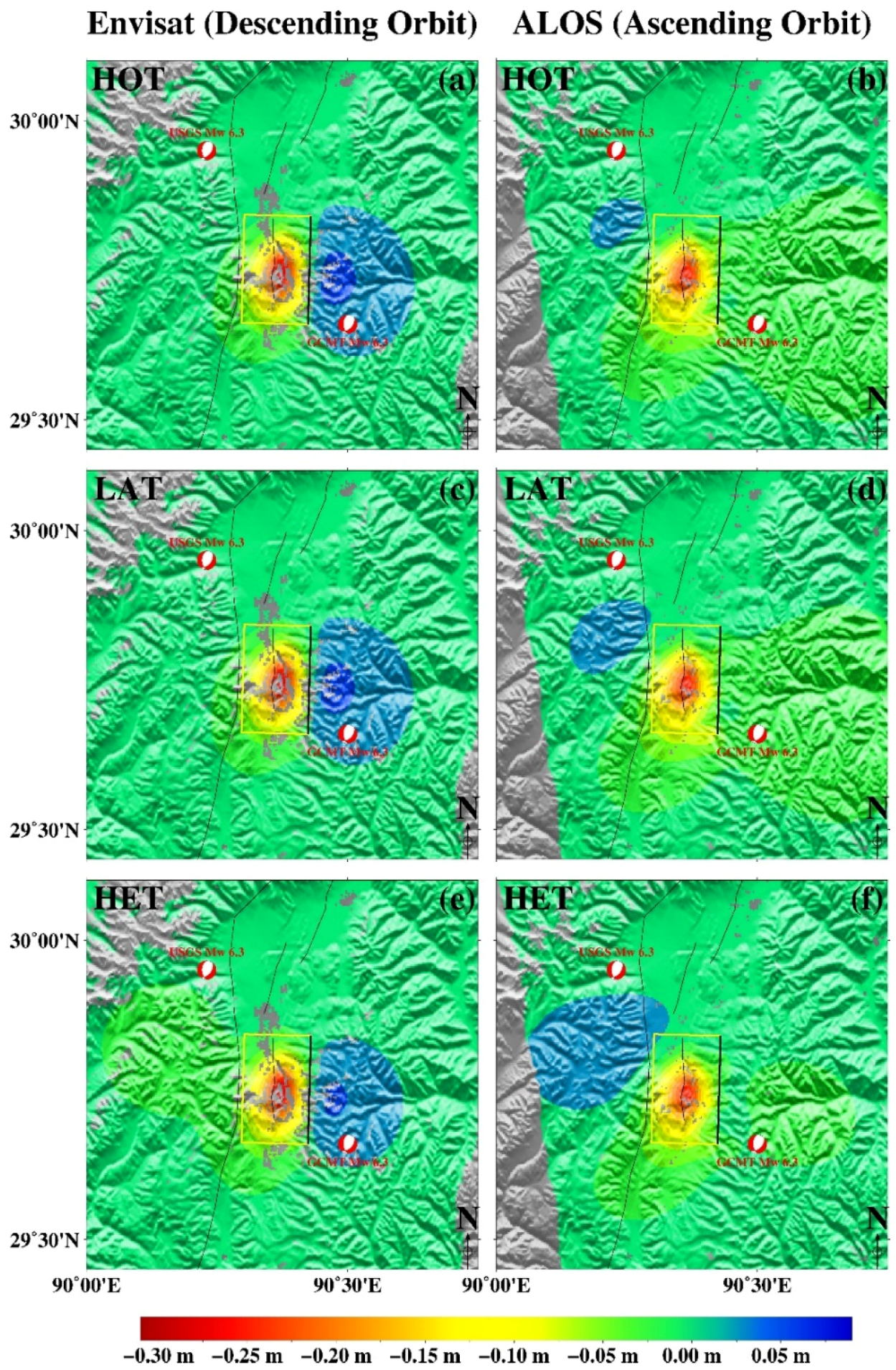
4.2. Comparison between Finite Element Models with Different Configurations

The residuals for the descending dataset from the HOT and LAT models indicate that, depending on the terms of goodness of fit, the discrepancies between the HOT model and the LAT model are barely detectible by the InSAR data for this earthquake. For a better understanding of the effect of the rigid crustal layering on slip distribution estimation, we examined the differences between the slip distribution estimated by the HOT model and the LAT model (Figure 14a). The differences are barely visible and are mainly distributed along the border of the main slip zone. These could be due to the coseismic slip being completely buried in the upper crust and the lower crust layer having little impact on the coseismic slip.
The resulting slip distribution for the HET model is shown in Figure 11c and Figure A1 where the maximum slip is about 1.99 m. Although the differences between the maximum slip movements of the HET and LAT models are small, the slip distribution of the HET model extends along the dip direction (Figure 14b). This could be caused by the relative stiffness between the hanging wall and footwall whereby the hanging wall is stiffer compared to the Miocene volcanic rocks but less stiff on the footwall relative to the granite [19,23,24]. Furthermore, the total geodetic moment of 3.5 × 10¹⁸ N·m estimated from the HET model is smaller than that of 3.53 × 10¹⁸ N·m estimated from the LAT model. The surface displacement for a given dislocation can be amplified by weak crustal material; the material properties of the HET model derived from previous methods are weaker than those of the LAT model, especially the material properties of the footwall in the HET model. The predicted coseismic deformations for the descending and ascending datasets in the LOS are shown in Figure 12; the root mean square misfits are reduced to 0.82 and 2.07 cm for the LAT model, and 0.82 and 1.96 cm for the HET model, respectively (Figure 12 and Figure 13).

4.3. Comparison with Other Slip Models

Although the main slip pattern derived from the HET model is similar to that shown in previous works [31,64,65,66,67], HET presents a wider estimated slip distribution than the slip distributions estimated from the previous works. Although the same data and fault geometry are adopted by the HET model and the analytical model of Liu et al., the slip estimated from the HET model is shallow, between 4.2 km and 11.1 km deep. However, the slip distribution estimated by the Okada model is concentrated at depths of 4.5–11 km [31]. Such a result indicates that the slip estimated by the FEMs is more widely distributed over the shallow portion of the surface rupture, whereas the estimated slip of the Okada model is more focused in the up-dip direction of the epicenter. The peak slip and the center of the main slip occur at a depth of approximately 7.1 km, which is shallower compared with the depth estimates of 7.5 km by Liu et al. [31], 10.95 km by Feng et al. [34], and 9.5 km estimated by Qiao et al. [67]. However, they are deeper than the 5-km depth derived by Sun et al. [65]; this last result can be attributed to their new method that assumes a uniform stress drop over the slip area of the fault to simultaneously invert for fault slip and fault geometry. The maximum slips calculated by the models of Liu et al. [31] and Qiao et al. [67] are 2.15 m and 3 m, respectively, which are larger than the maximum slip of 1.99 m of the HET model, while the 1.33-m maximum slip of Sun et al. [65] is smaller than our results. For the HOT model, the maximum slip is 2.05 m which is slightly smaller than Liu et al.’s result [31] showing a peak slip of 2.15 m possibly due to the effect of the topography. The estimated geodetic moment of the HET model in the research is 3.5 × 10¹⁸ N·m (MW 6.3), which is consistent with all the previous results [31,64,65,66,67].

4.4. Seismogenic Structure Background

Laboratory measurements indicate that the Young’s modulus of granite is between 2.6 × 10¹⁰ Pa and 6.9 × 10¹⁰ Pa, and the Young’s modulus of the Miocene volcanic rocks is between 2.0 × 10¹⁰ Pa and 9.8 × 10¹⁰ Pa [68]. Using the FEM inversion method, the optimal Young’s modulus values on the eastern and western sides of the fault are 2.6 × 10¹⁰ Pa and 7.8 × 10¹⁰ Pa, respectively. Our results show that the crustal parameters estimated from the inversion are consistent with those of a previous field survey that showed that the Yangyi basin is bordered by Paleogene granites to the east and by Miocene volcanic rock to the west [26]. Young’s modulus is the ratio of stress to strain, and so a stiff material needs more force to deform compared to a soft material. Our inverted results show that the Young’s modulus on the eastern side of the fault is much smaller than that in the west. Therefore, the 2008 Dangxiong event may have been induced by the different deformational rates caused by the E–W trending extension of southern Tibet [26].

4.5. Implications of this Study

We constructed FEMs of the 2008 Dangxiong earthquake to take account of the effect of the topography and medium heterogeneities. Although the discrepancies of the slip distributions and the root mean square which are estimated from the HOT model, LAT model and HET model are not evident, the HET model is much more realistic than the HOT model and the LAT model. As the HET model can account for topographic effects, crustal rigidity layering and medium heterogeneities, the systematic errors of these factors can be eliminated or reduced. By comparing the fit residuals’ distribution of the three FEMs (the HOT model, the LAT model, and the HET model), the area of the fit residuals has obviously been reduced, which confirms that the slip distribution estimated from the HET model can indeed fit better with the observations (Figure 12 and Figure 13). Thus, the effect of the topography and medium heterogeneities should not be ignored in elaborate models of earthquakes. Moreover, the medium heterogeneities which mainly refer to the estimation of the Young’s modulus in this work can be learned by the finite element method.

5. Conclusions

In this study, we mapped the coseismic deformation of the 2008 Dangxiong earthquake with Envisat ASAR C-band descending Track 176 and ALOS PALSAR L-band ascending Track 500 images without other geodetic data. The coseismic deformation pattern revealed by the InSAR observations confirmed that the deformation is concentrated mainly in a small region across the fault. We then constructed a geodetic FEM of the 2008 event to overcome the limitations of elastic homogeneity and the absence of topography. The forward modeling predictions using the FEMs indicate that the effects of various material parameters on the coseismic surface displacements are different. The coseismic surface displacements were more sensitive to variations in Young’s modulus than to variations in the topography or Poisson’s ratio as the topographic relief and the variations of Poisson’s ratio were small. Although the topographic relief in the Yadong–Gulu rift is large, it is relatively flat in the deformation region of the Dangxiong earthquake in Yangyi basin.
Based on our modelling, we used the FEMs to generate synthetic Green’s functions for static displacement; the linear inversion results provided a detailed description of the slip distribution of the Dangxiong earthquake. Taking into account the effect of lateral variations, we set constant values of Poisson’s ratio and density and changed the Young’s modulus on the eastern and western sides of the fault from 2 × 10¹⁰ Pa to 11 × 1010 Pa in 1 × 10⁹ Pa increments to search for the best fit model. The result indicates that when the Young’s modulus on the eastern side and western side of the fault are 2.6 × 10¹⁰ Pa and 7.8 × 10¹⁰ Pa, respectively, the model best fits the observations, which is consistent with a previous field survey. By comparing the slip distributions estimated from FEMs with different configurations and results of previous work, we reveal the differences and relationship among them: the slip distribution estimated from the HOT model is similar to that estimated from a homogeneous elastic half-space model; the discrepancies between the HOT model and the LAT model are barely detectible by the InSAR observations for this earthquake; the HET model can best fit the observations as it accounts for the effect of lateral variations. We also inverted the InSAR observations from two deformation profiles to estimate the Young’s modulus.

Acknowledgments

This work was financially supported by the National Natural Science Foundation of China (key program) under Grants No. 41431069, the Chinese 973 Program under Grants No. 2013CB733303 and 2013CB733304, the National Natural Science Foundation of China under Grants No. 41404007 and 41204010, and China National Special Fund for Earthquake Scientific Research in Public Interest under Grants No. 201308009. The Envisat ASAR data were supplied by ESA through the CAT-1 project (ID: 7195), and the ALOS PALSAR data were provided by JAXA through the RA3 project (ID: 608).

Author Contributions

Caijun Xu led the research and proposed the idea and structure of this manuscript. Bei Xu contributed to the conception of the study, performed the data analysis and wrote the paper. Caijun Xu, Yangmao Wen, and Yang Liu reviewed and edited the manuscript.

Conflicts of Interest

The authors declare no conflict of interest.

Appendix

Slip distribution estimated from the HET model.
Figure A1. Slip distributions estimated from the HET model with the DInSAR observations. Color scale shows slip movement in m.
Remotesensing 08 00228 g015

References

  1. Nikolaidis, R. Observation of Geodetic and Seismic Deformation with the Global Positioning System. Available online: http://sopac.ucsd.edu/input/processing/pubs/nikoThesis.pdf (accessed on 23 October 2015).
  2. Massonnet, D.; Feigl, K.L. Discrimination of geophysical phenomena in satellite radar interferograms. Geophys. Res. Lett. 1995, 22, 1537–1540. [Google Scholar] [CrossRef]
  3. Steketee, J.A. On Volterra’s dislocations in a semi-infinite elastic medium. Can. J. Phys. 1958, 36, 192–205. [Google Scholar] [CrossRef]
  4. Okada, Y. Surface deformation due to shear and tensile faults in a half-space. B Seismol. Soc. Am. 1985, 75, 1135–1154. [Google Scholar]
  5. Bonafede, M.; Parenti, B.; Rivalta, E. On strike-slip faulting in layered media. Geopys. J. Int. 2002, 149, 698–723. [Google Scholar] [CrossRef]
  6. Fernández, J.; Yu, T.T.; Rundle, J.B. Horizontal viscoelastic-gravitational displacement due to a rectangular dipping thrust fault in a layered Earth model. J. Geophys. Res. 1996, 101, 13581–13594. [Google Scholar] [CrossRef]
  7. Megna, A.; Barba, S.; Santini, S.; Dragoni, M. Effects of geological complexities on coseismic displacement: Hints from 2D numerical modelling. Terra Nova 2008, 20, 173–179. [Google Scholar] [CrossRef] [Green Version]
  8. Zhao, S.; Müller, R.D.; Takahashi, Y.; Kaneda, Y. 3-D finite-element modelling of deformation and stress associated with faulting: Effect of inhomogeneous crustal structures. Geopys. J. Int. 2004, 157, 629–644. [Google Scholar] [CrossRef]
  9. Williams, C.A.; Wadge, G. An accurate and efficient method for including the effects of topography in three-dimensional elastic models of ground deformation with applications to radar interferometry. J. Geophys. Res. 2000, 105, 8103–8120. [Google Scholar] [CrossRef]
  10. Bonafede, M.; Rivalta, E. On tensile cracks close to and across the interface between two welded elastic half-spaces. Geopys. J. Int. 1999, 138, 410–434. [Google Scholar] [CrossRef]
  11. Taira, A.; Saito, S.; Aoike, K.A.N.; Morita, S.; Tokuyama, H.; Suyehiro, K.; Klaus, A. Nature and growth rate of the Northern Izu–Bonin (Ogasawara) arc crust and their implications for continental crust formation. Isl. Arc 1998, 7, 395–407. [Google Scholar] [CrossRef]
  12. Iwasaki, T.; Kato, W.; Moriya, T.; Hasemi, A.; Umino, N.; Okada, T.; Miyamachi, H. Extensional structure in Northern Honshu Arc as inferred from seismic refraction/wide-angle reflection profiling. Geophys. Res. Lett. 2001, 28, 2329–2332. [Google Scholar] [CrossRef]
  13. Du, Y.; Segall, P.; Gao, H. Dislocations in inhomogeneous media via a moduli perturbation approach: General formulation and two-dimensional solutions. J. Geophys. Res. Sol. Earth 1994, 99, 13767–13779. [Google Scholar] [CrossRef]
  14. Simons, M.; Fialko, Y.; Rivera, L. Coseismic deformation from the 1999 Mw 7.1 Hector Mine, California, earthquake as inferred from InSAR and GPS observations. B Seismol. Soc. Am. 2002, 92, 1390–1402. [Google Scholar] [CrossRef]
  15. Hearn, E.H.; Bürgmann, R. The effect of elastic layering on inversions of GPS data for coseismic slip and resulting stress changes: Strike-slip earthquakes. B Seismol. Soc. Am. 2005, 95, 1637–1653. [Google Scholar] [CrossRef]
  16. Sato, K.; Minagawa, N.; Hyodo, M.; Baba, T.; Hori, T.; Kaneda, Y. Effect of elastic inhomogeneity on the surface displacements in the northeastern Japan: Based on three-dimensional numerical modeling. Earth Planets Space 2007, 59, 1083–1093. [Google Scholar] [CrossRef]
  17. Masterlark, T.; Hughes, K.L. Next generation of deformation models for the 2004 M9 Sumatra-Andaman earthquake. Geophys. Res. Lett. 2008, 35. [Google Scholar] [CrossRef]
  18. Xu, B.; Xu, C. Numerical simulation of influences of the earth medium’s lateral heterogeneity on co-and post-seismic deformation. Geodesy Geodyn. 2015, 6, 46–54. [Google Scholar] [CrossRef]
  19. Masterlark, T. Finite element model predictions of static deformation from dislocation sources in a subduction zone: Sensitivities to homogeneous, isotropic, Poisson-solid, and half-space assumptions. J. Geophys. Res. 2003, 108. [Google Scholar] [CrossRef]
  20. Dubois, L.; Feigl, K.L.; Komatitsch, D.; Árnadóttir, T.; Sigmundsson, F. Three-dimensional mechanical models for the June 2000 earthquake sequence in the south Iceland seismic zone. Tectonophysics 2008, 457, 12–29. [Google Scholar] [CrossRef]
  21. Moreno, M.S.; Bolte, J.; Klotz, J.; Melnick, D. Impact of megathrust geometry on inversion of coseismic slip from geodetic data: Application to the 1960 Chile earthquake. Geophys. Res. Lett. 2009, 36. [Google Scholar] [CrossRef]
  22. Currenti, G.; Bonaccorso, A.; Del Negro, C.; Guglielmino, F.; Scandura, D.; Boschi, E. FEM-based inversion for heterogeneous fault mechanisms: Application at Etna volcano by DInSAR data. Geopys. J. Int. 2010, 183, 765–773. [Google Scholar] [CrossRef]
  23. Hsu, Y.J.; Simons, M.; Williams, C.; Casarotti, E. Three-dimensional FEM derived elastic Green’s functions for the coseismic deformation of the 2005 Mw 8.7 Nias-Simeulue, Sumatra earthquake. Geochem. Geophys. Geosyst. 2011, 12. [Google Scholar] [CrossRef]
  24. Trasatti, E.; Kyriakopoulos, C.; Chini, M. Finite element inversion of DInSAR data from the Mw 6.3 L’Aquila earthquake, 2009 (Italy). Geophys. Res. Lett. 2011, 38. [Google Scholar] [CrossRef]
  25. Tizzani, P.; Castaldo, R.; Solaro, G.; Pepe, S.; Bonano, M.; Casu, F.; Lanari, R. New insights into the 2012 Emilia (Italy) seismic sequence through advanced numerical modeling of ground deformation InSAR measurements. Geophys. Res. Lett. 2013, 40, 1971–1977. [Google Scholar] [CrossRef]
  26. Wu, Z.H.; Ye, P.S.; Barosh, P.J.; Wu, Z.H. The 6 October 2008 MW 6.3 magnitude Damxung earthquake, Yadong-Gulu rift, Tibet, and implications for present-day crustal deformation within Tibet. J. Asian Earth Sci. 2011, 40, 943–957. [Google Scholar] [CrossRef]
  27. Chen, Q.; Freymueller, J.T.; Wang, Q.; Yang, Z.; Xu, C.; Liu, J. A deforming block model for the present-day tectonics of Tibet. J. Geophys. Res. 2004, 109. [Google Scholar] [CrossRef]
  28. Chen, Q.; Freymueller, J.T.; Yang, Z.; Xu, C.; Jiang, W.; Wang, Q.; Liu, J. Spatially variable extension in southern Tibet based on GPS measurements. J. Geophys. Res. 2004, 9. [Google Scholar] [CrossRef]
  29. Earthquake Disaster Prevention Department of China Earthquake Administration (EDPD-CEA). Catalogue of Historical Earthquakes in China; Earthquake Press: Beijing, China, 1995. (In Chinese) [Google Scholar]
  30. Earthquake Disaster Prevention Department of China Earthquake Administration (EDPD-CEA). Catalogue of Historical Earthquakes in China; Earthquake Press: Beijing, China, 1999. (In Chinese) [Google Scholar]
  31. Liu, Y.; Xu, C.; Wen, Y.; He, P.; Jiang, G. Fault rupture model of the 2008 Dangxiong (Tibet, China) MW 6.3 earthquake from Envisat and ALOS data. Adv. Space Res. 2012, 50, 952–962. [Google Scholar] [CrossRef]
  32. Gan, W.; Zhang, P.; Shen, Z.K.; Niu, Z.; Wang, M.; Wan, Y.; Cheng, J. Present-day crustal motion within the Tibetan Plateau inferred from GPS measurements. J. Geophys. Res. 2007, 112. [Google Scholar] [CrossRef]
  33. Armijo, R.; Tapponnier, P.; Mercier, J.L.; Han, T.L. Quaternary extension in southern Tibet: Field observations and tectonic implications. J. Geophys. Res. 1986, 91, 13803–13872. [Google Scholar] [CrossRef]
  34. Feng, W.; Xu, L.; Li, Z. Fault parameters of the October 2008 Damxung MW 6.3 earthquake from InSAR inversion and its tectonic implication. Chin. J. Geophys. 2010, 53, 1134–1142. (In Chinese) [Google Scholar]
  35. Peltzer, G.; Saucier, F. Present-day kinematics of Asia derived from geologic fault rates. J. Geophys. Res. 1996, 101, 27943–27956. [Google Scholar] [CrossRef]
  36. Deng, Q.; Zhang, P.; Ran, Y.; Yang, X.; Min, W.; Chu, Q. Basic characteristics of active tectonics of China. Sci. China Ser. D 2003, 46, 356–372. [Google Scholar]
  37. Fialko, Y.; Simons, M.; Agnew, D. The complete (3-D) surface displacement field in the epicentral area of the 1999 Mw 7.1 Hector Mine Earthquake, California, from space geodetic observations. Geophys. Res. Lett. 2001, 28, 3063–3066. [Google Scholar] [CrossRef]
  38. Fialko, Y. Probing the mechanical properties of seismically active crust with space geodesy: Study of the coseismic deformation due to the 1992 Mw 7.3 Landers (southern California) earthquake. J. Geophys. Res. 2004, 109. [Google Scholar] [CrossRef]
  39. Rosen, P.A.; Hensley, S.; Peltzer, G.; Simons, M. Updated repeat orbit interferometry package released. Eos Trans. Am. Geophys. Union 2004, 85, 47. [Google Scholar] [CrossRef]
  40. Goldstein, R.M.; Werner, C.L. Radar interferogram filtering for geophysical applications. Geophys. Res. Lett. 1998, 25, 4035–4038. [Google Scholar] [CrossRef]
  41. Goldstein, R.; Zebker, H.; Werner, C. Satellite radar interferometry-Two-dimensional phase unwrapping. Radio Sci. 1988, 23, 713–720. [Google Scholar] [CrossRef]
  42. Hanssen, R.F. Radar Interferometry: Data Interpretation and Error Analysis, 1st ed.; Kluwer Academic Publishers: Dordrecht, The Netherlands, 2001. [Google Scholar]
  43. Gable, C.W.; Trease, H.E.; Cherry, T.A. Geological Applications of Automatic Grid Generation Tools for Finite Elements Applied to Porous Flow Modeling. In Numerical Grid Generation in Computational Fluid Dynamics and Related Fields; Mississippi State University Press: Jackson, MS, USA, 1996; pp. 1–9. [Google Scholar]
  44. Aagaard, B.; Kientz, S.; Knepley, M.G.; Somala, S.; Strand, L.; Williams, C. PyLith User Manual, Version 1.7.1, Computational Infrastructure for Geodynamics (CIG), University of California, Davis, Calif. 2012; Available online: http://www.geodynamics.org/cig/software/pylith/pylith_manual-1.7.1.pdf (accessed on 6 May 2013).
  45. Farr, T.G.; Rosen, P.A.; Caro, E.; Crippen, R.; Duren, R.; Hensley, S.; Alsdorf, D. The shuttle radar topography mission. Rev. Geophys. 2007, 45. [Google Scholar] [CrossRef]
  46. Melosh, H.J.; Raefsky, A. A simple and efficient method for introducing faults into finite element computations. B Seismol. Soc. Am. 1981, 71, 1391–1400. [Google Scholar] [CrossRef]
  47. Laske, G.; Masters, G.; Ma, Z.; Pasyanos, M. Update on CRUST1. 0-A 1-degree global model of Earth’s crust. Geophys. Res. Abstr. 2013, 15, 2658. [Google Scholar]
  48. Xu, C.; Liu, Y.; Wen, Y.; Wang, R. Coseismic slip distribution of the 2008 MW 7.9 Wenchuan earthquake from joint inversion of GPS and InSAR data. B Seismol. Soc. Am. 2010, 100, 2736–2749. [Google Scholar] [CrossRef]
  49. Du, Y.; Aydin, A.; Segall, P. Comparison of various inversion techniques as applied to the determination of a geophysical deformation model for the 1983 Borah Peak earthquake. B Seismol. Soc. Am. 1992, 82, 1840–1866. [Google Scholar]
  50. Freymueller, J.; King, N.E.; Segall, P. The co-seismic slip distribution of the Landers earthquake. B Seismol. Soc. Am. 1994, 84, 646–659. [Google Scholar]
  51. Jónsson, S.; Zebker, H.; Segall, P.; Amelung, F. Fault slip distribution of the 1999 Mw 7.1 Hector Mine, California, earthquake, estimated from satellite radar and GPS measurements. B Seismol. Soc. Am. 2002, 92, 1377–1389. [Google Scholar] [CrossRef]
  52. Hansen, P.C. Rank-Deficient and Discrete Ill-Posed Problems: Numerical Aspects of Linear Inversion; Siam: Philadelphia, PA, USA, 1998; Volume 4, pp. 1–206. [Google Scholar]
  53. Tinti, S.; Armigliato, A. A 2-D hybrid technique to model the effect of topography on coseismic displacements. Application to the Umbria-Marche (central Italy) 1997 earthquake sequence. Geophys. J. Int. 2002, 150, 542–557. [Google Scholar] [CrossRef]
  54. Wang, K.; He, J. Mechanics of low-stress forearcs: Nankai and Cascadia. J. Geophys. Res. 1999, 104, 15191–15205. [Google Scholar] [CrossRef]
  55. Christensen, N.I. Poisson’s ratio and crustal seismology. J. Geophys. Res. 1996, 101, 3139–3156. [Google Scholar] [CrossRef]
  56. Vauchez, A.; Tommasi, A.; Barruol, G. Rheological heterogeneity, mechanical anisotropy and deformation of the continental lithosphere. Tectonophysics 1998, 296, 61–86. [Google Scholar] [CrossRef] [Green Version]
  57. Russo, R.M.; Silver, P.G. Trench-parallel flow beneath the Nazca plate from seismic anisotropy. Science 1994, 263, 1105–1111. [Google Scholar] [CrossRef] [PubMed]
  58. Yang, X.; Fischer, K.M.; Abers, G.A. Seismic anisotropy beneath the Shumagin Islands segment of the Aleutian-Alaska subduction zone. J. Geophys. Res. 1995, 100, 18165–18177. [Google Scholar] [CrossRef]
  59. Ismail, W.B.; Mainprice, D. An olivine fabric database: An overview of upper mantle fabrics and seismic anisotropy. Tectonophysics 1998, 296, 145–157. [Google Scholar] [CrossRef]
  60. Godfrey, N.J.; Christensen, N.I.; Okaya, D.A. Anisotropy of schists: Contribution of crustal anisotropy to active source seismic experiments and shear wave splitting observations. J. Geophys. Res. 2000, 105, 27991–28007. [Google Scholar] [CrossRef]
  61. Masterlark, T.; DeMets, C.; Wang, H.F.; Sanchez, O.; Stock, J. Homogeneous vs. heterogeneous subduction zone models: Coseismic and postseismic deformation. Geophys. Res. Lett. 2001, 28, 4047–4050. [Google Scholar] [CrossRef]
  62. Kern, H.; Richter, A. Temperature derivatives of compressional and shear-wave velocities in crustal and mantle rocks at 6 kbar confining pressure. J. Geophys. Z. Geophys. 1981, 49, 47–56. [Google Scholar]
  63. Beaumont, C.; Jamieson, R.A.; Nguyen, M.H.; Lee, B. Himalayan tectonics explained by extrusion of a low-viscosity crustal channel coupled to focused surface denudation. Nature 2001, 414, 738–742. [Google Scholar] [CrossRef] [PubMed]
  64. Bie, L.; Ryder, I.; Nippress, S.E.; Bürgmann, R. Coseismic and post-seismic activity associated with the 2008 Mw 6.3 Damxung earthquake, Tibet, constrained by InSAR. Geophys. J. Int. 2014, 196, 788–803. [Google Scholar] [CrossRef]
  65. Sun, J.; Johnson, K.M.; Cao, Z.; Shen, Z.; Bürgmann, R.; Xu, X. Mechanical constraints on inversion of coseismic geodetic data for fault slip and geometry: Example from InSAR observation of the 6 October 2008 MW 6.3 Dangxiong-Yangyi (Tibet) earthquake. J. Geophys. Res. 2011, 116, B1. [Google Scholar] [CrossRef]
  66. Elliott, J.R.; Walters, R.J.; England, P.C.; Jackson, J.A.; Li, Z.; Parsons, B. Extension on the Tibetan plateau: Recent normal faulting measured by InSAR and body wave seismology. Geophys. J. Int. 2010, 183, 503–535. [Google Scholar] [CrossRef]
  67. Qiao, X.; You, X.; Yang, S.; Wang, Q.; Wang, R. Study on dislocation inversion of MS 6.6 Damxung earthquake as constrained by InSAR measurement. J. Geod. Geodyn. 2009, 2009, 1–7. (In Chinese) [Google Scholar]
  68. Jaeger, J.C.; Cook, N.G.; Zimmerman, R. Fundamentals of Rock Mechanics, 4th ed.; Blackwell Publishing: Oxford, UK, 2007; pp. 1–488. [Google Scholar]
Figure 1. Tectonic setting of the 6 October 2008 Dangxiong MW 6.3 earthquake. Location of study area on the globe, and map of study area with major tectonic faults [35]. Black rectangles mark the areas covered by the Envisat ASAR (Descending Track 176) and ALOS PALSAR SAR data (Ascending Track 500); AZI and LOS refer to satellite azimuth and look direction, respectively. Light blue box denotes the fault surface projection on the ground with the black line as its top. Thin black lines denote the Quaternary active faults [36]. Red beach balls represent the earthquake source mechanisms (from USGS and GCMT). Gray solid circles indicate the location of aftershocks. Black solid circles with the time and magnitude indicate historic earthquake events [29,30].
Remotesensing 08 00228 g001
Figure 2. Coseismic deformation of the 6 October 2008 MW 6.3 Dangxiong earthquake along the Line Of Sight (LOS) observed by Envisat ASAR and ALOS PALSAR. (a) The descending orbit interferogram observed by Envisat ASAR; (b) The ascending orbit interferogram observed by ALOS PALSAR. Yellow box denotes the fault surface projection on the ground with the black line as its top. Thin black lines denote the Quaternary active faults [36]. Red beach balls represent the earthquake source mechanisms (from USGS and GCMT).
Remotesensing 08 00228 g002
Figure 3. The FEMs of the 6 October 2008 MW 6.3 Dangxiong earthquake. The fault of the Dangxiong earthquake embedded into 3-D FEM with a flat surface and a dimension of 200 × 200 × 310 km. Black solid line located at the junction of the two mediums indicate the location of the fault.
Remotesensing 08 00228 g003
Figure 4. FEM of the Dangxiong earthquake deformation region with realistic topographic relief surface.
Remotesensing 08 00228 g004
Figure 5. The flow chart of the procedure for solving the inverse problem of the earthquake fault mechanism.
Remotesensing 08 00228 g005
Figure 6. Contour maps of coseismic surface displacements and differences between the flat free surface model and the topographic relief model. The contour interval is shown at the bottom left corner. (a) Horizontal coseismic surface displacements estimated from the model with topographic relief; (b) Differences between horizontal displacements of the model with flat free surface and the model with topographic relief; (c) Vertical coseismic surface displacements estimated from the model with topographic relief; (d) Differences between vertical displacements of the model with flat free surface and the model with topographic relief.
Remotesensing 08 00228 g006
Figure 7. Contour maps of coseismic surface displacements and differences between models with Poisson’s ratio of 0.25 and 0.3. The contour interval is shown at the bottom left corner. (a) Horizontal coseismic surface displacements estimated from the model with Poisson’s ratio of 0.25; (b) Differences between horizontal displacements of models with Poisson’s ratio of 0.25 and 0.3; (c) Vertical coseismic surface displacements estimated from the model with Poisson’s ratio of 0.25; (d) Differences between vertical displacements of models with Poisson’s ratio of 0.25 and 0.3.
Remotesensing 08 00228 g007
Figure 8. Contour map of coseismic surface displacements and differences between models with Young’s modulus of 9 × 10¹⁰ Pa and 4 × 10¹⁰ Pa. The contour interval is shown at the left bottom corner. (a) Horizontal coseismic surface displacement estimated from the model with Young’s modulus of 4 × 10¹⁰ Pa; (b) Differences in horizontal displacements between models with Young’s modulus of 9 × 10¹⁰ Pa and 4 × 10¹⁰ Pa; (c) Vertical coseismic surface displacement estimated from model with Young’s modulus of 4 × 10¹⁰ Pa; (d) Differences in vertical displacements between models with Young’s modulus of 9 × 10¹⁰ Pa and 4 × 10¹⁰ Pa.
Remotesensing 08 00228 g008
Figure 9. Trade-off curves of three models between the weighted misfit and the roughness.
Remotesensing 08 00228 g009
Figure 10. Weighted misfits estimated from the same smoothing factor of κ2 = 0.05. The red circle represents the smallest weighted misfits.
Remotesensing 08 00228 g010
Figure 11. Slip distributions inferred from the DInSAR observations. Panels (a); (b); and (c) correspond to the HOmogeneous with Topography (HOT) model, the LAyering with Topography (LAT) model, and the HEterogeneous with Topography (HET) model, respectively. Color scale shows slip movement in m.
Remotesensing 08 00228 g011
Figure 12. Predicted coseismic deformation for the descending and ascending datasets in LOS. (a,c,e) Envisat ASAR Track 176 estimated by the HOT, LAT, and HET models , respectively; (b,d,f) ALOS PALSAR Track 500 estimated by the HOT model, LAT model, and HET model, respectively. Yellow box denotes the fault surface projection on the ground with the black line as its top. Thin black lines denote the Quaternary active faults [36]. Red beach balls represent the earthquake source mechanisms (from USGS and GCMT).
Remotesensing 08 00228 g012
Figure 13. Fit residuals for descending and ascending datasets in LOS. (a,c,e) Envisat ASAR Track 176 estimated by the HOT model, LAT model, and HET model, respectively; (b,d,f) ALOS PALSAR Track 500 estimated by the HOT model, LAT model, and HET model, respectively. Yellow box denotes the fault surface projection on the ground with the black line as its top. Thin black lines denote the Quaternary active faults [36]. Red beach balls represent the earthquake source mechanisms (from USGS and GCMT).
Remotesensing 08 00228 g013
Figure 14. Difference of coseismic slip distribution. (a) Difference between HOT and LAT (Diff = HOT − LAT); (b) Difference between HET and LAT (Diff = HET − LAT).
Remotesensing 08 00228 g014
Table 1. SAR satellite data used in this work.
SatelliteDate1 yymmddDate2 yymmddBperp a mTrack (A/D) bσ c cml d kmFrom
Envisat0704150904190.47176(D)0.438.6Liu et al. [31]
ALOS070213090821−72.5500(A)1.535.3
a Perpendicular baseline at the scene center; b A denotes ascending track, and D descending track; c Standard deviation of the interferogram’s noise; d e-folding spatial scale of the interferogram’s 1D covariance function, calculated using data from the interferogram with masked out within area of epicenter [42].
Table 2. Fault rupture parameters of the 6 October 2008 Dangxiong MW 6.3 earthquake.
Strike (°)Dip (°)Rake (°)Slip mLongitude a (°)Latitude a (°)Length kmWidth b kmTop c kmFrom
182.1854.36variablevariable90.426729.749820200Liu et al. [31]
a Center point (Longitude and Latitude) of the fault plane projected to the earth surface; b Width of the fault plane in dipping direction; c Minimum depth of the fault plane.
Table 3. Continental crust configuration from the Crust 1.0 model.
LayersThickness kmρ kg/m3Vs m/sVp m/s
upper crust382720.03520.06000.0
middle crust182790.03680.06300.0
lower crust202850.03820.06600.0

