Stereoscopic Estimation of Volcanic Ash Cloud-Top Height from Two Geostationary Satellites

Abstract

The characterization of volcanic ash clouds released into the atmosphere during explosive eruptions includes cloud height as a fundamental physical parameter. A novel application is proposed of a method based on parallax data acquired from two geostationary instruments for estimating ash cloud-top height (ACTH). An improved version of the method with a detailed discussion of height retrieval accuracy was applied to estimate ACTH from two datasets acquired by two satellites in favorable positions to fully exploit the parallax effect. A combination of MSG SEVIRI (HRV band; 1000 m nadir spatial resolution, 5 min temporal resolution) and Meteosat-7 MVIRI (VIS band, 2500 m nadir spatial resolution, 30 min temporal resolution) was implemented. Since MVIRI does not acquire data at exactly the same time as SEVIRI, a correction procedure enables compensation for wind advection in the atmosphere. The method was applied to the Mt. Etna, Sicily, Italy, eruption of 23 November 2013. The height of the volcanic cloud was tracked with a top height of ~8.5 km. The ash cloud estimate was applied to the visible channels to show the potential accuracy that will soon be achievable also in the infrared range using the next generation of multispectral imagers. The new constellation of geostationary meteorological satellites will enable full exploitation of this technique for continuous global ACTH monitoring.

1. Introduction

An estimation of ash cloud-top height (ACTH) affects estimation of cloud location, the resulting height of the most dangerous zone for air traffic, the forecast accuracy of transport and deposition models [1], the quantitative retrieval of the ash cloud burden [2,3,4], the estimation of mass eruption rate [5,6], etc. Many techniques have been proposed to measure the volcanic ACTH from ground-based instruments, including those based on ground weather radar [7,8,9] and volcano surveillance cameras [10]. These methods typically offer very accurate estimates of the height of the eruption column, but are only applicable to a few better-monitored volcanoes. Continuous ACTH measurements of volcanic ash layers can also be obtained from ground-based LiDARs, either near the volcano source where these instruments are deployed [11], or on the nodes of ceilometer and LiDAR networks [12,13,14,15].

Satellite data offers the best way to extend the ability to estimate ACTH when volcanic eruptions occur, providing the continuous global coverage required for effective monitoring [16].

Table 1. Overview of satellite methods for cloud top height retrieval.

Methodology	Pros/Cons
LiDAR and radar [6,19,24]	+ very high vertical resolution and accuracy – excessive revisit time (16 days) and only nadir observations from currently-operational instruments (LiDAR CALIOP, radar CPR)
Radio occultation [25,26]	+ high resolution in lower troposphere – globally available only about 2000 times per day
Backward trajectory modeling [27,28]	+ estimate possible even for clouds drifted away from the source – requires wind field data for a large area and a reliable trajectory model (e.g., turbulence not easy to handle); homogenous wind field results with high uncertainty of the source height
Brightness temperature [3,17,27]	+ easy to apply, possible with instruments with a short revisit time – requires atmospheric profile and emissivity of the cloud; assumption of thermal equilibrium; problems around tropopause
O2 A-band absorption [29]	+ high accuracy – requires high spectral resolution data (not available on many satellites, long revisit time); good performance only over dark surfaces; requires radiative transfer modeling; daytime only
CO2 absorption [21,30,31]	+ good performance also with semi-transparent clouds – accurate only in the high levels of the troposphere; problems around tropopause
Shadow length [3,32]	+ easy to apply; requires no additional data – possible only during daytime; retrieves the height of the cloud horizontal edge and not its top
Stereoscopy [17,23,33,34,35,36,37]	+ high accuracy; requires no additional data; based on geometry→no problems in the case of ash reaching the stratosphere – requires simultaneous data from two different viewpoints
Optimal estimation [38,39,40]	+ includes error estimate − requires atmospheric profiles, ash optical properties, and radiative transfer

briefly reviews quantitative satellite remote sensing techniques for ash/meteorological cloud height retrieval. The accuracy of the listed methods depends on the spatial resolution of the sensors and the cloud height [17]. The best estimates using LiDAR from a space-based platform offer an accuracy within less than 200 m, and can provide either daytime and night-time measurements of a volcanic cloud height and thickness with a revisit time of 16 days [18]. When available, ash cloud height measured by LiDARs or LiDAR networks are very valuable for comparison validation with other observations in integrated and synergistic approaches [6,19,20]. Operational height estimates based on CO₂ absorption [21] are available several times a day but with significantly lower accuracy [22]: bias = −1.4 km; std = 2.9 km. A recent method based on the parallax between volcanic ash cloud images recorded by the satellite multispectral sensors MODIS (Moderate Resolution Imaging Spectroradiometer) and SEVIRI (Spinning Enhanced Visible and InfraRed Imager) achieves a higher accuracy of ~600 m. It was developed and successfully applied to the large 2010 Eyjafjallajökull eruption by Zakšek et al. [23]. This method exploits the different points of view of the SEVIRI instrument on board the MSG geostationary platform, and the MODIS instrument on board the polar-orbiting AQUA and TERRA platforms, for the observation of volcanic ash clouds produced during eruptions. The use of these two sensors makes the most of the better spatial resolution of MODIS, but is conversely limited by only a few MODIS acquisition per day. Moreover, the position of MODIS changes continuously, reducing the number of MODIS and SEVIRI image couples of the same eruption that can be effectively used to estimate the height of a volcanic cloud.

The use of two sensors, both onboard geostationary platforms, would allow maximization of the number of pairs of images available for ACTH estimation, making it possible to follow the evolution of a volcanic ash cloud height. The current EUMETSAT policy for the use of geostationary weather satellites is to position the newest satellite in the best nominal position (0° longitude) with an Earth full-disk acquisition every 15 min, moving the previous satellite in a back-up position (9.5° E longitude) in rapid scan mode service (RSS) with acquisition focused on much of the northern hemisphere every 5 min.

Attempts to use pairs of images acquired by these two SEVIRI sensors to estimate the height of volcanic clouds have been unsuccessful because the baseline, i.e., the difference in angle of view between the two sensors, is too small and, consequently, the error in the estimated height is too large at the current spatial resolution of SEVIRI (1000 m in nadir for the HRV channel). However, one of the available satellites previously launched was subsequently moved by EUMETSAT to the position 57.5° E degrees over the Indian Ocean, supporting the Indian Ocean Data Coverage (IODC) service. The difference in angle of view of the IODC satellite relative to both the main satellite (0° longitude) and back-up satellite (9.5° E longitude) allows better exploitation of the parallax method for ACTH estimation.

Currently, the satellite located on the Indian Ocean is Meteosat First Generation (MFG) carrying aboard the Meteosat Visible and InfraRed Imager (MVIRI), which is the predecessor of SEVIRI. Although the characteristics of SEVIRI are superior to those of MVIRI, the data acquired by this pair of sensors can be exploited to illustrate the potential of the parallax method when applied to two sensors on geostationary platforms placed in optimal geometric positions [41]. The short term development plans of all the major space agencies include an increased number of meteorological geostationary platforms with multispectral sensors capable of capturing images with improved spatial and temporal resolution, such the Advanced Himawari Imager recently launched on platform HIMAWARI-8, the Flexible Combine Imager (FCI) on Meteosat Third Generation (MTG-I) platform in the Sentinel-4 mission, and the Advanced Baseline Imager (ABI) on the Geostationary Operational Environmental Satellite-R Series (GOES-R). The method developed and described in this article will then be able to provide even more accurate ACTH estimates.

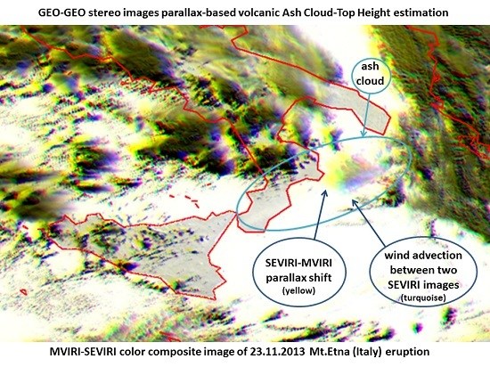
The next sections will describe the sensors and data used for the Mt. Etna (Sicily, Italy) eruption that occurred on 23 November 2013. This eruption was a short-lived lava fountain episode, and was chosen because it was short and difficult to characterize, therefore suitable to reveal any problems of the proposed approach. Moreover, clear sequences of images were captured by both SEVIRI and MVIRI (Section 2). The application and description of the parallax method (Section 3) refers to this selected Mt. Etna case study. The results are discussed in Section 4.

2. Datasets

Several details are crucial to correctly synchronize the stereo couples from two different sensors and improve the accuracy of ACTH estimation. The importance of precise geographic positioning and exact time determination for each pixel will be discussed in Section 3. However, it is first necessary to establish the exact position of the satellite itself. Although the satellites in question are called “geostationary”, in reality the projection of their orbit onto the Earth’s surface is not a single point but instead could be represented approximately as a number “8”. The position of each satellite can vary by several degrees from its nominal position; thus, it is necessary to determine the position as a function of time. Although such an orbit is not easy to parameterize, it can be closely approximated in a short period of time (about one hour) using a third-degree polynomial from the metadata provided in the EUMETSAT data product (level 1.5 in HDF format was applied for both products).

In order to exploit the spatial resolution of the two instruments to the maximum, the datasets used where the broad visible channels of both MVIRI (VIS 0.50–0.90 μm) and SEVIRI (HRV 0.6–0.9 μm). This choice offered the best possible ACTH estimation accuracy.

2.1. MVIRI

On the 5th of December 2006 EUMETSAT relocated the Meteosat-7 satellite over longitude 57.5° E for the IODC service. Meteosat-7 is the last operational unit of the Meteosat First Generation (MFG) program carrying aboard the MVIRI sensor. The satellite is spin-stabilized and the MVIRI data are acquired at the rate of one image line per satellite rotation. Thus, the Earth disk is scanned horizontally from east to west at each rotation and when the line is completed the next is collected with a stepping tilt mirror operated from south to north. At 100 rpm a whole image of 2500 scan lines is acquired every 25 min over IR (thermal infrared wavelengths in the range 10.5 to 12.5 μm) and WV (radiation from the water vapour absorption band in the range 5.70 to 7.10 µm) spectral bands. At the same time a third composite image is acquired in the visible to near infrared range (0.5 to 0.9 μm, VIS) by two detectors with a twice finer resolution than the IR and WV detectors. A 5 min retrace and stand-by period prepares the sensor for the next image acquisition and completes the 30 min repetition cycle of MVIRI, which is 48 data acquisitions per day. The full disk complete images are 2500 × 2500 8-bit pixels for the IR and WV bands, doubled resolution (5000 lines of 5000 pixels) for the VIS band, with a ground resolution at the sub-satellite point of 5 km for the IR and WV images, and 2.5 km for the VIS image.

2.2. SEVIRI

The primary instrument of the Meteosat Second Generation (MSG) is the SEVIRI radiometer characterized by 12 spectral channels from visible to thermal infrared and a repetition cycle of full disk acquisition of 15 min for a nominal satellite located at 0° longitude. The backup satellite located at 9.5° E is operated in rapid scan service mode (RSS) and provides one image of the northern part of the hemisphere every 5 min. The high-resolution visible channel (HRV) has a ground resolution of 1 km at nadir, while the other 11 channels have a resolution of 3 km.

The acquisition of SEVIRI is similar to MVIRI in that it exploits a 100 rpm counter-clockwise spin used to stabilize the satellite platform and to align its longitudinal rotation axis with the Earth’s rotational axis. However, MVIRI has a single detector per channel (two for the VIS channel) while SEVIRI has three detectors per channel scanning three lines simultaneously (nine for HRV), which results in larger images: 3712 × 3712 pixels (11,136 × 11,136 for HRV channel). Every repeat cycle of 15 min is required for a complete full disk image acquisition and transmission is composed of eight data image segments (24 segments for the HRV channel). Each segment has 464 lines of image data, with acquisition starting at the lower right pixel and ending at the top left pixel.

3. The Parallax Method

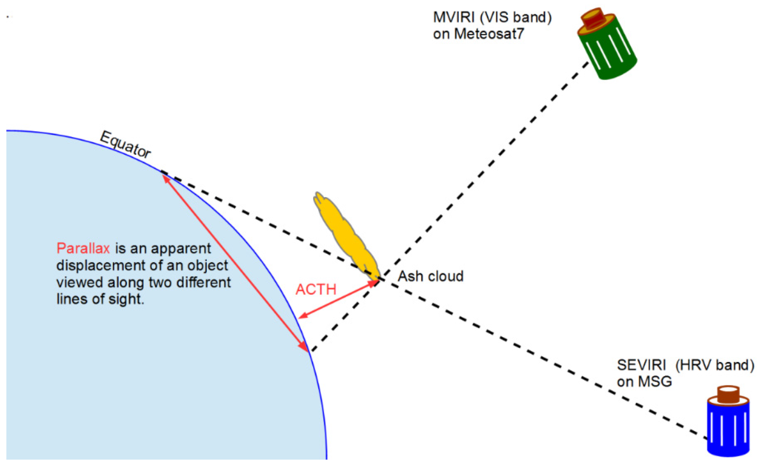
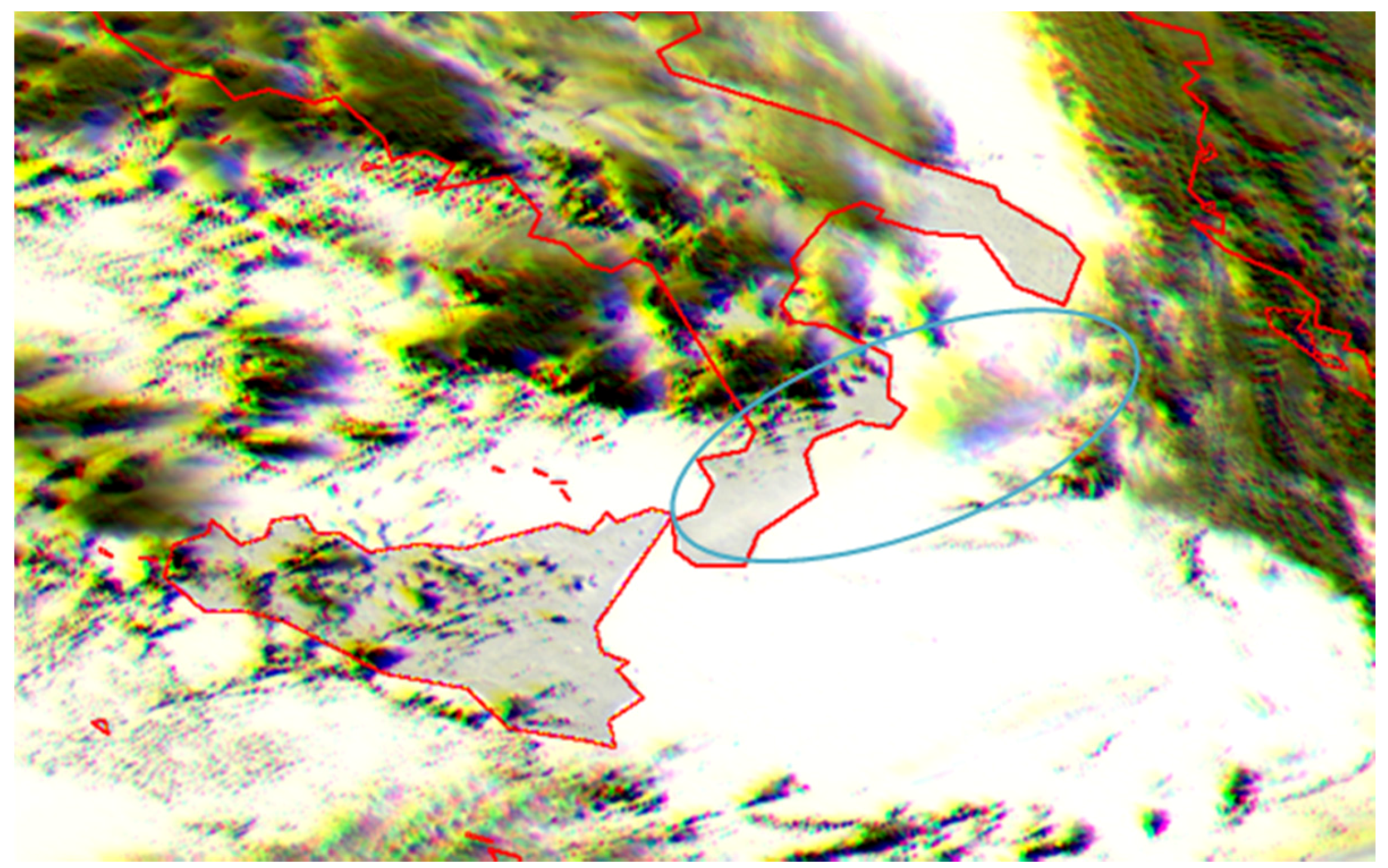
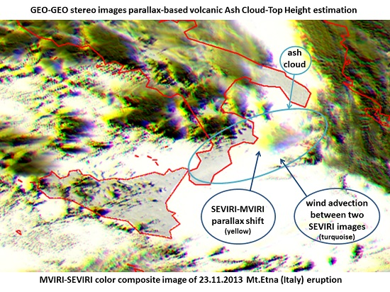
The proposed ACTH estimate is based on the apparent ash cloud displacement due to parallax, using data collected at nearly the same time by two multispectral radiometers on board different geostationary satellites. The parallax can be measured as the distance between the apparent positions of the same cloud observed from two different observation points, and it depends on the height of the cloud (see Figure 1). Since the known position of the satellites and the georeferenced images define the viewing geometry, the ACTH can easily be estimated in three steps. The MVIRI data is first projected onto the SEVIRI spatial grid. Then the images are co-registered in an automatic matching procedure. Finally, the lines of sight connecting each observed point from the two satellites are generated and their intersections are used to estimate the ACTH.

3.1. Projection of MVIRI Data onto the SEVIRI Grid

To detect parallax, the images retrieved from different satellites first have to be referenced within the same image coordinate system. This means that all data must have the same georeference, i.e., the same map projection, geodetic datum, and raster resolution. Once this is achieved, it can be observed that all objects with elevation zero (coastlines) are aligned in all images. If an object is elevated, then its position in the image coordinate system depends on its height and on the position of the satellite. All satellite data are projected in a general near-side perspective projection, which is not a standard map projection. Projections of geostationary satellites differ basically only in sub-satellite longitude. The image coordinate system also depends on the size of the image and the spatial resolution of the instrument. These data are retrieved from EUMETSAT metadata delivered as level 1.5 data. Using bilinear interpolation, the MVIRI data is reprojected from its native projection to the SEVIRI projection grid. The SEVIRI grid was chosen for reference because it is centred over the area of interest (Europe) and the SEVIRI repetition cycle is used to estimate the influence of wind.

3.2. Automatic Image Matching

The image matching identifies point pairs between two satellite images. If the images are not acquired by the same instrument, as in this case, results might be of poor quality because of differences in spatial resolution, viewing geometry, instrument response functions, and solar illumination conditions. The results of image matching are, however, usually good enough to estimate ACTH. The method used is that described by e.g., Scambos et al. [42], and Zakšek et al. [23].

Image matching estimates image shifts between pairs of images. However, in the proposed procedure, three images are always used to account for the influence of wind: one MVIRI image, and two SEVIRI images acquired just before and after the MVIRI image was retrieved. Starting from MVIRI coordinates, image matching is conducted twice to find matching points between the MVIRI and both SEVIRI images. Since the coordinates of the matched points were not retrieved at the same time as the MVIRI was collected, the position of the cloud was estimated as it would have appeared in a SEVIRI image collected at exactly the same time as the MVIRI image, by linear interpolation. Given the position of the cloud and both the satellites, the MVIRI and SEVIRI lines of sight can be generated. From the intersection of these it is easy to compute the height.

3.3. ACTH Estimation from the Intersection of Lines of Sight

After the image matching procedure, triples of geographic coordinate pairs were also determined for each pixel. The effects of possible advection of the eruption cloud between the MVIRI and the two SEVIRI data collection times is considered for each pixel triple: the coordinates of a virtual SEVIRI pixel are interpolated from the position of both the actual SEVIRI pixels to the time of the MVIRI acquisition. The conversion from geographic coordinates into geocentric Cartesian coordinates allows the final calculation based on vector algebra. The lines connecting the virtual SEVIRI pixels with the MSG satellite position (SEVIRI lines) and the corresponding lines connecting MVIRI pixels and the Meteosat-7 satellite position can be expressed as parametric equations in the 3D space. The intersection of these line pairs is ideally given by the solution of a linear system.

In practice, the linear system is over determined, and can only be solved by a least-square technique: due to the discrete nature of the datasets the MVIRI and SEVIRI lines never intersect and the solution is not a single point real intersection, but instead is given by the two points at a minimum distance between the lines. The position of one of these two points (or their average) represents the ACTH estimation result. High ACTH estimation accuracy is achieved with this procedure when the distance between the MVIRI and SEVIRI lines is small. For further details see [23].

3.4. ACTH Estimation Error

A description is now provided of the analytical solution of ACTH estimation accuracy from observations collected by two geostationary satellites.

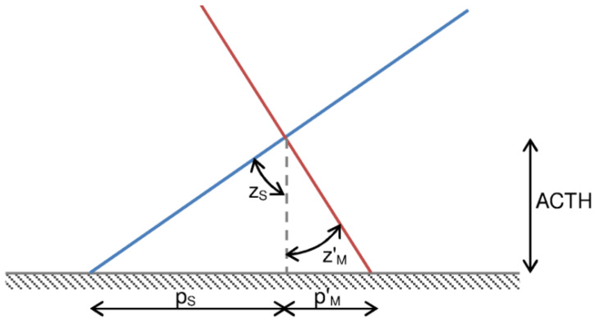
Considering the spatial resolution that meteorological satellites offer today and the height of volcanic clouds, the surface of the Earth is assumed to be flat and not curved.

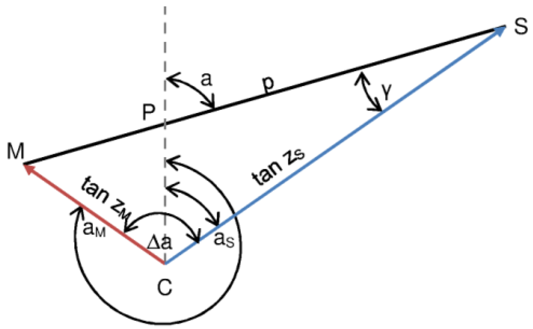
Given the zenith angle of a satellite (see Figure 2), the relationship between parallax and ACTH can be given as:

$$\tan z=\frac{p}{ACTH}$$

Parallax p can be observed only if a point is observed from at least two different positions. The parallax can, thus, be defined as the sum of two parallaxes projected to the same vertical plane:

$$p=p_S+{p^{\prime }}_M=ACTH\cdot \left(\tan z_S-\cos \Delta a\cdot \tan z_M\right)$$

In the first part of the equation above, the sign between both terms is plus, and in the second part it is minus. This is a consequence of the projection of the second parallax to the vertical plane defined by the first parallax. The projection is achieved using the cosine of the difference Δa between azimuths pointing in the directions of both parallaxes. This equation can thus also be used to estimate ACTH:

$$ACTH=\frac{p}{\tan z_S-\cos \Delta a\cdot \tan z_M}$$

(1)

To estimate the analytical accuracy of ACTH, it can be assumed that the automatic image matching provides results with errors of no more than a half a pixel. Therefore, for each pixel in the SEVIRI grid it can be estimated under which zenith and azimuth angles the pixel was observed from the SEVIRI and MVIRI positions. Zenith angle is computed from the scalar product between the vector normal to the surface and the vector to the satellite (both unit vectors). Azimuth estimation is even easier. Since the nominal latitude of geostationary satellites is zero, the azimuth a toward the satellites can be computed from:

$$\tan a=\frac{\sin \left(\lambda -{\lambda }_0\right)}{(1-e^2)\cdot \tan \phi }$$

(2)

where λ is the pixel longitude, λ₀ is the longitude of the geostationary satellite, e is the first eccentricity of the WGS84 ellipsoid, and φ the pixel latitude. Once the azimuth and zenith angles to both satellites are known for each pixel seen from both satellites, the ACTH can be estimated for a parallax that measures one single pixel. This value provides the following information: (a) an estimate of the minimum ACTH that can be reliably estimated; and (b) half this value equals the accuracy of the ACTH estimate, if the image matching provides results with a maximum error of half a pixel.

To evaluate the error on the ACTH estimate it is first necessary to compute the azimuth of the parallax, because it influences the parallax value, the parallax is greater if it is diagonal rather than columnar or linear in direction.

The triangle CSM in Figure 3 is defined by the projection of the cloud true position (point C) to the horizontal plane at sea level, the end point of the parallax from SEVIRI (point S), and the end point of the parallax from MVIRI (point M). Point P is defined by the intersection of a line running North and the parallax (p; line SM). The azimuth of the parallax a can be estimated, once all the angles in the triangle CSP or CPM are known. To estimate angle γ in the triangle CSP, first the parallax p needs to be estimated using the law of cosines (angle MCS is known from the difference of azimuths a_S and a_M, side MC corresponds to tan z_M, and side CS to tan z_S.

$$p^2={\tan }^2{z}_S+{\tan }^2{z}_M+2\cdot \tan z_S\cdot \tan z_M\cdot \cos \Delta a$$

(3)

The law of sines is then used to compute γ:

$$\sin \gamma =\frac{\sin \Delta a}{p}\cdot \tan z_M$$

(4)

Finally, azimuth a can be estimated showing the direction of the observed parallax:

$$a=a_S+\gamma$$

(5)

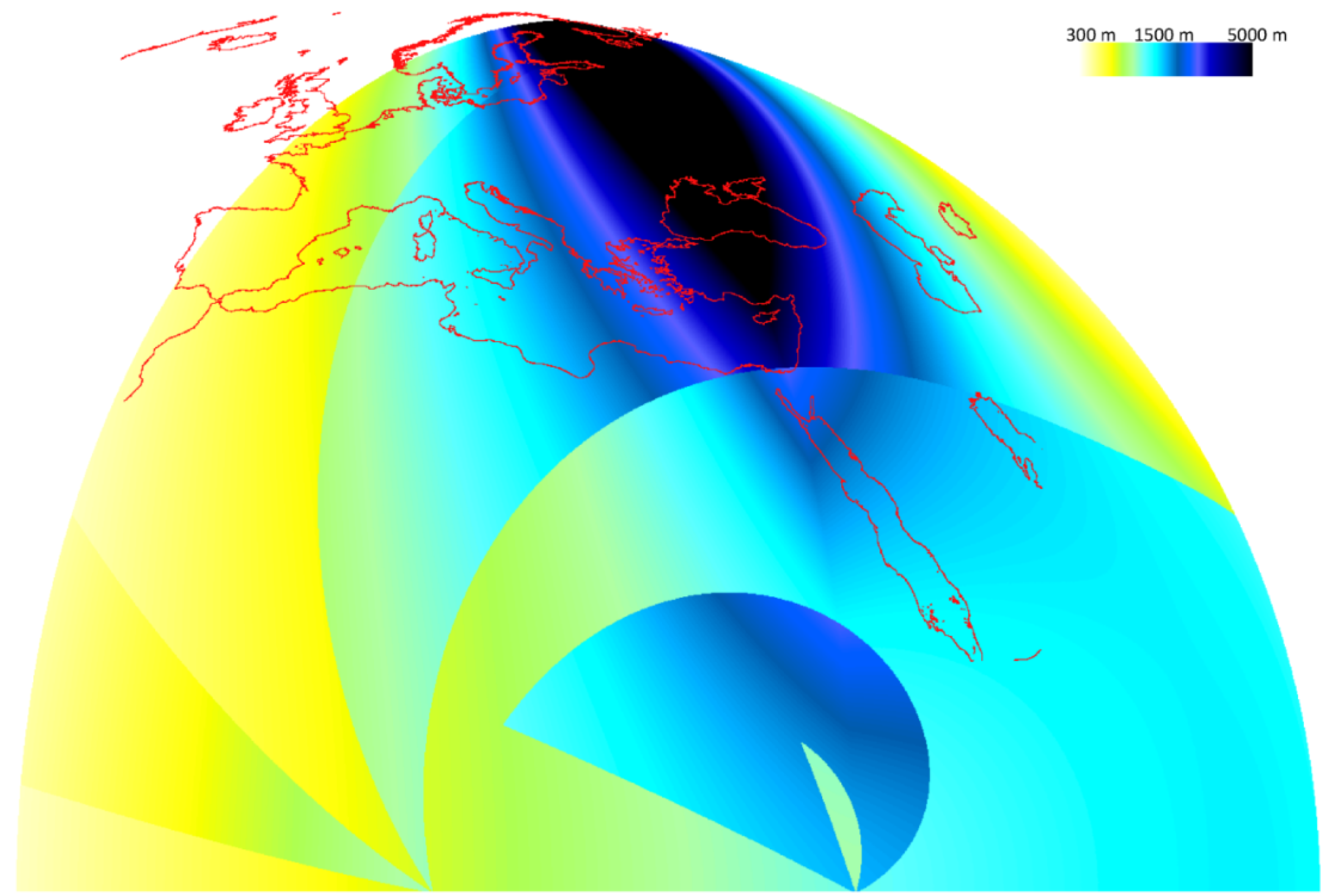
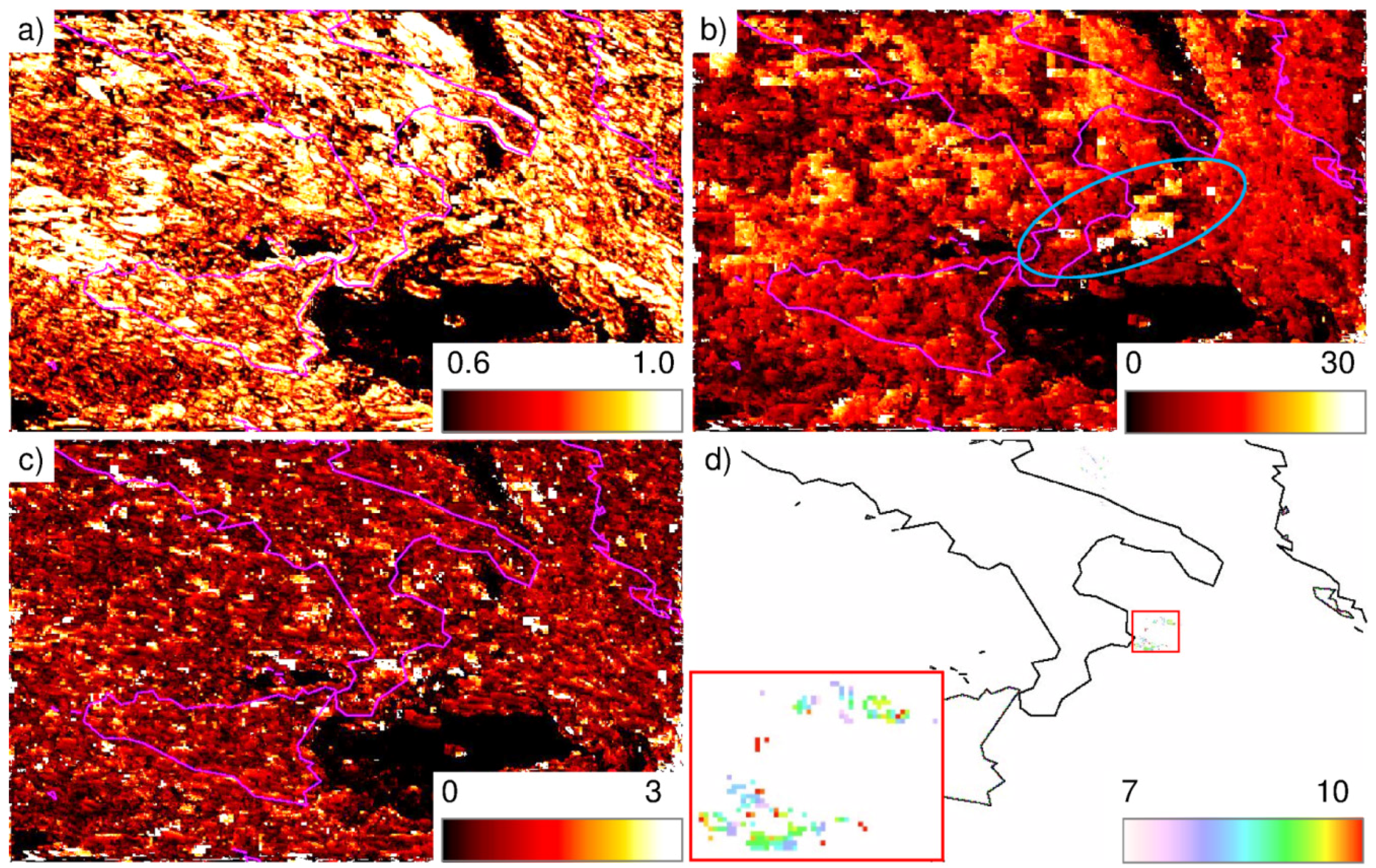
After the parallax azimuth has been estimated, it is possible to determine which neighbouring pixel is the closest in this direction. Given the distance between neighbouring pixels in this direction, Equation (1) can be used to estimate the minimal detectable ACTH. Considering the error of one single pixel, the number of possible azimuths of the parallax can be reduced to eight directions (eight neighbor pixels). Thus, one can expect discontinuities in those areas, where the azimuth of the parallax changes from one to another of the eight values. The results for the northern hemisphere of the combination of SEVIRI and MVIRI satellites are shown in Figure 4. The results are given in the grid of the SEVIRI HRV channel situated on 9.5° E. The area presented shows only the pixels for which both instruments have a zenith angle of less than 80°.

However, it is worth noting that this estimation assumed that the spatial resolution of both instruments is almost the same. Over Europe the MVIRI instrument has a significantly lower spatial resolution than SEVIRI. This has a large influence on the automatic image matching, making it difficult to properly match all the SEVIRI and MVIRI pixels.

In addition, the halves of values in Figure 1 can be interpreted as an estimate of accuracy, considering that the image matching provides an accuracy of half a pixel. Again, this is not a totally realistic estimate, since the spatial resolution of MVIRI over Europe is ~5000 m. It is therefore necessary to check all the internal measurements of accuracy first: the suggested values are realistic if correlation between SEVIRI and MVIRI is high (>0.9) for all image pyramids (see [23,43] for details) and if the estimated distance between both lines of sight is not greater than half a SEVIRI pixel.

Note that in the case of a higher cloud, the parallax would be larger than a single pixel (which is assumed in Figure 4), with the result that the discontinues in Figure 4 would be softened in the accuracy image, because the parallax would not be limited to only eight different azimuths.

4. Results

4.1. Etna 23.11.2013 Case Study

On 23 November 2013, starting at 8:00 UTC, the Strombolian activity [44,45] of the new South East Crater (NSEC) of Mt. Etna, which had started the previous day, intensified and around 9:30 UTC evolved into a lava fountain [46,47]. The emission of ash and the eruptive column height increased quickly with lava emissions reaching maximum height around 10:10 UTC. At 10:15 UTC the height of the jets dropped dramatically and at 10:20 UTC activity returned to Strombolian explosions visible until 10:55 UTC. The good weather conditions allowed acquisition of the entire eruptive event by the SEVIRI and MVIRI sensors, and these image sequences form the basis for this study.

4.2. ACTH Results

The images used to estimate the ACTH of the volcanic cloud emitted during the 23 November 2013 Mt Etna eruption are the VIS channel of the MVIRI sensor aboard the MFG (IODC) platform at longitude 57.5° E, and the HRV channel of the SEVIRI sensor in RSS mode platform on the MSG-2 backup satellite located at 9.5° E (see Section 2). The RSS mode offers the minimum difference between the image acquisition times of the two sensors (max 2.5 min), and so minimizes errors due to wind advection by applying the correction described in Section 3.2. Figure 5 shows two sample images extracted from the sequences captured by the two sensors around 11:49 UTC, with the volcanic clouds marked in blue ellipses. Note that the spatial resolution of MVIRI is significantly lower than the resolution of SEVIRI for the Mediterranean area. This is a consequence firstly of lower resolution of MVIRI at nadir and secondly of the viewing geometry—MVIRI observes Europe quite close to the hemisphere’s horizon (seen in the upper left corner of Figure 5b). Thus, the island of Sicily looks significantly smaller in the MVIRI data (spatial resolution ~5 km for Sicily) than in SEVIRI data (spatial resolution ~1 km for Sicily). Consequently, it is more difficult to see the position of the ash cloud in a single MVIRI image, while it is much easier to observe it in the SEVIRI data of Figure 5a. The volcanic cloud can easily be observed with both instruments in the animation of the complete sequences of images of the eruption provided in the supplementary data.

Once a volcanic cloud has been correctly identified, it is very important to check the co-registration of the image pairs, since the final ACTH accuracy is highly dependent on the quality of the image matching (see Section 3). A useful visual tool for a quick quality control of the results is shown in Figure 6. Here, the MVIRI image and the two SEVIRI images acquired immediately before and after the MVIRI acquisition at 11:49 UTC have been superimposed into an RGB image, with first SEVIRI as the red component, second SEVIRI as the green component, and MVIRI as the blue component. To make the image more appealing, the colours were inverted—in the original images the clouds appear bright while the sea is dark. The result is a color composite image that highlights the parallax between SEVIRI and MVIRI in yellow. The thicker the yellow belt northeast of the cloud, the greater the parallax, and the greater the cloud’s height. The turquoise colour indicates areas influenced by cloud displacement during the 5 min that elapsed between the two subsequent SEVIRI images: the thicker the turquoise belt, the faster the movement of the clouds. Everything appearing white or grey has a low elevation.

In this representation, if the images are not well co-registered these colour belts are immediately observed along the coastlines.

As already stated in Section 2, the choice to use visible channels enables estimation of the ACTH with the maximum accuracy achievable using the current operational geostationary instruments and, thus, better demonstrating the potential of the proposed height estimation scheme. Another reason is that ash cloud detection algorithms are based on channels in the thermal infrared range. The simplest effective ash cloud detection is obtained by evaluating the brightness temperature difference (BTD) defined for two channels centred at around 11 and 12 μm [48,49]. Since MVIRI has only one channel in the TIR range, the BTD cannot be evaluated, and meteorological and volcanic ash clouds cannot be discriminated based on MVIRI data. In the HRV SEVIRI image of Figure 5, a dark plume can be seen over the southern tip of the Calabria peninsula (inside the green ellipse) extending into a brighter cloud (marked by the yellow ellipse) over the western part of the Ionian Sea. The dark part of the plume is recognized as ash using BTD and the bright part as a meteorological cloud. Given that both are of volcanic origin, the focus here is only on the bright part of the cloud (which is probably composed of a mixture of ash and ice crystals or water droplets [50]), because the dark part of the plume is too transparent to be clearly detected in the visible bands. This brighter, highly-reflective cloud can be observed with both instruments and is used here to apply the ACTH estimation method.

Figure 7 shows the final results for the same scene presented in Figure 5. Figure 7a shows the correlation between the MVIRI and SEVIRI data prior to the MVIRI observation. It is low for most pixels because of the low level of detail in MVIRI: the spatial resolution of MVIRI is very coarse compared to SEVIRI. Over the bright volcanic cloud, the correlation is only high (>0.95) on the northern and southern edge of the cloud (in white), otherwise it is below 0.8. Figure 7b presents the computed parallax: the bright areas in the blue ellipse represent 30 km, and orange to yellow areas about 20 km parallax. It appears quite “blocky” because there was good correlation over a coarser pyramid level, but the finer pyramids are not highly enough correlated and so the estimated shift in column and line direction is preserved from the lower pyramid.

The distance between the intersecting lines is related to the accuracy of the ACTH estimate (Figure 7c). The lines of sight never intersect because the data used have finite resolution. Thus, the closest points on both lines are determined and the distance between these points is a measure of the uncertainty of the results, which should be as small as possible. Here, only the darkest pixels are used for height estimation since they have distances between the points of less than 600 m (half a SEVIRI HRV pixel in the case study area). Several pixels were discarded because they did not correspond to the volcanic cloud, because the distance between the intersecting lines was too large (>600 m), or because the retrieved height was too low (the cloud height was assumed to be > 3 km, given the meteorological conditions and Etna’s altitude of 3300 m.a.s.l.). Moreover, the final ACTH was estimated only for the pixels selected as definitely belonging to the volcanic cloud by visual inspection of the images. The pixels in red in Figure 7d are higher than 10 km, reaching almost 11 km, the purple are lower than 7 km, and the majority of them have values of ~8–9 km (in turquoise and green and yellow).

Following the same procedure described for the two sample images of Figure 5, the ACTH distribution was analyzed for six image pairs between 10:49 and 13:19 UTC. The data collected before this time also contain a clear volcanic plume, but the image matching procedure did not provide reliable results because of the marked heterogeneity of the surface beneath the cloud, which was located over or near land. The results are summarized in the histograms shown in Figure 8, representing the evolution of the ACTH estimated with the parallax method. Not even the initial situation at 10:49 is optimal, but it can still be seen that 50% of the volcanic cloud has its ACTH in the range between 8 and 8.5 km. In the following situation it can be observed that 50% of the volcanic cloud has its ACTH in the range between 8 and 9.5 km. The highest pixels are as high as 11 km. The distribution appears to shift towards lower ACTHs with time.

4.3. Validation

The results obtained for the eruption are also in close agreement with those independently estimated with integrated measurements provided by the Mt. Etna video surveillance camera, by the radar of the Fontanarossa airport of Catania (Sicily), by applying a simpler scheme for parallax height estimation obtained from a comparison of MODIS and SEVIRI satellite data, with the IASI retrieval based on optimal estimation, and with the results obtained from the HYSPLIT model. All these estimates of the ash cloud height released during the Mt. Etna eruption event on 23 November 2013 are in close agreement with the results obtained herein and are thoroughly presented and discussed in a separate article by Corradini et al. [50] in this special issue.

The results of ACTH can be compared with those obtained from radiosonde profiles of temperature and wind speed acquired on 23 November 2013 at 12:00 UTC by the WMO meteorological station of Trapani (Sicily, Italy). From these profiles and the SEVIRI images, two different independent estimates of the cloud height can be easily obtained. Firstly, by estimating the brightness temperature of the cloud and comparing it with the temperature radiosonde vertical profile. This method, also known as darkest pixel method [51], was applied on the six SEVIRI images closest to the MVIRI images from 10:49 to 13:19 UTC with retrieved temperatures between −43.7 and −52.0 °C. The resulting cloud heights range from about less than 9 to 11 km (see Figure 9a). Secondly, by evaluating a wind speed of 38.7 m·s⁻¹ from the displacement of similar structures measured on two SEVIRI images divided by the elapsed time between the two acquisitions. This wind speed was then compared to the radiosonde wind speed vertical profile (see Figure 9b). This method is very simple, but prone to error if the reference structures identified in the cloud are not clearly maintained in the two images. In this case it can be assumed as indicative of a good agreement with an acceptable accuracy not better that 2 m·s⁻¹.

5. Discussion

There follows a discussion of the most relevant characteristics of the proposed method. Compared to other methods, the one under discussion requires two satellites that can observe the same area nearly simultaneously. Its main drawback is that the accuracy of the results is dependent on the positional accuracy of the input images. It is not particularly important for the absolute geolocation to be accurate, but the co-registration between the images from both satellites must fit perfectly. For this reason it makes sense to check the co-registration accuracy during pre-processing when all datasets are transposed to the same coordinate system. This can be done automatically by adjusting the co-registration along coastlines.

The automatic image matching, which takes the most of the processing time, requires texture or structure in clouds. Without any texture, matching points in different images cannot be found, possibly leaving only some points on the edges of the cloud where ACTH can be estimated. Normally this is not an issue, as volcanoes usually erupt in pulses which are visible in volcanic clouds. Texture might be a problem only if the spatial resolution of the input data is very fine (finer than 50 m) or too coarse (coarser than 5000 m). Considering SEVIRI, volcanic and meteorological clouds usually have enough structure in the HRV channel. Conversely, MVIRI is more problematic. It does provide significant texture close to its nadir, but in the present case study area, the spatial resolution is almost too coarse to provide enough texture. In addition, MVIRI acquires only 8-bit data in the VIS channel, meaning that fine texture details cannot be resolved as well as in SEVIRI (10-bit).

Another significant limitation is cloud transparency. According to Corradini et al. [50], the 550 nm AOD of the ash cloud was below 0.5. The ash part of Etna’s cloud could not be accurately identified with SEVIRI’s HRV channel, nor with MVIRI’s VIS channel. However, even if the cloud can be observed with a satellite instrument, it might still be so transparent that the automatic image matching is distracted by the details of the underlying surface visible through the cloud. This is not a problem over homogeneous surfaces like ocean or desert, but it can be over areas with diversity in land cover.

One of the main advantages of cloud photogrammetry is its independence from ancillary datasets or assumptions on the atmosphere state at the moment of the data acquisition. It is not important if the cloud is below the tropopause or above it. Emissivity of the cloud is irrelevant. There is no need for auxiliary data like temperature or humidity profiles.

Moreover, the proposed method is fast. The case study area of 720 by 450 pixels was processed on a notebook with a four-core Intel i7 processor in 30 s. It is also worth noting that the ACTH code was written in IDL, which is a high-level language useful for algorithm development, but probably not the fastest solution for coding real-time applications. In the present example only 10% of the processing time was used for pre-processing the MVIRI data. A similar pre-processing took much longer for the MODIS data [23] because of its finer spatial resolution, but still only about 60 s were required to process a whole 250 m MODIS image.

The most important characteristic of the method is its accuracy, discussed in Section 3. This is a factor of about three times higher than the expected accuracy of operational height estimates based on CO₂ absorption [22], and less than a factor of four times lower than that achievable with space-based LiDARs [18]. For the case study area the analytical estimate of the ACTH accuracy is 700 m.

As mentioned in Section 2, in this study only the visible channels of both instruments were used. This choice allowed exploitation of the much better spatial resolution of these channels compared to those in the thermal infrared range (at nadir, 2.5 and 1 km in the visible, vs. 5 and 3 km in the TIR for MVIRI and SEVIRI respectively), thus obtaining the most accurate ACTH estimation results achievable with these two geostationary instruments. Conversely, this choice limits the use of the method to daylight hours. Another drawback is the difficulty of obtaining a reliable detection of a volcanic ash cloud from a single image in the visible range. Fundamental for this purpose are both the fixed observation point and the high repetition cycle of geostationary sensors, which allow acquisition of a complete sequence of images of an eruption. It is, thus, possible to follow the evolution of a cloud following its emission from the volcano vent. Tracking its trajectory in this way provides proof of the volcanic origin of the cloud even at great distances from the source.

Having detected and tracked a volcanic cloud, the next step is to verify its ash composition. To achieve this (although only at reduced resolution), it is possible to use ash inverted absorption in the SEVIRI bands centred at 10.8 and 12 μm. This can be detected using the brightness temperature difference (BTD) [48] which, under certain conditions [49], allows differentiation between meteorological and volcanic clouds. As previously mentioned in Section 4, this verification is not possible with MVIRI since it only has one thermal infrared band centred at 11.5 μm.

It should be noted that the Mt. Etna eruption discussed in this article was chosen to describe the parallax method applied to geostationary satellites using available data because it is a small eruption, difficulty to detect and characterize, and suitable to reveal the problems that this approach can have. The method works well with a huge eruption releasing an extended ash cloud over the ocean, as already demonstrated by Zakšek et al. [23] for the 2010 Eyjafjallajökull eruption, although with a different sensor pair on GEO and LEO platforms with higher spatial resolution. Furthermore, the ACTH estimation presented here refers to a cloud for which a visual inspection of both image sequences identifies as being of clear volcanic origin. Conversely, the positive BTD that can be found on the SEVIRI images of the same part of the volcanic cloud used for the ACTH estimate, does not detect it as composed of volcanic ash, but rather of ice or water droplets [50]. Nevertheless, this case study is very useful to demonstrate the potential of the proposed method which, in principle, can be used to estimate the ACTH of any type of cloud using GEO multispectral imagers, regardless of whether they are volcanic ash or SO₂ clouds derived from a detection and retrieval procedure, or meteorological clouds directly identified in the satellite datasets.

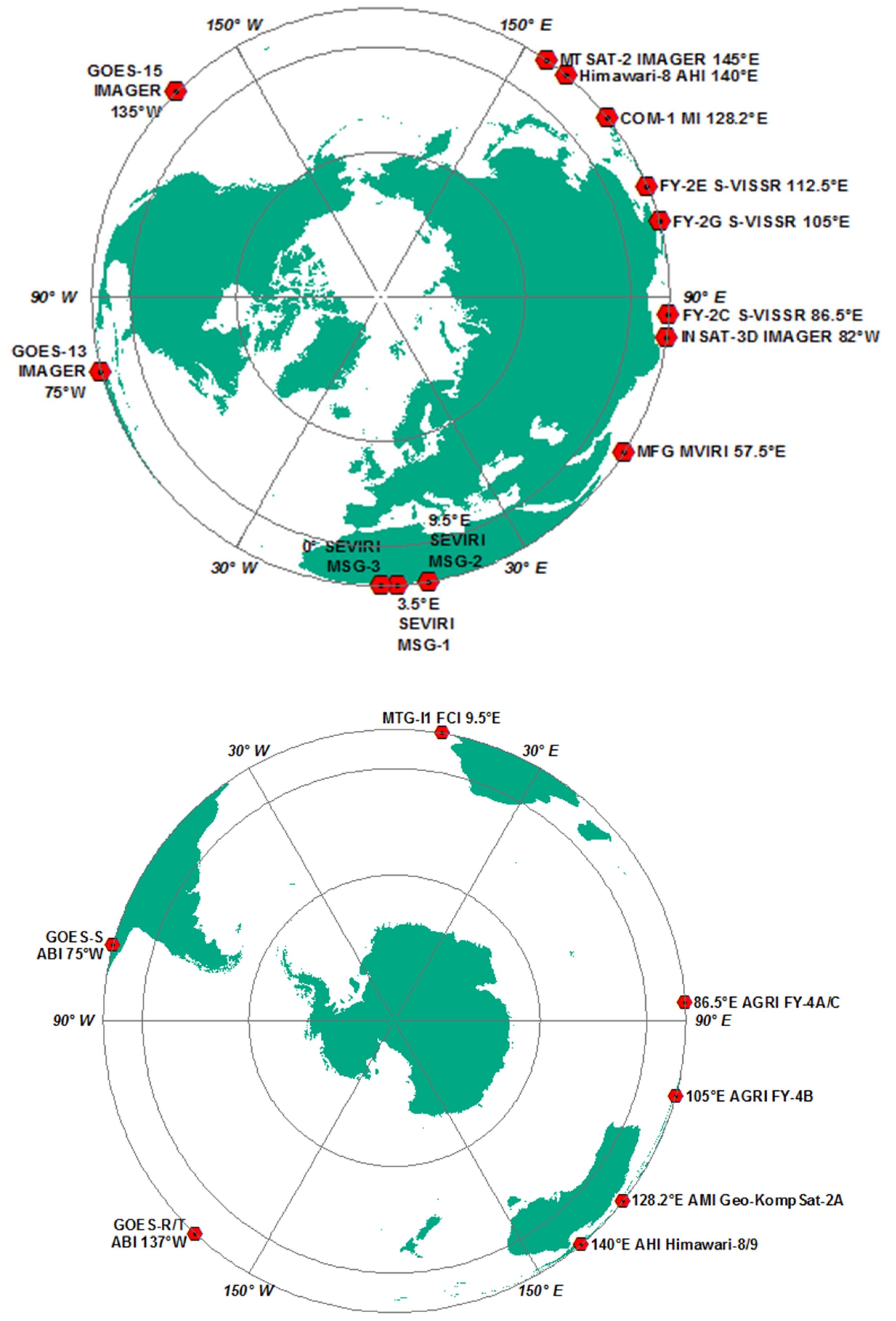
Another point is that although volcanic ash detection and retrieval is feasible with several currently operational sensors (i.e., IMAGER on GOES-13 and -15, and MTSAT-2), their spatial resolution is still too coarse to fully exploit the proposed ACTH method. The multi-purpose VIS/IR imagery capability from GEO platforms, as defined by the World Meteorological Organization, is already partly implemented with a number of medium-resolution multi-channel radiometers operating in the VIS and IR range in geostationary orbit. The reference observing strategy consists of six evenly spaced 60° wide sectors along the equator with at least one SEVIRI-class instrument per sector and a backup instrument as similar as possible nearby.

However, in the near future the situation will improve significantly. The new generation multispectral sensors—i.e., Flexible Combined Imager on MTG-I, Advanced Baseline Imager, Advanced Himawari Imager, Advanced Geostationary Radiation Imager, Electro-GOMS Imager for Electro M (MSU-GSM)—onboard geostationary platforms will have many more bands and a thermal infrared spatial resolution comparable to that currently achieved by the SEVIRI HRV visible channel [52]. After the year 2020 it is expected that all sectors will be covered with redundancy by third generation imagers, except sector 180° ± 30°, which lacks backup. Nevertheless, even this latter sector will be partially covered by instruments on board the Himawari and GOES-W platforms (see Figure 10).

The GEO VIS/IR imagery will benefit from ever-improving sensor spatial and spectral resolutions, acquisition repetition cycles, and differences in angle of view between the sensors. All these improvements will enable full advantage to be taken of the proposed method both day and night for effective monitoring of volcanic clouds on a global scale.

6. Conclusions

A volcanic ash cloud-top height estimation method was proposed, based on the apparent shift due to parallax of images collected by the multispectral imagers MVIRI and SEVIRI on board two different geostationary satellites. Previously introduced by Zakšek et al. [23] for polar and geostationary image pairs, the method was improved here with detailed discussion of its accuracy, and applied to the case study of the Mt. Etna (Sicily, Italy) eruption that occurred on 23 November 2013. The estimated ACTH for the ash cloud released during this Mt. Etna eruption was presented and discussed. Close agreement was demonstrated with the radiosounding profiles acquired by the Trapani WMO meteorological station. Further sources for the validation of the estimated ACTH can be found in a separate article [50] in this special issue. These include independent ash cloud height assessment based on space-based (SEVIRI, MODIS, IASI) measurements, ground-based (radar and surveillance video camera deployed close to Mt. Etna), and ash cloud trajectories obtained with the HYSPLIT model.

The methodology is straightforward, fast, and can valuably complement other techniques currently used for ACTH estimation. The novel application of ACTH estimates to datasets collected by instruments aboard geostationary platforms opens the way to fully exploit the potential of this methodology. It could also be immediately applied to other combinations of geostationary sensors, for instance the SEVIRI-GOES pair, but is still limited by its dependence on visible data, which provides the finest spatial resolution. However, the forthcoming launch of the next generation of meteorological multispectral imagers into geostationary orbits, offering finer spatial resolutions than current systems including infrared channels with global coverage, will allow application of the proposed method for continuous monitoring of ash clouds. This will not only increase the accuracy of results, but will also increase the applicability and effectiveness of the method. The proposed method will therefore also be applicable to meteorological clouds, other natural aerosol clouds, and even to clouds resulting from industrial accidents.

References

1. Heinold, B.; Tegen, I.; Wolke, R.; Ansmann, A.; Mattis, I.; Minikin, A.; Schumann, U.; Weinzierl, B. Simulations of the 2010 Eyjafjallajökull volcanic ash dispersal over Europe using COSMO–MUSCAT. Atmos. Environ. 2012, 48, 195–204. [Google Scholar] [CrossRef]
2. Wen, S.; Rose, W.I. Retrieval of sizes and total masses of particles in volcanic clouds using AVHRR bands 4 and 5. J. Geophys. Res. Atmos. 1994, 99, 5421–5431. [Google Scholar] [CrossRef]
3. Prata, A.J.; Grant, I.F. Retrieval of microphysical and morphological properties of volcanic ash plumes from satellite data: Application to Mt Ruapehu, New Zealand. Q. J. Royal Meteorol. Soc. 2001, 127, 2153–2179. [Google Scholar] [CrossRef]
4. Corradini, S.; Merucci, L.; Prata, A.J. Retrieval of SO2 from thermal infrared satellite measurements: Correction procedures for the effects of volcanic ash. Atmos. Meas. Tech. 2009, 2, 177–191. [Google Scholar] [CrossRef]
5. Mastin, L.G.; Guffanti, M.; Servranckx, R.; Webley, P.; Barsotti, S.; Dean, K.; Durant, A.; Ewert, J.W.; Neri, A.; Rose, W.I.; et al. A multidisciplinary effort to assign realistic source parameters to models of volcanic ash-cloud transport and dispersion during eruptions. J. Volcanol. Geotherm. Res. 2009, 186, 10–21. [Google Scholar] [CrossRef]
6. Stohl, A.; Prata, A.J.; Eckhardt, S.; Clarisse, L.; Durant, A.; Henne, S.; Kristiansen, N.I.; Minikin, A.; Schumann, U.; Seibert, P.; et al. Determination of time- and height-resolved volcanic ash emissions and their use for quantitative ash dispersion modeling: The 2010 Eyjafjallajökull eruption. Atmos. Chem. Phys. 2011, 11, 4333–4351. [Google Scholar] [CrossRef] [Green Version]
7. Rose, W.I.; Kostinski, A.B.; Kelley, L. Real-time C-band radar observations of 1992 eruption clouds from Crater Peak, Mount Spurr volcano, Alaska. US Geol. Surv. Bull. 1995, 2139, 19–26. [Google Scholar]
8. Lacasse, C.; Karlsdóttir, S.; Larsen, G.; Soosalu, H.; Rose, W.I.; Ernst, G.G.J. Weather radar observations of the Hekla 2000 eruption cloud, Iceland. Bull. Volcanol. 2003, 66, 457–473. [Google Scholar] [CrossRef]
9. Marzano, F.S.; Lamantea, M.; Montopoli, M.; Di Fabio, S.; Picciotti, E. The Eyjafjöll explosive volcanic eruption from a microwave weather radar perspective. Atmos. Chem. Phys. 2011, 11, 9503–9518. [Google Scholar] [CrossRef] [Green Version]
10. Scollo, S.; Prestifilippo, M.; Pecora, E.; Corradini, S.; Merucci, L.; Spata, G.; Coltelli, M. Eruption column height estimation of the 2011–2013 Etna lava fountains. Ann. Geophys. 2014, 57, S0214. [Google Scholar]
11. Scollo, S.; Boselli, A.; Coltelli, M.; Leto, G.; Pisani, G.; Spinelli, N.; Wang, X. Monitoring Etna volcanic plumes using a scanning LiDAR. Bull. Volcanol. 2012, 74, 2383–2395. [Google Scholar] [CrossRef]
12. Wang, X.; Boselli, A.; D’Avino, L.; Pisani, G.; Spinelli, N.; Amodeo, A.; Chaikovsky, A.; Wiegner, M.; Nickovic, S.; Papayannis, A.; et al. Volcanic dust characterization by EARLINET during Etna’s eruptions in 2001–2002. Atmos. Environ. 2008, 42, 893–905. [Google Scholar] [CrossRef]
13. Emeis, S.; Forkel, R.; Junkermann, W.; Schäfer, K.; Flentje, H.; Gilge, S.; Fricke, W.; Wiegner, M.; Freudenthaler, V.; Groβ, S.; et al. Measurement and simulation of the 16/17 April 2010 Eyjafjallajökull volcanic ash layer dispersion in the northern Alpine region. Atmos. Chem. Phys. 2011, 11, 2689–2701. [Google Scholar] [CrossRef]
14. Gasteiger, J.; Groß, S.; Freudenthaler, V.; Wiegner, M. Volcanic ash from Iceland over Munich: Mass concentration retrieved from ground-based remote sensing measurements. Atmos. Chem. Phys. 2011, 11, 2209–2223. [Google Scholar] [CrossRef]
15. Hervo, M.; Quennehen, B.; Kristiansen, N.I.; Boulon, J.; Stohl, A.; Fréville, P.; Pichon, J.-M.; Picard, D.; Labazuy, P.; Gouhier, M.; et al. Physical and optical properties of 2010 Eyjafjallajökull volcanic eruption aerosol: Ground-based, Lidar and airborne measurements in France. Atmos. Chem. Phys. 2012, 12, 1721–1736. [Google Scholar] [CrossRef] [Green Version]
16. Merucci, L.; Burton, M.; Corradini, S.; Salerno, G.G. Reconstruction of SO2 flux emission chronology from space-based measurements. J. Volcanol. Geotherm. Res. 2011, 206, 80–87. [Google Scholar] [CrossRef]
17. Genkova, I.; Seiz, G.; Zuidema, P.; Zhao, G.; Di Girolamo, L. Cloud top height comparisons from ASTER, MISR, and MODIS for trade wind cumuli. Remote Sens. Environ. 2007, 107, 211–222. [Google Scholar] [CrossRef]
18. Winker, D.M.; Liu, Z.; Omar, A.; Tackett, J.; Fairlie, D. CALIOP observations of the transport of ash from the Eyjafjallajökull volcano in April 2010. J. Geophys. Res. 2012, 117, D00U15. [Google Scholar] [CrossRef]
19. Winker, D.M.; Pelon, J.; Coakley, J.A.J.; Ackerman, S.A.; Charlson, R.J.; Colarco, P.R.; Flamant, P.; Fu, Q.; Hoff, R.M.; Kittaka, C.; et al. The CALIPSO Mission: A Global 3D View of Aerosols and Clouds. Bull. Am. Meteorol. Soc. 2010, 91, 1211. [Google Scholar] [CrossRef]
20. Wiegner, M.; Madonna, F.; Binietoglou, I.; Forkel, R.; Gasteiger, J.; Geiß, A.; Pappalardo, G.; Schäfer, K.; Thomas, W. What is the benefit of ceilometers for aerosol remote sensing? An answer from EARLINET. Atmos. Meas. Tech. 2014, 7, 1979–1997. [Google Scholar] [CrossRef]
21. Frey, R.A.; Baum, B.A.; Menzel, W.P.; Ackerman, S.A.; Moeller, C.C.; Spinhirne, J.D. A comparison of cloud top heights computed from airborne lidar and MAS radiance data using CO2 slicing. J. Geophys. Res. 1999, 104, 24547–24555. [Google Scholar] [CrossRef]
22. Holz, R.E.; Ackerman, S.A.; Nagle, F.W.; Frey, R.; Dutcher, S.; Kuehn, R.E.; Vaughan, M.A.; Baum, B. Global Moderate Resolution Imaging Spectroradiometer (MODIS) cloud detection and height evaluation using CALIOP. J. Geophys. Res. 2008, 113, D00A19. [Google Scholar] [CrossRef]
23. Zakšek, K.; Hort, M.; Zaletelj, J.; Langmann, B. Monitoring volcanic ash cloud top height through simultaneous retrieval of optical data from polar orbiting and geostationary satellites. Atmos. Chem. Phys. 2013, 13, 2589–2606. [Google Scholar] [CrossRef]
24. Carn, S.A.; Pallister, J.S.; Lara, L.; Ewert, J.W.; Watt, S.; Prata, A.J.; Thomas, R.J.; Villarosa, G. The Unexpected Awakening of Chaitén Volcano, Chile. Eos. Trans. AGU 2009, 90, 205–206. [Google Scholar] [CrossRef]
25. Kursinski, E.R.; Hajj, G.A.; Schofield, J.T.; Linfield, R.P.; Hardy, K.R. Observing Earth’s atmosphere with radio occultation measurements using the Global Positioning System. J. Geophys. Res. 1997, 102, 23429–23465. [Google Scholar] [CrossRef]
26. Solheim, F.S.; Vivekanandan, J.; Ware, R.H.; Rocken, C. Propagation delays induced in GPS signals by dry air, water vapor, hydrometeors, and other particulates. J. Geophys. Res. 1999, 104, 9663–9670. [Google Scholar] [CrossRef]
27. Oppenheimer, C. Review article: Volcanological applications of meteorological satellites. Int. J. Remote Sens. 1998, 19, 2829–2864. [Google Scholar] [CrossRef]
28. Eckhardt, S.; Prata, A.J.; Seibert, P.; Stebel, K.; Stohl, A. Estimation of the vertical profile of sulfur dioxide injection into the atmosphere by a volcanic eruption using satellite column measurements and inverse transport modeling. Atmos. Chem. Phys. 2008, 8, 3881–3897. [Google Scholar] [CrossRef]
29. Dubuisson, P.; Frouin, R.; Dessailly, D.; Duforêt, L.; Léon, J.-F.; Voss, K.; Antoine, D. Estimating the altitude of aerosol plumes over the ocean from reflectance ratio measurements in the O2 A-band. Remote Sens. Environ. 2009, 113, 1899–1911. [Google Scholar] [CrossRef]
30. Richards, M.S. Volcanic Ash Cloud Heights Using the MODIS CO2-Slicing Algorithm. M.Sc. Thesis, University of Wisconsin, Madison, WI, USA, 6 January 2006. [Google Scholar]
31. Chang, F.-L.; Minnis, P.; Lin, B.; Khaiyer, M.M.; Palikonda, R.; Spangenberg, D.A. A modified method for inferring upper troposphere cloud top height using the GOES 12 imager 10.7 and 13.3 μm data. J. Geophys. Res. 2010, 115, D06208. [Google Scholar]
32. Glaze, L.S.; Francis, P.W.; Self, S.; Rothery, D.A. The 16 September 1986 eruption of Lascar volcano, North Chile: Satellite investigations. Bull. Volcanol. 1989, 51, 149–160. [Google Scholar] [CrossRef]
33. Hasler, A.F. Stereographic observations from geosynchronous satellites: An important new tool for the atmospheric sciences. Bull. Amer. Meteor. Soc. 1981, 62, 194–212. [Google Scholar] [CrossRef]
34. Prata, A.J.; Turner, P.J. Cloud-top height determination using ATSR data. Remote Sens. Environ. 1997, 59, 1–13. [Google Scholar] [CrossRef]
35. Scollo, S.; Kahn, R.A.; Nelson, D.L.; Coltelli, M.; Diner, D.J.; Garay, M.J.; Realmuto, V.J. MISR observations of Etna volcanic plumes. J. Geophys. Res. 2012, 117, D06210. [Google Scholar] [CrossRef]
36. Virtanen, T.H.; Kolmonen, P.; Rodríguez, E.; Sogacheva, L.; Sundström, A.-M.; de Leeuw, G. Ash plume top height estimation using AATSR. Atmos. Meas. Tech. 2014, 7, 2437–2456. [Google Scholar] [CrossRef] [Green Version]
37. Carboni, E.; Grainger, R.G.; Thomas, G.E.; Poulsen, C.A.; Siddans, R.; Smith, A.; Sayer, A.; Peters, D. Volcanic Plume Characterization Using Satellite Measurements in the Visible and Thermal Infrared; USEReST Workshop: Neaples, Italy, 2008. [Google Scholar]
38. Francis, P.N.; Cooke, M.C.; Saunders, R.W. Retrieval of physical properties of volcanic ash using Meteosat: A case study from the 2010 Eyjafjallajökull eruption. J. Geophys. Res. 2012, 117, D00U09. [Google Scholar] [CrossRef]
39. Pavolonis, M.J.; Heidinger, A.K.; Sieglaff, J. Automated retrievals of volcanic ash and dust cloud properties from upwelling infrared measurements. J. Geophys. Res. Atmos. 2013, 118, 1436–1458. [Google Scholar] [CrossRef]
40. Poulsen, C.A.; Siddans, R.; Thomas, G.E.; Sayer, A.M.; Grainger, R.G.; Campmany, E.; Dean, S.M.; Arnold, C.; Watts, P.D. Cloud retrievals from satellite data using optimal estimation: Evaluation and application to ATSR. Atmos. Meas. Tech. 2012, 5, 1889–1910. [Google Scholar] [CrossRef]
41. Stoter, A. Observations of the Karthala Eruption, Mph Report; University of Oxford: Oxford, UK, 2009. [Google Scholar]
42. Scambos, T.A.; Dutkiewicz, M.J.; Wilson, J.C.; Bindschadler, R.A. Application of image cross-correlation to the measurement of glacier velocity using satellite image data. Remote Sens. Environ. 1992, 42, 177–186. [Google Scholar] [CrossRef]
43. Adelson, E.H.; Anderson, C.H.; Bergen, J.R.; Burt, P.J.; Ogden, J.M. Pyramid methods in image processing. RCA Eng. 1984, 29, 33–41. [Google Scholar]
44. Valentine, G.A.; Gregg, T.K.P. Continental basaltic volcanoes—Processes and problems. J. Volcanol. Geotherm. Res. 2008, 177, 857–873. [Google Scholar] [CrossRef]
45. Vergniolle, S.; Ripepe, M. From Strombolian explosions to fire fountains at Etna Volcano (Italy): What do we learn from acoustic measurements? Geol. Soc. Lond. Spec. Publ. 2008, 307, 103–124. [Google Scholar] [CrossRef]
46. UFVG Rapporto UFVG del 28 Novembre 2013: L’attività Parossistica del 23 Novembre 2013 al Nuovo Cratere di SE: Dispersione del Deposito di Caduta e Caratteristiche dei Prodotti Eruttati. Available online: http://www.ct.ingv.it/it/rapporti/vulcanologia.html?view=docman (accessed on 25 February 2016).
47. Bollettino settimanale sul monitoraggio vulcanico, geochimico e sismico del vulcano Etna 26/11/2013. Available online: http://www.ct.ingv.it/it/rapporti/multidisciplinari.html?view=docman&start=210 (accessed on 25 February 2016).
48. Prata, A.J. Observations of volcanic ash clouds in the 10–12 μm window using AVHRR/2 data. Int. J. Remote Sens. 1989, 10, 751–761. [Google Scholar] [CrossRef]
49. Prata, F.; Bluth, G.; Rose, B.; Schneider, D.; Tupper, A. Comments on “Failures in detecting volcanic ash from a satellite-based technique”. Remote Sens. Environ. 2001, 78, 341–346. [Google Scholar] [CrossRef]
50. Corradini, S.; Montopoli, M.; Guerrieri, L.; Ricci, M.; Scollo, S.; Merucci, L.; Marzano, F.S.; Pugnaghi, S.; Prestifilippo, M.; Ventress, L.J.; et al. A Multi-Sensor Approach for Volcanic Ash Cloud Retrieval and Eruption Characterization: The 23 November 2013 Etna Lava Fountain. Remote Sens. 2016, 8, 58. [Google Scholar] [CrossRef]
51. Corradini, S.; Merucci, L.; Prata, A.J.; Piscini, A. Volcanic ash and SO2 in the 2008 Kasatochi eruption: Retrievals comparison from different IR satellite sensors. J. Geophys. Res. 2010, 115, D00L21. [Google Scholar]
52. WMO, OSCAR. Available online: http://www.wmo-sat.info/oscar/ (accessed on 25 February 2016).
53. WMO, OSCAR. Available online: http://www.wmo-sat.info/oscar/observingmissions/view/2 (accessed on 25 February 2016).
Figure 1. The scheme of observations as seen by an observer above the North pole; the lines of sight from two satellites cross at one point. Its coordinates are easy to determine within the Cartesian geocentric coordinates system. Conversion to geodetic coordinates gives us ACTH.
Remotesensing 08 00206 g001
Figure 2. The scheme of observations of a cloud from two directions (subscripts at the parallax p and zenith angle z correspond to S for the blue line directed to SEVIRI and M for the red line directed to MVIRI). The cloud is positioned at the intersection of the coloured lines. The scheme presents the plane defined by the normal to the WGS84 ellipsoid and the direction of the longest parallax (here the blue line). The other line is projected (the apostrophe on the symbol denotes that the parameter has been projected on the same plane by multiplying the parallax by the cosine of the angle between the red and blue lines).
Remotesensing 08 00206 g002
Figure 3. The scheme of the lines of sight (lines connecting points MC and CS) projected to the horizontal plane from two satellites (in colour) forming the corresponding parallax p (MS); both lines of sight are presented as vectors that start in the nadir point of the cloud C and end at the position observed by the satellites (M and S, for MVIRI and SEVIRI, respectively). The zenith and azimuth angles to the satellites are known for both points and the azimuth a of the parallax needs to be estimated.
Remotesensing 08 00206 g003
Figure 4. The minimum detectable cloud height considering that a parallax of exactly one pixel is observed. Note the discontinuities—the data depends on the direction of parallax—if it indicates a diagonal neighboring pixel, the results will be greater than when parallax indicates a neighboring pixel along the same line or column.
Remotesensing 08 00206 g004
Figure 5. The Etna 23.11.2013 eruption viewed in the images collected around 11:49 UTC from (a) SEVIRI (9.5° E); and (b) MVIRI (57.5° E). The cloud of volcanic origin is marked with a blue ellipse. The cloud for which ACTH is estimated is marked in yellow. The ash cloud marked in green is not visible in the MVIRI image. The complete sequence of SEVIRI and MVIRI images is provided in the supplementary material.
Remotesensing 08 00206 g005
Figure 6. Color composite image representing the comparison of the situation as seen by the two sensors at about 11:49 UTC. This figure visually highlights the parallax between MVIRI and SEVIRI in yellow, and the effects of wind between the two SEVIRI images in turquoise. The volcanic cloud is marked by a blue ellipse.
Remotesensing 08 00206 g006
Figure 7. (a) Correlation; (b) parallax shift (in km); (c) distance between intersecting lines (km); and (d) final height based on the following pixel-based selection criteria: pixels belonging to the ash cloud, small distances between the intersecting lines, AHCT > 3 km (Etna is 3300 m). The inset in the lower left corner is a zoomed region of the volcanic cloud area.
Remotesensing 08 00206 g007
Figure 8. Evolution of ACTH estimated with the parallax method during six MVIRI image acquisitions. The x-axis is UTC time and the y-axis is relative frequency of cloud pixels in ACTH classes binned for each 500 m.
Remotesensing 08 00206 g008
Figure 9. Comparison of the Trapani (Sicily, Italy) WMO station radiosounding vertical profiles of (a) the cloud temperature estimated with the darkest pixel method and (b) the wind speed and direction collected on 23 November 2013 at 12:00 UTC. The cloud temperature was estimated with the darkest pixel method on six different images, and the wind speed from the cloud displacement measured from two different images.
Remotesensing 08 00206 g009
Figure 10. The Northern hemisphere image shows the currently operational geostationary satellites, and the Southern hemisphere the implementation of Earth Observation satellites planned by year 2020 [53].
Remotesensing 08 00206 g010