
Satellite-Based Thermophysical Analysis of Volcaniclastic Deposits: A Terrestrial Analog for Mantled Lava Flows on Mars


Abstract
:
1. Introduction
2. Background
2.1. Terrestrial TIR Data
2.2. Mars Thermophysical Data
2.3. Apparent Thermal Inertia
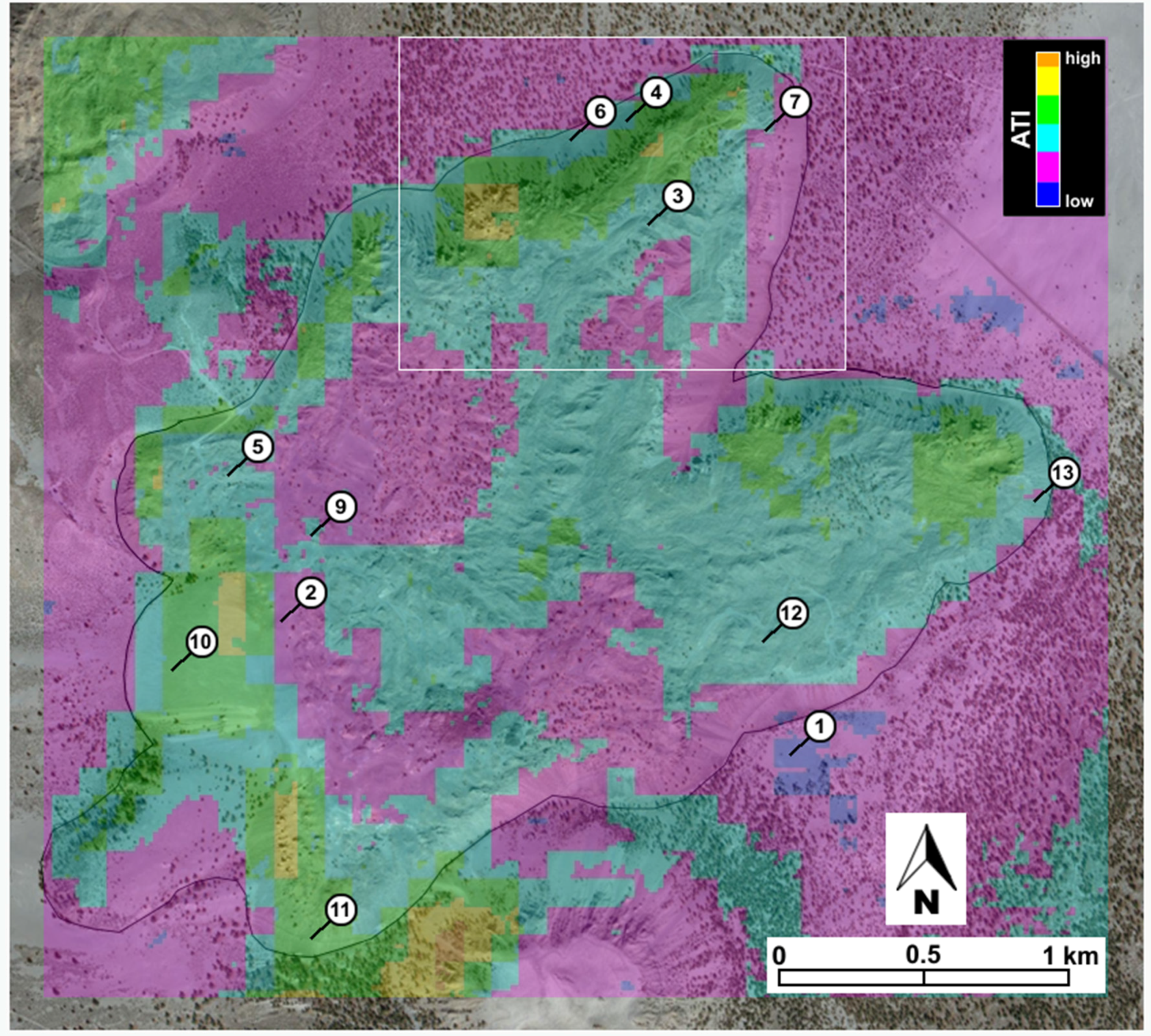
2.4. The Mono Craters and Domes
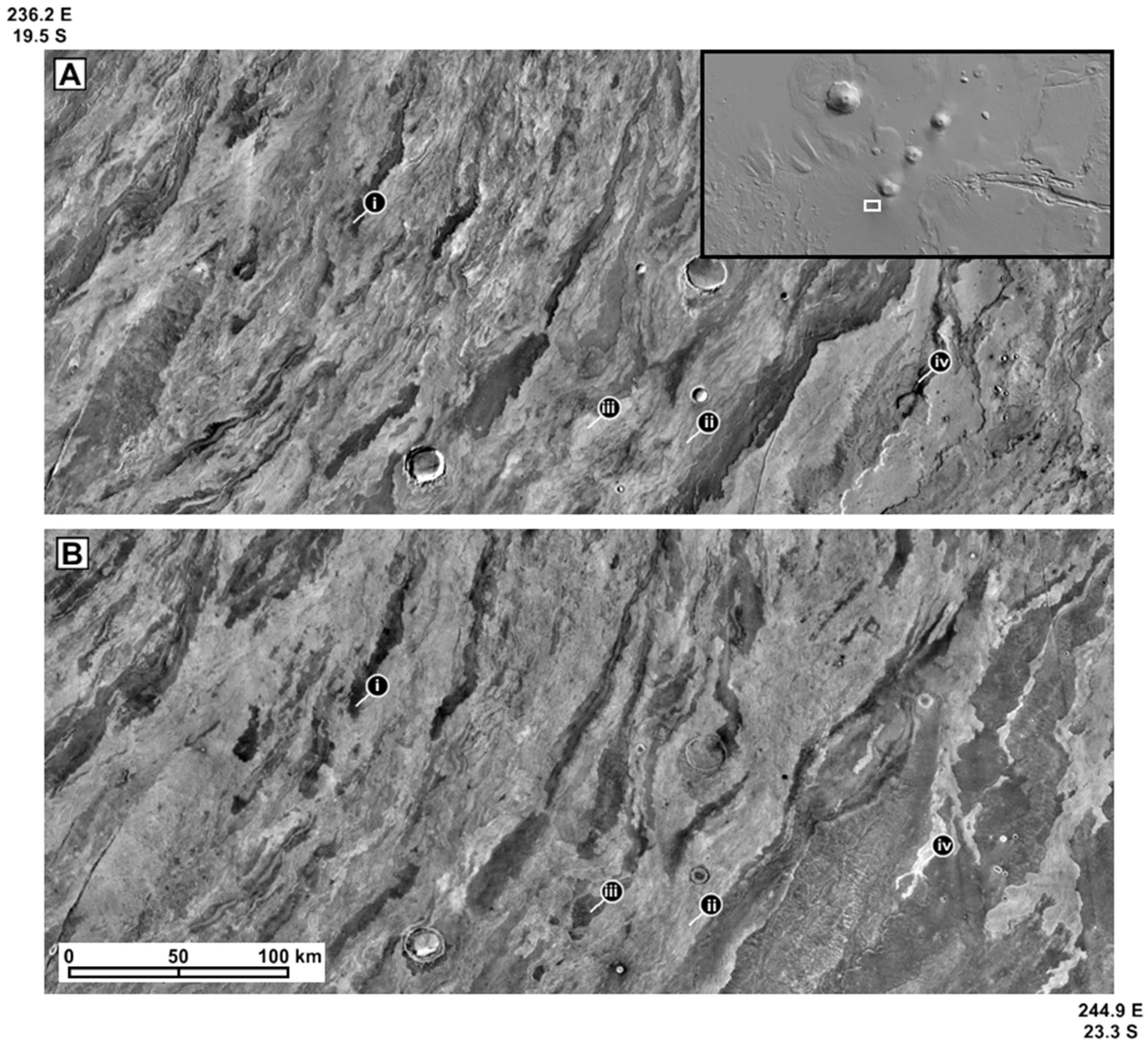
2.5. The Arsia Mons Flow Field
3. Methodology
3.1. ASTER Data Processing
3.2. Field Approach
3.3. Laboratory Analyses
4. Results
4.1. Image Results
4.2. Field Results
4.3. Laboratory Results
4.4. Data Integration
5. Discussion
5.1. Terrestrial Applications
5.2. Applications to Mars
6. Conclusions
Supplementary Materials
Details of Field Approach
Details of Laboratory Analyses
Detailed Results of Field Sites
Acknowledgments
Author Contributions
Conflicts of Interest
References and Notes
- Malin, M.C.; Edgett, K.S. Mars Global Surveyor Mars Orbiter Camera: Interplanetary cruise through primary mission. J. Geophys. Res. 2001, 106, 23429–23570. [Google Scholar] [CrossRef]
- Christensen, P.R.; Bandfield, J.L.; Hamilton, V.E.; Ruff, S.W.; Kieffer, H.H.; Titus, T.N.; Malin, M.C.; Morris, R.V.; Lane, D.M.; Clark, R.N.; et al. Mars Global Surveyor Thermal Emission Spectrometer experiment: Investigation description and surface science results. J. Geophys. Res. 2001, 106, 23823–23871. [Google Scholar] [CrossRef]
- Bandfield, J.L.; Hamilton, V.E.; Christensen, P.R.; McSween, H.Y. Identification of quartzofeldspathic materials on Mars. J. Geophys. Res. 2004, 109. [Google Scholar] [CrossRef]
- Ramsey, M.S.; Crown, D.A. Thermophysical and spectral variability of Arsia Mons lava flows. In Proceedings of the 41st Lunar and Planetary Science Conference, The Woodlands, TX, USA, 1–5 March 2010.
- Hunt, G.R.; Vincent, R.K. The Behavior of Spectral Features in the Infrared Emission from Particulate Surfaces of Various Grain Sizes. J. Geophys. Res. 1968, 73, 6039–6046. [Google Scholar] [CrossRef]
- Mustard, J.F.; Hays, J.E. Effects of hyperfine particles on reflectance spectra from 0.3 to 25 μm. Icarus 1997, 125, 145–163. [Google Scholar] [CrossRef]
- Ramsey, M.S.; Christensen, P.R. Mineral abundance determination: Quantitative deconvolution of thermal emission spectra. J. Geophys. Res. 1998, 103, 577–596. [Google Scholar] [CrossRef]
- Ramsey, M.S.; Fink, J. Estimating silicic lava vesicularity with thermal remote sensing: A new technique for volcanic mapping and monitoring. Bull. Volcanol. 1999, 61, 32–39. [Google Scholar] [CrossRef]
- Scheidt, S.; Ramsey, M.; Lancaste, N. Determining soil moisture and sediment availability at White Sands Dune Field, New Mexico, from apparent thermal inertia data. J. Geophys. Res. 2010, 115. [Google Scholar] [CrossRef]
- Scheidt, S.; Lancaster, N.; Ramsey, M. Eolian dynamics and sediment mixing in the Gran Desierto, Mexico, determined from thermal infrared spectroscopy and remote-sensing data. Geol. Soc. Am. Bull. 2011, 123, 1628–1644. [Google Scholar] [CrossRef]
- Edgett, K.S.; Lancaster, N. Volcaniclastic aeolian dunes: Terrestrial examples and application to Martian sands. J. Arid Environ. 1993, 25, 271–297. [Google Scholar] [CrossRef]
- Fenton, L.K.; Bandfield, J.L. Aeolian processes in Proctor Crater on Mars: Sedimentary history as analyzed from multiple data sets. J. Geophys. Res. 2003, 108. [Google Scholar] [CrossRef]
- Johnson, J.R.; Christensen, P.R.; Lucey, P.G. Dust coatings on basaltic rocks and implications for thermal infrared spectroscopy of Mars. J. Geophys. Res. 2002, 107. [Google Scholar] [CrossRef]
- Ruff, S.W.; Christensen, P.R. Bright and dark regions on Mars: Particle size and mineralogical characteristics based on thermal emission spectrometer data. J. Geophys. Res. 2002, 107. [Google Scholar] [CrossRef]
- Bandfield, J.L. Effects of surface roughness and graybody emissivity on martian thermal infrared spectra. Icarus 2009, 202, 414–428. [Google Scholar] [CrossRef]
- Crown, D.A.; Ramsey, M.S.; Berman, D.C. Morphologic and chronologic studies of lava flow fields in the southern Tharsis region of Mars. In Proceedings of the 43rd Lunar and Planetary Science Conference, The Woodlands, TX, USA, 19–23 March 2012.
- Ramsey, M.S.; Crown, D.A.; Price, M.A. Decoupling lava flow composition and emplacement processes from eolian mantling deposits using thermal infrared data. In Proceedings of the 43rd Lunar and Planetary Science Conference, The Woodlands, TX, USA, 19–23 March 2012.
- Price, M.A.; Ramsey, M.S.; Crown, D.A. Thermophysical characteristics of mantled terrestrial volcanic surfaces: Infrared analogs to the Arsia Mons flows. In Proceedings of the 44th Lunar and Planetary Science Conference, The Woodlands, TX, USA, 18–22 March 2013.
- Crown, D.A.; Ramsey, M.S. Morphologic and thermophysical characteristics of lava flows southwest of Arsia Mons, Mars. J. Volc. Geotherm. Res. 2016. under review. [Google Scholar]
- Hardgrove, C.; Moersch, J.; Whisner, S. Thermal imaging of alluvial fans: A new technique for remote classification of sedimentary features. Earth Planet. Sci. Lett. 2009, 285, 124–130. [Google Scholar] [CrossRef]
- Greeley, R. The Snake River Plain, Idaho: Representative of a new category of volcanism. J. Geophys. Res. 1982, 87, 2705–2712. [Google Scholar] [CrossRef]
- Plescia, J.B. Morphometric properties of martian volcanoes. J. Geophys. Res. 2004, 109. [Google Scholar] [CrossRef]
- Lang, N.P.; Tornabene, L.L.; McSween, H.Y., Jr.; Christensen, P.R. Tharsis-sourced relatively dust-free lavas and their possible relationship to Martian meteorites. J. Volcanol. Geotherm. Res. 2009, 185, 103–115. [Google Scholar] [CrossRef]
- Terra|The EOS Flagship. Available online: terra.nasa.gov (accessed on 7 October 2015).
- Yamaguchi, Y.; Kahle, A.; Tsu, H.; Kawakami, T.; Pniel, M. Overview of Advanced Spaceborne Thermal Emission and Reflectance Radiometer (ASTER). IEEE Trans. Geosci. Remote Sens. 1998, 36, 1062–1071. [Google Scholar] [CrossRef]
- Edgett, K.S.; Malin, M.C. Martian sedimentary rock stratigraphy: Outcrops and interbedded craters of northwest Sinus Meridiani and southwest Arabia Terra. Geophys. Res. Lett. 2002, 29. [Google Scholar] [CrossRef]
- Bandfield, J.L.; Feldman, W.C. Martian high latitude permafrost depth and surface cover thermal inertia distributions. J. Geophys. Res. 2008, 113. [Google Scholar] [CrossRef]
- Price, J.C. Thermal inertia mapping: A new view of the earth. J. Geophys. Res. 1977, 82, 2582–2590. [Google Scholar] [CrossRef]
- Palluconi, F.D.; Kieffer, H.H. Thermal inertia mapping of Mars from 60 S to 60 N. Icarus 1981, 45, 415–426. [Google Scholar] [CrossRef]
- Jakosky, B.M.; Mellon, M.T.; Kieffer, H.H.; Christensen, P.R.; Varnes, E.S.; Lee, S.W. The thermal inertia of Mars from the Mars global surveyor thermal emission spectrometer. J. Geophys. Res. 2000, 105, 9643–9652. [Google Scholar] [CrossRef]
- Fergason, R.L.; Christensen, P.R.; Kieffer, H.H. High-resolution thermal inertia derived from the Thermal Emission Imaging System (THEMIS): Thermal model and applications. J. Geophys. Res. 2006, 111. [Google Scholar] [CrossRef]
- Kieffer, H.H.; Martin, T.Z.; Peterfreund, A.R.; Jakosky, B.M.; Miner, E.D.; Palluconi, F.D. Thermal and albedo mapping of Mars during the Viking primary mission. J. Geophys. Res. 1977, 82, 4249–4291. [Google Scholar] [CrossRef]
- Edgett, K.S.; Christensen, P.R. The particle size of Martian aeolian dunes. J. Geophys. Res. 1991, 96, 22765–22776. [Google Scholar] [CrossRef]
- Christensen, P.R. Martian dust mantling and surface composition: Interpretation of thermophysical properties. J. Geophys. Res. 1982, 87, 9985–9998. [Google Scholar] [CrossRef]
- Fink, J.H.; Manley, C.R. Origin of pumiceous and glassy textures in rhyolite flows and domes. In The Emplacement of Silicic Domes and Lava Flows; Fink, J.H., Ed.; Geological Society of America Special Paper; Geological Society of America: Boulder, CO, USA, 1987; Volume 212, pp. 77–88. [Google Scholar]
- Putzig, N.E.; Mellon, M.T.; Kretke, K.A.; Arvidson, R.E. Global thermal inertia and surface properties of Mars from the MGS mapping mission. Icarus 2005, 173, 325–341. [Google Scholar] [CrossRef]
- Rogers, A.D.; Christensen, P.R.; Bandfield, J.L. Compositional heterogeneity of the ancient Martian crust: Analysis of Ares Vallis bedrock with THEMIS and TES data. J. Geophys. Res. 2005, 110. [Google Scholar] [CrossRef]
- Edwards, C.S.; Bandfield, J.L.; Christensen, P.R.; Fergason, R.L. Global distribution of bedrock exposures on Mars using THEMIS high-resolution thermal inertia. J. Geophys. Res. Planets 2009, 114. [Google Scholar] [CrossRef]
- Van de Griend, A.; Camillo, P.; Gurney, R. Discrimination of soil physical parameters, thermal inertia, and soil moisture from diurnal surf. Water Resour. Res. 1985, 21, 997–1009. [Google Scholar] [CrossRef]
- Rosema, A.; Fiselier, J. Meteosat-based evapotranspiration and thermal inertia mapping for monitoring transgression in the Lake Chad region and Niger Delta. Int. J. Remote Sens. 1990, 11, 741–752. [Google Scholar] [CrossRef]
- Cai, G.; Xue, Y.; Hu, Y.; Wang, Y.; Guo, J.; Luo, Y.; Wu, C.; Zhong, S.; Qi, S. Soil moisture retrieval from MODIS data in Northern China Plain using thermal inertia model. Int. J. Remote Sens. 2007, 28, 3567–3581. [Google Scholar] [CrossRef]
- Matsushima, D.; Kimura, R.; Shinoda, M. A Study on Soil Moisture Estimation using Thermal Inertia. J. Jpn. Soc. Civ. Eng. B1 2012, 67. [Google Scholar] [CrossRef]
- Cracknell, A.P.; Xue, Y. Estimation of ground heat flux using AVHRR data and an advanced thermal inertia model (SoA-TI model). Int. J. Remote Sens. 1996, 17, 637–642. [Google Scholar] [CrossRef]
- Sobrino, J.A.; El Kharraz, M.H. Combining afternoon and morning NOAA satellites for thermal inertia estimation 1: Algorithm and its testing with Hydrologic Atmospheric Pilot Experiment-Sahel data. J. Geophys. Res. 1999, 104, 9445–9453. [Google Scholar] [CrossRef]
- Sobrino, J.A.; El Kharraz, M.H. Combining afternoon and morning NOAA satellites for thermal inertia estimation 2. Methodology and application. J. Geophys. Res. 1999, 104, 9455–9465. [Google Scholar] [CrossRef]
- Price, J.C. On the analysis of thermal infrared imagery: The limited utility of apparent thermal inertia. Remote Sens. Environ. 1985, 18, 59–73. [Google Scholar] [CrossRef]
- Kahle, A.B. Surface emittance, temperature, and thermal inertia derived from Thermal Infrared Multispectral Scanner (TIMS) data for Death Valley, California. Geophysics 1987, 52, 858–874. [Google Scholar] [CrossRef]
- Putzig, N.E.; Mellon, M.T. Apparent thermal inertia and the surface heterogeneity of Mars. Icarus 2007, 191, 68–94. [Google Scholar] [CrossRef]
- Hildreth, W. Volcanological perspectives on Long Valley, Mammoth Mountain, and Mono Craters: Several contiguous but discrete systems. J. Volcanol. Geotherm. Res. 2004, 136, 169–198. [Google Scholar] [CrossRef]
- Bailey, R.A. Geologic Map of Long Valley Caldera, Mono-Inyo Craters Volcanic Chain, and Vicinity, Eastern California; U.S. Geological Survey Map I-1933; U.S. Geological Survey: Reston, VA, USA, 1989.
- Bursik, M.; Sieh, K. Range front faulting and volcanism in the Mono Basin, Eastern California. J. Geophys. Res. 1989, 94, 15587–15609. [Google Scholar] [CrossRef]
- Wood, S. Chronology of Late Pleistocene and Holocene Volcanics, Long Valley and Mono Basin Geothermal Areas, Eastern California; United States Geological Survey Open File Report; U.S. Geological Survey: Reston, VA, USA, 1983.
- Bailey, R.A. Quaternary volcanism of Long Valley Caldera and Mono-Inyo Craters, Eastern California. In Field Trip Guidebook T313; American Geophysical Union: Washington, DC, USA, 1989. [Google Scholar]
- Sieh, K.; Bursik, M. Most recent eruption of the Mono Craters, Eastern Central California. J. Geophys. Res. 1986, 91, 12539–12571. [Google Scholar] [CrossRef]
- Hill, D.P. Response Plan for Volcano Hazards in the Long Valley Caldera and Mono Craters Region, California; U.S. Geological Survey: Reston, VA, USA, 2002; Volume 2185.
- Crumpler, L.S.; Aubele, J.C. Structural evolution of Arsia Mons, Pavonis Mons, and Ascraeus Mons: Tharsis region of Mars. Icarus 1978, 34, 496–511. [Google Scholar] [CrossRef]
- Crumpler, L.S.; Head, J.W.; Aubele, J.C. Calderas on Mars: Characteristics, structure and associated flank deformation. In Volcano Instability on the Earth and Other Planets; McGuire, W.J., Jones, A.P., Neuberg, J., Eds.; Geological Society Special Publication: London, UK, 1996; Volume 110, pp. 307–348. [Google Scholar]
- Head, J.W.; Siebert, N.; Pratt, S.; Smith, D.; Zuber, M.; Solomon, S.; McGovern, P.J.; Garvin, J.B.; The MOLA Science Team. Characterization of major volcanic edifices on Mars using Mars Orbiter Laser Altimeter (MOLA) data. In Proceedings of the 29th Lunar and Planetary Science Conference, The Woodlands, TX, USA, 16–20 March 1998.
- Head, J.W.; Siebert, N.; Pratt, S.; Smith, D.; Zuber, M.; Garvin, J.B.; McGovern, P.J.; The MOLA Science Team. Volcanic calderas on Mars: Initial views using Mars Orbiter Laser Altimeter (MOLA) data. In Proceedings of the 29th Lunar and Planetary Science Conference, The Woodlands, TX, USA, 16–20 March 1998.
- Mouginis-Mark, P.J. Prodigious ash deposits near the summit of Arsia Mons volcano, Mars. Geophys. Res. Lett. 2002, 29. [Google Scholar] [CrossRef]
- Scott, D.; Zimbelman, J. Geologic Map of Arsia Mons Volcano, Mars; U.S. Geological Survey Miscellaneous Investigation Series Map I-2480; U.S. Geological Survey: Reston, VA, USA, 1995.
- Ramsey, M.S.; Crown, D.A. Mantled lava flow surfaces on Earth: Thermo-physical analogs for Martian volcanism? In Proceedings of the American Geophysical Union, Fall Meeting, San Francisco, CA, USA, 5–9 December 2011.
- Scott, D. Map Showing Lava Flows in the Southeast Part of the Phoenicis Lacus Quadrangle of Mars; U.S. Geological Survey Miscellaneous Investigation Series Map I-1274; U.S. Geological Survey: Reston, VA, USA, 1981.
- Scott, D.; Schaber, G.; Dial, A. Map Showing Lava Flows in the Southwest Part of the Phoenicis Lacus Quadrangle of Mars; U.S. Geological Survey Miscellaneous Investigation Series Map I-1275; U.S. Geological Survey: Reston, VA, USA, 1981.
- Scott, D.; Schaber, G.; Horstman, K.; Dial, A.; Tanaka, K. Map Showing Lava Flows in the Northwest Part of the Phoenicis Lacus Quadrangle of Mars; U.S. Geological Survey Miscellaneous Investigation Series Map I-1272; U.S. Geological Survey: Reston, VA, USA, 1981.
- Bleacher, J.E.; Greeley, R.; Williams, D.A.; Cave, S.R.; Neukum, G. Trends in effusive style at the Tharsis Montes, Mars, and implications for the development of the Tharsis province. J. Geophys. Res. 2007, 112. [Google Scholar] [CrossRef]
- Garry, W.B.; Williams, D.A.; Bleacher, J.E.; Dapremont, A.M. Geologic mapping of Olympus Mons and Tharsis Montes, Mars. In Proceedings of the 46th Lunar and Planetary Science Conference, The Woodlands, TX, USA, 16–20 March 2015.
- Russell, I.C. Quaternary History of the Mono Valley, California; U.S. Geological Survey Eighth Annual Report; U.S. Geological Survey: Reston, VA, USA, 1889; pp. 267–394.
- National Climatic Data Center (NCDC). NOAA, n.d. Web. 24 March 2013.
- Google Earth. 37°53′42.34″ N, 119°0′16.07″ W. Available online: https://www.google.com/earth/ (accessed on 15 November 2012).
- Abrams, M. The Advanced Spaceborne Thermal Emission and Reflection Radiometer (ASTER): Data products for the high spatial resolution imager on NASA’s Terra platform. Int. J. Remote Sens. 2000, 21, 847–859. [Google Scholar] [CrossRef]
- Realmuto, V.J. Separating the effects of temperature and emissivity: Emissivity spectrum normalization. In Proceedings of the 2nd TIMS Workshop, Pasadena, CA, USA, 6 June 1990; Jet Propulsion Laboratory Publication: Pasadena, CA, USA, 1990; pp. 90–155. [Google Scholar]
- Ramsey, M.S.; Fink, J.H. Estimating lava vesicularity: A new technique using thermal infrared remote sensing data. Am. Geophys. Union Eos Trans. 1996, 77, F803. [Google Scholar]
- Mars, J.C.; Rowan, L.C. Spectral assessment of new ASTER SWIR surface reflectance data products for spectroscopic mapping of rocks and minerals. Remote Sens. Environ. 2010, 114, 2011–2025. [Google Scholar] [CrossRef]
- Lee, R.J.; King, P.L.; Ramsey, M.S. Spectral analysis of synthetic quartzofeldspathic glasses using laboratory thermal infrared spectroscopic methods. J. Geophys. Res. 2010, 115. [Google Scholar] [CrossRef]
- Simurda, C.M.; Ramsey, M.S. Correcting topographic shadowing errors in apparent thermal inertia images. In Proceedings of the 45th Lunar and Planetary Science Conference, The Woodlands, TX, USA, 17–21 March 2014.
- Anderson, S.W.; Stofan, E.R.; Plaut, J.J.; Crown, D.A. Block size distributions on silicic lava flow surfaces: Implications for emplacement conditions. Geol. Soc. Am. Bull. 1998, 110, 1258–1267. [Google Scholar] [CrossRef]
- Vaughan, R.A. (Ed.) Remote Sensing Applications in Meteorology and Climatology; Springer Science & Business Media: Berlin, Germany, 1987; Volume 201.
- Mellon, M.T.; Jakosky, B.M.; Kieffer, H.H.; Christensen, P.R. High-resolution thermal inertia mapping from the Mars global surveyor thermal emission spectrometer. Icarus 2000, 148, 437–455. [Google Scholar] [CrossRef]
- Ruff, S.W.; Christensen, P.R.; Barbera, P.W.; Anderson, D.L. Quantitative thermal emission spectroscopy of minerals: A laboratory technique for measurement and calibration. J. Geophys. Res. 1997, 102, 14899–14913. [Google Scholar] [CrossRef]


| Bridgeport, CA | Sonora Junction, CA | ||
|---|---|---|---|
| Elevation: | Location: | Elevation: | Location: |
| 598.4 m | 38.25°N, 119.22°W | 639.7 m | 38.4°N, 199.5°W |
| Date | Precipitation (cm) | Date | Precipitation (cm) |
| 28 June 2011 | 0 | 28 June 2011 | 1.02 |
| 29 June 2011 | 0 | 29 June 2011 | 0 |
| 30 June 2011 | 0 | 30 June 2011 | 0 |
| 1 July 2011 | trace | 1 July 2011 | trace |
| 2 July 2011 | 0 | 2 July 2011 | 0 |
| 3 July 2011 | 0 | 3 July 2011 | 0 |
| 4 July 2011 | 0 | 4 July 2011 | 0 |
| 5 July 2011 | 0 | 5 July 2011 | 0 |
| 6 July 2011 | 0 | 6 July 2011 | 0 |
| 7 July 2011 | 0 | 7 July 2011 | 0 |
| 8 July 2011 | 0 | 8 July 2011 | 0 |
| 9 July 2011 | 0 | 9 July 2011 | 0 |
| 10 July 2011 | 0 | 10 July 2011 | 0 |
| 11 July 2011 | 0 | 11 July 2011 | 0 |
| 12 July 2011 | 0 | 12 July 2011 | 0 |
| 13 July 2011 | 0 | 13 July 2011 | 0 |
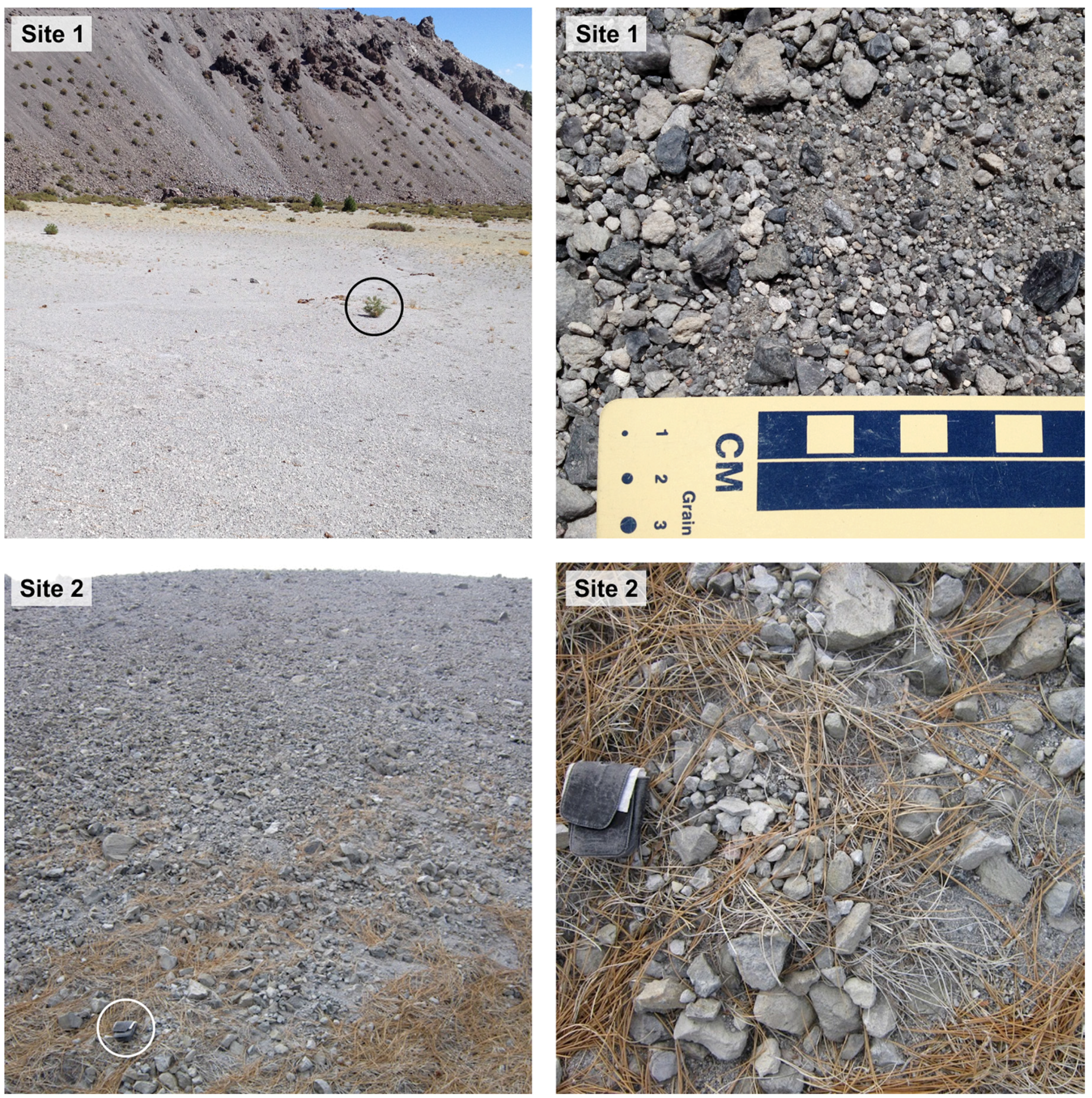
| Site 1 | |
| Average fragment size (cm): | 0.5–1.0 |
| Mantling depth (cm): | 8.0–16.0 |
| ATI value (×100): | 1.960 |
| General composition: | rhyolitic (80% pumice/20% obsidian) |
| Sorting degree: | well-sorted |
| Surface temperature (°C): | 17.0 |
| Local time: | 10:15 a.m. |
| Field description: | Course, angular grains, sand to gravel-sized. Well-sorted. |
| Site 2 | |
| Average fragment size (cm): | 1.0–2.0 |
| Mantling depth (cm): | <10 |
| ATI value (×100): | 2.317 |
| General composition: | rhyolitic |
| Sorting degree: | moderately-sorted |
| Surface temperature (°C): | 30.0 |
| Local time: | 15:00 p.m. |
| Field description: | Well-sorted pyroclastic deposits. Course, angular, sand to gravel-sized grains. Predominantly pumice in composition. |
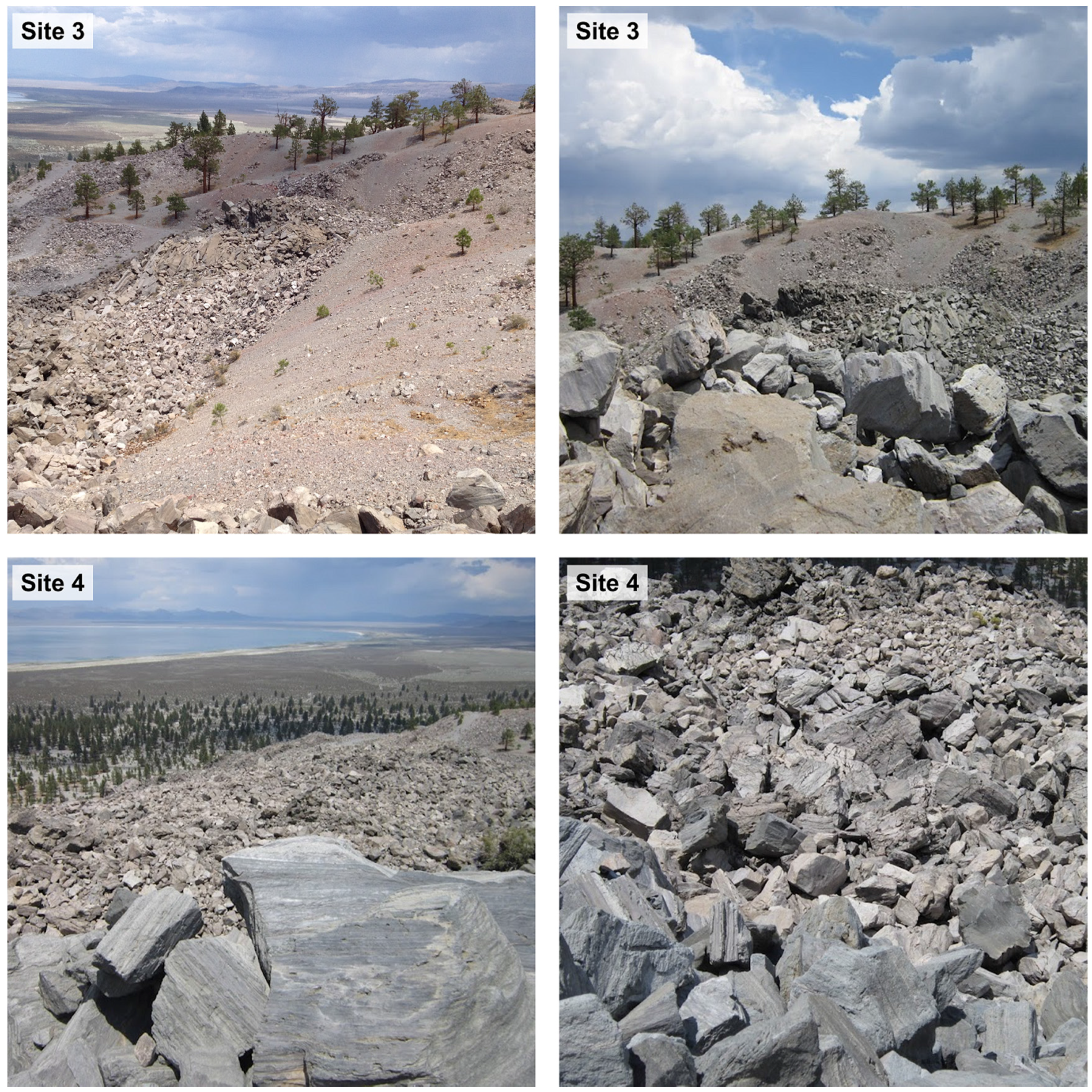
| Site 3 | |
| Average fragment size (cm): | bimodal (0.03 and 0.50) |
| Mantling depth (cm): | not measured (inaccessible) |
| ATI value (×100): | 2.576 |
| General composition: | rhyolitic |
| Sorting degree: | very poorly sorted |
| Surface temperature (°C): | not measured (inaccessible) |
| Local time: | n/a |
| Field description: | Poorly-sorted mixture of pumice, obsidian, and other dome rocks. Large variation in size, from small sand-sized grains to 0.5m blocks. |
| Site 4 | |
| Average fragment size (cm): | 40.0 |
| Mantling depth (cm): | 0.0 |
| ATI value (×100): | 2.860 |
| General composition: | rhyolitic (pumice and obsidian boulders) |
| Sorting degree: | well-sorted |
| Surface temperature (°C): | not measured |
| Local time: | n/a |
| Field description: | Well-sorted large volcanic debris consisting of pumice obsidian, and other dome rocks. Large, angular blocks ~1 m. |
| Site 5 | |
| Average fragment size (cm): | <0.5 |
| Mantling depth (cm): | <30 |
| ATI value (×100): | 2.645 |
| General composition: | rhyolitic |
| Sorting degree: | well-sorted |
| Surface temperature (°C): | 46.2 |
| Local time: | ~2:00 p.m. |
| Field description: | Well-sorted pumice dune consisting of fine sand. Wind-deposited. Surrounded by slopes of larger volcanic fragments. |
| Site 6 | |
| Average fragment size (cm): | 3.0–6.0 |
| Mantling depth (cm): | none |
| ATI value (×100): | 2.850 |
| General composition: | rhyoltic |
| Sorting degree: | poorly-sorted |
| Surface temperature (°C): | n/a |
| Local time: | n/a |
| Field description: | Poorly-sorted weathered slope debris. Fragments range from smaller rocks a few cm in diameter to large meter-sized boulders. Minimal mantling. |
| Site 7 | |
| Average fragment size (cm): | 1.0–3.0 |
| Mantling depth (cm): | 20.0 |
| ATI value (×100): | 2.777 |
| General composition: | rhyolitic (pumice and obsidian boulders) |
| Sorting degree: | poorly-sorted |
| Surface temperature (°C): | not measured |
| Local time: | n/a |
| Field description: | Poorly-sorted sand- and gravel-sized grains. About 30% is rhyolitic pumice boulders. Average boulder size ~0.3 m. |
| Site 8 | |
| Average fragment size (cm): | 4.0 |
| Mantling depth (cm): | none |
| ATI value (×100): | 2.461 |
| General composition: | rhyolitic |
| Sorting degree: | poorly-sorted |
| Surface temperature (°C): | n/a |
| Local time: | n/a |
| Field description: | Poorly-sorted debris weathered off the east slope. 70% pumice 30% obsidian. Most fragments ~3–5 cm in size. Larger fragments ~15–20 cm. |
| Site 9 | |
| Average fragment size (cm): | 1.0 |
| Mantling depth (cm): | n/a |
| ATI value (×100): | 2.555 |
| General composition: | rhyolitic |
| Sorting degree: | well-sorted |
| Surface temperature (°C): | n/a |
| Local time: | n/a |
| Field description: | Well-sorted wind-deposited pumice sediment. Some outcrops of larger volcanic debris. |
| Site 10 | |
| Average fragment size (cm): | <3 |
| Mantling depth (cm): | None |
| ATI value (×100): | 2.731 |
| General composition: | rhyolitic (pumice boulders) |
| Sorting degree: | Intermediate |
| Surface temperature (°C): | 22.5 |
| Local time: | n/a |
| Field description: | Slope with larger pumice fragments. Weathering of fragments varied. 80% pumice and 20% obsidian. Average grain size ~3 cm, varied. |
| Site 11 | |
| Average fragment size (cm): | 0.5 |
| Mantling depth (cm): | <30 |
| ATI value (×100): | 3.340 |
| General composition: | rhyolitic (90% pumice/10% obsidian) |
| Sorting degree: | well-sorted |
| Surface temperature (°C): | 55.7 |
| Local time: | 11:45 a.m. |
| Field description: | Very well sorted rhyolitic grains. Some obsidian grains. High ATI value probably the result of sun angle/shadowing on western slopes. |
| Site 12 | |
| Average fragment size (cm): | 40.0 |
| Mantling depth (cm): | None |
| ATI value (×100): | 2.943 |
| General composition: | rhyolitic (pumice and obsidian boulders) |
| Sorting degree: | well-sorted |
| Surface temperature (°C): | not measured |
| Local time: | n/a |
| Field description: | Well-sorted rhyolitic boulders with minimal mantling. |
| Site 13 | |
| Average fragment size (cm): | 4.0–6.0 |
| Mantling depth (cm): | n/a |
| ATI value (×100): | 2.697 |
| General composition: | rhyolitic (70% pumice/30% obsidian) |
| Sorting degree: | poorly-sorted |
| Surface temperature (°C): | 22.5 |
| Local time: | 9:00 a.m. |
| Field description: | Poorly sorted slope debris. All grains and blocks very angular. Debris ranges from fine sand to >0.3 m fragments. |
© 2016 by the authors; licensee MDPI, Basel, Switzerland. This article is an open access article distributed under the terms and conditions of the Creative Commons by Attribution (CC-BY) license (http://creativecommons.org/licenses/by/4.0/).
Share and Cite
Price, M.A.; Ramsey, M.S.; Crown, D.A. Satellite-Based Thermophysical Analysis of Volcaniclastic Deposits: A Terrestrial Analog for Mantled Lava Flows on Mars. Remote Sens. 2016, 8, 152. https://doi.org/10.3390/rs8020152
Price MA, Ramsey MS, Crown DA. Satellite-Based Thermophysical Analysis of Volcaniclastic Deposits: A Terrestrial Analog for Mantled Lava Flows on Mars. Remote Sensing. 2016; 8(2):152. https://doi.org/10.3390/rs8020152
Chicago/Turabian StylePrice, Mark A., Michael S. Ramsey, and David A. Crown. 2016. "Satellite-Based Thermophysical Analysis of Volcaniclastic Deposits: A Terrestrial Analog for Mantled Lava Flows on Mars" Remote Sensing 8, no. 2: 152. https://doi.org/10.3390/rs8020152