ℓ₀-Norm Sparse Hyperspectral Unmixing Using Arctan Smoothing

Abstract

The goal of sparse linear hyperspectral unmixing is to determine a scanty subset of spectral signatures of materials contained in each mixed pixel and to estimate their fractional abundances. This turns into an ${\ell }_0$-norm minimization, which is an NP-hard problem. In this paper, we propose a new iterative method, which starts as an ${\ell }_1$-norm optimization that is convex, has a unique solution, converges quickly and iteratively tends to be an ${\ell }_0$-norm problem. More specifically, we employ the arctan function with the parameter $\sigma \ge 0$ in our optimization. This function is Lipschitz continuous and approximates ${\ell }_1$-norm and ${\ell }_0$-norm for small and large values of σ, respectively. We prove that the set of local optima of our problem is continuous versus σ. Thus, by a gradual increase of σ in each iteration, we may avoid being trapped in a suboptimal solution. We propose to use the alternating direction method of multipliers (ADMM) for our minimization problem iteratively while increasing σ exponentially. Our evaluations reveal the superiorities and shortcomings of the proposed method compared to several state-of-the-art methods. We consider such evaluations in different experiments over both synthetic and real hyperspectral data, and the results of our proposed methods reveal the sparsest estimated abundances compared to other competitive algorithms for the subimage of AVIRIS cuprite data.

1. Introduction

Hyperspectral remote sensing has a wide range of applications, from food quality inspection to military functions [1,2,3,4,5,6]. The hyperspectral imaging data are collected by means of hyperspectral imaging sensors and contain two-dimensional spatial images over many contiguous bands of high spectral resolution [3,4]. Along with the observed pure pixels, the mixed pixels can occur because of the relatively low spatial resolution of the sensor flying at high altitudes, as well as the combination of distinct materials form intimate mixtures. Thus, spectral unmixing (SU) is required to characterize the measured pixels recorded by remote sensors. Following the unmixing process, we can consider two types of mixing models, including the linear mixing model (LMM) and non-linear mixing. Although the linear unmixing methods for the former models are the most common techniques in hyperspectral unmixing methods, the latter model also causes one to investigate an alternative unmixing procedure to overcome the inherent restrictions of the linear model, called nonlinear SU. These model indeed may happen in some applicable scenarios in which multiple scattering is emitted from different materials. In some environments, such as urban scenes [7], vegetation areas [8] and those containing specific spectral signatures, such as soil, sand and trees [9,10], we have to use the nonlinear mixing model. However, the linear SU methods are being scrutinized by researchers and scientists extensively because of their capabilities in many applications [4,5,11,12,13], e.g., minerals [4,14]. In this paper, we focus on the linear SU, which is a method of the separation of the mixed pixel spectrum into a set of the spectral signatures of the materials called endmembers, as well as their corresponding contributions in each mixed pixel called abundances in a linear fashion.

Since the number of endmembers/materials present at each mixed pixel is normally scanty compared to the number of total endmembers in most applications, we can consider the problem of SU as a sparse unmixing problem [15,16,17,18,19,20,21,22,23]. Mathematically, the corresponding sparse problem is an ${\ell }_0$-norm problem and is an NP-hard problem due to the required exhaustive combinatorial search [24,25]. Indeed, the fractions of endmembers in each mixed pixel can be determined by solving a minimization problem containing an objective function that counts the nonzero components of the vector of fractional abundances of endmembers under a reasonable error coming from the modelling type, as well as measurement errors. In a practical scenario, two more constraints can be imposed on this problem because of the physical considerations, which are (1) the sum of the fractional abundances is one and (2) they are nonnegative.

In recent years, several approximation methods have been proposed for the ${\ell }_0$-norm minimization problem notwithstanding various unmixing methods, which employed ${\ell }_1$-norm instead of ${\ell }_0$-norm (e.g., [17,19,22,26]). These may include iterative reweighted schemes (e.g., [27,28]), greedy algorithms [29,30], Bayesian learning algorithms [18], ${\ell }_q$ regularization [31] and compressive sensing schemes [21,32]. Each of these methods has specific characteristics, e.g., the method proposed in [18] exploits Bayesian learning to control the parameters involved. Some algorithms have used better approximations of the ${\ell }_0$-norm, e.g., the ${\ell }_p$-norm is approximated as a weighted $l_2$-norm in [33]. Although these methods improve the sparsity, the ${\ell }_p$-norm function is not Lipschitz continuous for $p<1$. As a result, these methods suffer from numerical problems for smaller values of p. Thus, an attractive solution is to employ Lipschitz continuous approximations, such as the exponential function, the logarithm function or sigmoid functions, e.g., [20,23,34]. The arctan function is also used in different literature works for sparse regularization, such as approximating the sign function appearing in the derivative of the ${\ell }_1$-norm term in [35], introducing a penalty function for the sparse signal estimation by the maximally-sparse convex approach in [36] or approximating the ${\ell }_0$-norm term through a weighted ${\ell }_1$-norm term in [23].

In this paper, we propose a new algorithm utilizing an arctan function, which allows us to start our search with the ${\ell }_1$-norm problem, which is convex and initially guarantees fast convergence to the unique optimal solution. This method allows us to iteratively update our problem to better approximate the ${\ell }_1$-norm problem and provides an enhanced separation of the zero components. The proposed arctan sum is a smooth approximation of the ${\ell }_0$-norm and ${\ell }_1$-norm as a function of σ. We gradually increase the parameter σ in order to allow the convergence and tracking of the best local optimal solution and iteratively find a better sparse solution. The arctan function is Lipschitz continuous; thus, the proposed method does not have additional considerations to avoid numerical problems, e.g., [25,37,38]. Moreover, our proposed algorithm improves the sparsity as σ varies from zero to ∞, whereas in [20,23], the value of σ is constant. We use the alternating direction method of multipliers (ADMM) to minimize the resulting objective function at each iteration [39,40]. We prove that the set of local optima of our objective function is continuous with the Hausdorff metric versus σ. This implies that iterative minimization along with a gradual increase of σ guarantees the convergence to the optimal solution. Finding the appropriate increasing sequence for σ is an open problem to guarantee this convergence and to reduce the number of iterations. Thus, we simply propose to increase σ exponentially. We compare our proposed method to several state-of-the-art methods [17,18,26,33] over both the synthetic data and real hyperspectral data. Our results show that our method results in a higher reconstruction signal-to-noise ratio (RSNR) for the fractional abundances than some state-of-the-art methods and outperforms them in the sense of the probability of success (PoS), except for the SUnSAL (sparse unmixing by variable splitting and augmented Lagrangian) method [17,26].

The remainder of the paper is organized as follows. The sparse spectral unmixing is formulated in Section 2. The arctan function is proposed in Section 3, leading to our unmixing algorithm. The proposed method is compared to several state-of-the-art methods via simulations in Section 4. Finally, we conclude the paper in Section 5.

2. Sparse Spectral Unmixing

In this section, after reviewing the linear mixing model (LMM), which is applicable for many scenarios for the hyperspectral unmixing, we briefly provide the sparse hyperspectral unmixing through the ${\ell }_0$-norm problem.

In the LMM, the measured spectra for the pixels of the scene, which are composed of the linear combination of the spectral signatures scattered from the materials and their fractions, can be formulated by:

$$\mathbf{y}=\Phi \mathbf{x}+\mathbf{n},$$

(1)

where $\mathbf{y}\in {\mathbb{R}}^L$ represents the measured mixed pixel, $\Phi \in {\mathbb{R}}_{+}^{L\times q}$ is the spectral signatures’ library containing q pure spectral signatures and L spectral bands, $\mathbf{x}\in {\mathbb{R}}_{+}^q$ is the corresponding fractions of abundances for each endmember, ${\mathbb{R}}_{+}$ is the set of non-negative real numbers and $\mathbf{n}\in {\mathbb{R}}^L$ is an additive noise vector. There are two constraints for the fractional abundance vector $\mathbf{x}$ in the LMM as the abundance nonnegativity constraint (ANC), $0\le x_i\le 1,i=1,2,\cdots ,q$, and abundance sum-to-one constraint (ASC), ${\mathbf{1}}^T\mathbf{x}={\sum }_{i=1}^q{x}_i=1$, where ${\mathbf{1}}^T$ is the transposed column vector of ones. It should be noted that the ASC is not explicitly imposed in the problem for some scenarios, since it is prone to strong criticism, e.g., see [22,35,41] and the references therein. However, these constraints provide an enhanced and reliable result for the estimated fractional abundances in the linear spectral mixture analysis [42], and we consider both constraints in our formulation, as many unmixing methods include the state-of-the-art methods in this manuscript consider these constraints, as well.

In a sparse linear hyperspectral unmixing process, it is assumed that the spectral signatures of endmembers are chosen from a large number of spectral samples of the spectral library available a priori, e.g., [4,17]. Besides, one can assume that the number of spectral signatures contributed in the measured hyperspectral data cube is much smaller than the dimension of the spectral library (e.g., typically less than six [4,5]). Thus, we can consider the problem of SU as a sparse unmixing problem to determine the fractional abundance vector $\mathbf{x}$ as the following constraint ${\ell }_0$-norm problem:

$$\begin{array}{ccc}\hfill \underset{\mathbf{x}\in \mathbb{S}}{min}{\left|\right|\mathbf{x}\left|\right|}_0& \mathrm{subject}\mathrm{to}& \left|\right|\mathbf{y}-{\Phi \mathbf{x}\left|\right|}_2^2\le ϵ,\hfill \end{array}$$

(2)

where ${\left|\right|\mathbf{x}\left|\right|}_0$ shows its nonzero components, ϵ is a small positive value and the polytope $\mathbb{S}$, which is a $q-1$ standard simplex, contains both ANC and ASC constraints.

Finding the optimal solution of Equation (2) is an NP-hard [43], i.e., various subsets of the endmembers that are possibly present must be verified for each mixed pixel from a given spectral library. As a remedy, several efficient linear sparse techniques are proposed for the unmixing process, e.g., [4,5,17,18,26]. Minimizing the ${\ell }_1$-norm as approximation instead of the ${\ell }_0$-norm is one of the earliest methods proposed to avoid an exhaustive search for Equation (2) (e.g., see [44,45] and the references therein; see also [17,22,26,35,41,46,47] for unmixing techniques), as follows:

$$\begin{array}{ccc}\hfill \underset{\mathbf{x}\in \mathbb{S}}{min}{\left|\right|\mathbf{Wx}\left|\right|}_1& \mathrm{subject}\mathrm{to}& \left|\right|\mathbf{y}-{\Phi \mathbf{x}\left|\right|}_2^2\le ϵ,\hfill \end{array}$$

(3)

where ${\left|\right|\mathbf{Wx}\left|\right|}_1={\sum }_{i=1}^q{w}_i\left|x_i\right|$ is a weighted ${\ell }_1$-norm of $\mathbf{x}$, $\mathbf{W}$ is a diagonal matrix and $w_i$’s are its diagonal entries. In [17,22,26,41], the above problem is considered using $\mathbf{W}=\mathbf{I}$. Alternative weighting matrices are employed in [46,47].

Many researchers have proposed the use of the ${\ell }_p$-norm for $p<1$ as a better approximation for the ${\ell }_0$-norm, e.g., [33,38,48,49]. Smaller values of p result in better approximation; however, they result in an increase in the number of local optima, which either trap the algorithms in a suboptimal solution or translate into increased computational complexity. An alternative method is to iteratively reduce p from one to zero in order to take advantage of the unique optimal solution for $p=1$ and then track the optimal solution for $p<1$ as p is reducing [38]. The existing methods using the ${\ell }_p$-norm have a major drawback since for $p<1$, the ${\ell }_p$-norm is not a Lipschitz continuous function. In fact, these methods must introduce an extra parameter to make it Lipschitz continuous, which leads to more approximations. In this paper, we propose to employ the arctan function as a robust approximation that is Lipschitz continuous. This method allows an accurate approximation of the problem starting with the ${\ell }_1$-norm and iteratively converging to the ${\ell }_0$-norm.

To the best of our knowledge, two kinds of smoothing ${\ell }_0$-norm minimization problems were used for the spectral unmixing application. An iterative weighted algorithm based on the logarithm smoothed function was proposed in [20]. Later, another method was proposed in [23] that utilized the arctan function for approximating the ${\ell }_0$-norm term. In these methods, a constant parameter σ allows one to control the sparsity of the solution. In [23], a fixed arctan function is used to approximate the ${\ell }_0$-norm without any guarantee if an enhanced solution can be tracked. However in this paper, we propose to iteratively enhance the employed approximation function in order to avoid the algorithm being trapped in local minima. In contrast to [23], the approximation error of the ${\ell }_0$-norm tends to zero iteratively. This arctan approximation initially equals the ${\ell }_1$-norm and modifies it to the ${\ell }_0$-norm iteratively, discussed in the next section. To show that the set of optimal candidate solutions is a continuous function in terms of σ, we prove Theorem 1, where it gives this insight to move from a unique solution at the starting point and iteratively directs to the closest solution to the ${\ell }_0$-norm.

3. Our Proposed Unmixing Method: Arctan Approximation of the ${\ell }_1$- and ${\ell }_0$-Norms

We propose the following function to approximate the ${\ell }_1$ or ${\ell }_0$-norms

$$\begin{array}{c}\hfill F(\sigma ,\mathbf{x})=g(\sigma )\sum _{i=1}^{q}arctan(\sigma x_i),\end{array}$$

(4)

where $\sigma >0$ is a tunable parameter and $0\le x_i\le 1$. We find an appropriate function for $g(\sigma )$, such that $F(\sigma ,\mathbf{x})$ converges to the ${\ell }_1$ and ${\ell }_0$-norms, respectively, as σ tends to zero and ∞. The basic idea behind this concept is to start at $\sigma =0$ for which our problem becomes the ${\ell }_1$-norm problem in Equation (3). Thus, the problem becomes a convex optimization for $\sigma =0$ that is known to be a good approximation of Equation (2) [50] . By iteratively increasing σ, the proposed problem-minimizing Equation (4) tends to the problem in Equation (2).

Remark 1. 

We shall choose $g(\sigma )$, such that the following conditions are satisfied:

(i) 

$F(\sigma ,\mathbf{x})$ tends to ${\left|\right|\mathbf{x}\left|\right|}_1$ as σ tends to zero.

(ii) 

$F(\sigma ,\mathbf{x})$ tends to ${\left|\right|\mathbf{x}\left|\right|}_0$ as σ tends to ∞.

There are many such functions that satisfy the above conditions, such as follows:

$$\begin{array}{c}\hfill g_1(\sigma )=\frac{2}{\pi }+\frac{1}{\sigma },\end{array}$$

(5)

$$\begin{array}{c}\hfill g_2(\sigma )=\frac{1}{arctan(\sigma )},\end{array}$$

(6)

where $\sigma >0$.

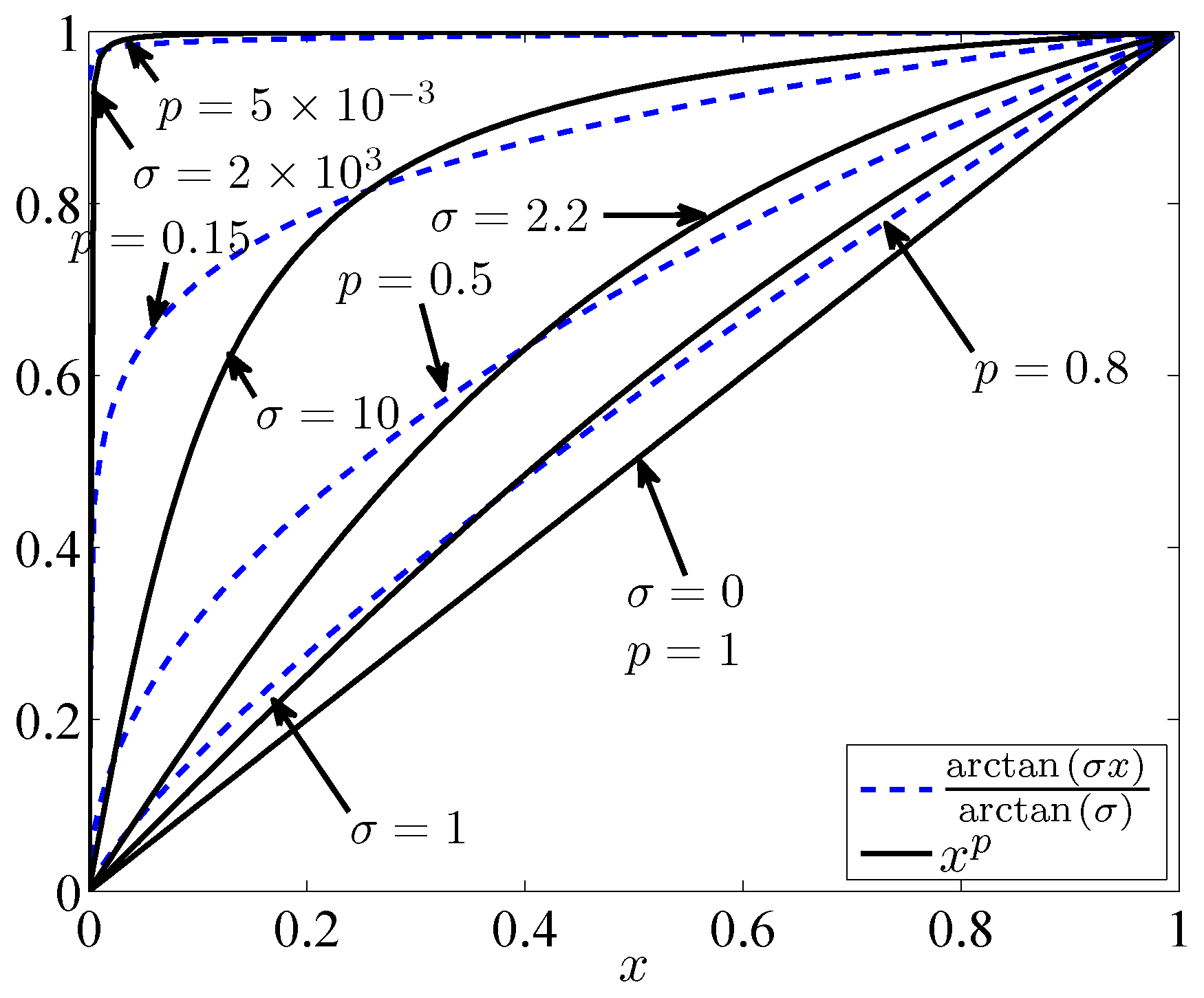
Figure 1 shows the curves of functions $\frac{arctan(\sigma x)}{arctan(\sigma )}$ and $x^p$ for $x\in [0,1]$ and several different values of σ and p. We see that for $p=1$ and $\sigma \to 0$, these functions become linear, and both yield the ${\ell }_1$-norm. As $p\to 0$ and $\sigma \to \infty$, these functions tend to the unit step function and both yield the ${\ell }_0$-norm. For values of p between one and zero and σ between zero and ∞, we observe that these curves are similar and that they can approximate each other. However, the important difference between these functions is in their derivatives for small values of x around zero; in contrast to $\frac{arctan(\sigma x)}{arctan(\sigma )}$, the derivatives of $x^p$ are not bounded around $x=0$. These unbounded derivatives cause numerical instabilities in iterative algorithms.

The approximation of the ${\ell }_0$-norm problem using the function $F(\sigma ,\mathbf{x})$ for the constrained ${\ell }_0$-norm problem can be considered as follows:

$$\begin{array}{ccc}\hfill \underset{\mathbf{x}\in \mathbb{S}}{min}F(\sigma ,\mathbf{x})& \mathrm{subject}\mathrm{to}& \left|\right|\mathbf{y}-{\Phi \mathbf{x}\left|\right|}_2^2\le ϵ,\hfill \end{array}$$

(7)

as σ increases. The unconstrained version of Equation (7) using the Lagrangian method can be presented by:

$$\begin{array}{cc}\hfill & \underset{\mathbf{x}\in \mathbb{S}}{min}f(\mathbf{x},\sigma ),\hfill \end{array}$$

(8)

$$\begin{array}{cc}\hfill & f(\mathbf{x},\sigma )=\frac{1}{2}\left|\right|\mathbf{y}-{\Phi \mathbf{x}\left|\right|}_2^2+\lambda g(\sigma )\sum _{i=1}^{q}arctan(\sigma x_i),\hfill \end{array}$$

(9)

where there exists some $\lambda >0$, such that Equation (7) and Equation (8) are equivalent.

Now, we prove the continuity of the set of candidate local minima of Equation (8) with respect to the parameter σ to guarantee that our proposed method reaches the possible sparse solution (i.e. if it exists) while σ is varying. The motivation behind Theorem 1 is to give insight to the solution obtained using the previous value of σ as a good initialization for the next iteration with the larger value of σ.

Using the definition of Hausdorff distance mentioned in Appendix A, the following theorem proves the desired continuity of the set of all candidate local minima.

Theorem 1. 

Let ${\mathbf{X}}_{\sigma }\subset \mathcal{X}$ be the set of all solutions of:

$$\begin{array}{c}\hfill {\nabla }_{\mathbf{x}}f(\mathbf{x},\sigma )=\lambda \mathbf{v}(\mathbf{x},\sigma )+{\Phi }^T\Phi \mathbf{x}-{\Phi }^T\mathbf{y}=0,\end{array}$$

(10)

where $\mathbf{v}(\mathbf{x},\sigma )={[\frac{\sigma g(\sigma )}{1+{\sigma }^2{x}_1^2},...,\frac{\sigma g(\sigma )}{1+{\sigma }^2{x}_q^2}]}^T$. Then, ${\mathbf{X}}_{\sigma }$ is a continuous function of $\sigma \in [0,\infty )$.

Proof. 

See Appendix A. ☐

For simplicity, the above theorem is written for the simplified case where $\mathbb{S}$ is relaxed into ${\mathbb{R}}^q$. However, the proof in Appendix A includes the ANC, as well as the ASC. For $\sigma \to 0$, the problem Equation (8) is indeed a kind of ${\ell }_1$-norm problem, which is convex, and thus, ${\mathbf{X}}_{\sigma }$ has a unique solution provided that Φ has the restricted isometry property [37,51]. The continuity of ${\mathbf{X}}_{\sigma }$ versus σ implies that there is a neighbourhood around $\sigma =0$ for which ${\mathbf{X}}_{\sigma }$ still has a unique member. Thus, we could increase σ within this neighbourhood. As σ further increases, the number of local minima (i.e., $|{\mathbf{X}}_{\sigma }|$) may increase by splitting the members, i.e., bifurcation might happen. Our algorithm tracks only one member of ${\mathbf{X}}_{\sigma }$ as the solution, which has a lower value for $f(\mathbf{x},\sigma )$. As σ increases, we anticipate obtaining a sparser solution. Appropriate increment values for the sequence of σ allow one to track the best local optima. Aggressive increasing of σ in each iteration may result in missing the tracking of the best local optima, which translates into some performance loss. On the other hand, conservatively increasing σ results in additional computational cost. Optimal selection of the increasing sequence of values for σ is the focus of our future research and remains an open challenging problem, since this sequence must avoid missing the best minima in each iteration. In this paper, we propose to update σ iteratively as follows:

$$\begin{array}{c}\hfill {\sigma }^{(j+1)}={\sigma }^{(j)}exp(\alpha ),j=1,\dots ,I_{max}\end{array}$$

(11)

where ${\sigma }^{(j)}$ is exponentially increasing versus the iteration index j, $I_{max}$ is the maximum number of iterations, ${\sigma }^{(1)}$ is a small initial value and α is the increasing rate.

The values for ${\sigma }^{(1)}$ and α are selected via trial and error using extensive simulations. To choose the initial value for ${\sigma }^{(1)}$, we first set the value of α equal to zero. Then, we gradually increase the value of ${\sigma }^{(1)}$ from zero up to the largest value, such that the behaviour of the algorithm remains the same as for $\sigma =0$ (the ${\ell }_1$-norm problem). Indeed, we propose to choose ${\sigma }^{(1)}$ as the largest value for which the problem behaves similarly to the ${\ell }_1$-norm problem in terms of their RSNR, as defined in Equation (22).

The problem in Equation (8) is an approximation of the original ${\ell }_0$-norm problem under the ANC and ASC constraints, i.e., $\mathbf{x}\in \mathbb{S}$. The unconstrained Lagrangian of Equation (8) can be also rewritten as:

$$\begin{array}{c}\hfill \underset{\mathbf{x}}{min}\frac{1}{2}\left|\right|\mathbf{y}-{\Phi \mathbf{x}\left|\right|}_2^2+\lambda g(\sigma )\sum _{i=1}^{q}arctan(\sigma x_i)\\ \hfill +{ı}_{\{1\}}({\mathbf{1}}^T\mathbf{x})+{ı}_{{\mathbb{R}}_{+}^q}(\mathbf{x}),\end{array}$$

(12)

where $\mathbf{1}$ is the column vector of ones and ${ı}_Q(\mathbf{x})$ is the indicator function, either zero or ∞ if $\mathbf{x}\in Q$ or $\mathbf{x}\notin Q$, respectively.

We use the ADMM method [39,40] to solve Equation (12). In general, the ADMM aims to solve the following problem:

$$\begin{array}{ccc}\hfill \underset{\mathbf{x}\in {\mathbb{R}}^q,\mathbf{z}\in {\mathbb{R}}^m}{min}{f}_1(\mathbf{x})+f_2(\mathbf{z})& \mathrm{subject}\mathrm{to}& {\mathbf{A}}_{\mathbf{x}}\mathbf{x}+{\mathbf{B}}_{\mathbf{z}}\mathbf{z}=\mathbf{c}.\hfill \end{array}$$

(13)

where ${\mathbf{A}}_{\mathbf{x}}\in {\mathbb{R}}^{L\times q}$, ${\mathbf{B}}_{\mathbf{z}}\in {\mathbb{R}}^{L\times m}$ and $\mathbf{c}\in {\mathbb{R}}^L$ are given matrices, and the functions $f_1$ and $f_2$ are convex. The ADDM splits the variables into two segments $\mathbf{x}$ and $\mathbf{z}$, such that the objective function is separable as in Equation (13) and defines the augmented Lagrangian multipliers as follows:

$$\begin{array}{ccc}\hfill L_{\mu }(\mathbf{x},\mathbf{z},\mathbf{u})& =& f_1(\mathbf{x})+f_2(\mathbf{z})+{\mathbf{u}}^T({\mathbf{A}}_{\mathbf{x}}\mathbf{x}+{\mathbf{B}}_{\mathbf{z}}\mathbf{z}-\mathbf{c})+\frac{\mu }{2}\left|\right|{\mathbf{A}}_{\mathbf{x}}\mathbf{x}+{\mathbf{B}}_{\mathbf{z}}\mathbf{z}-\mathbf{c}{\left|\right|}_2^2.\hfill \end{array}$$

(14)

The ADMM minimizes $L_{\mu }(\mathbf{x},\mathbf{z},\mathbf{u})$ iteratively as in Algorithm 1.

Algorithm 1 The ADMM algorithm.

Set j = 1, choose $\mu >0$, ${\mathbf{z}}^{(1)}$ and ${\mathbf{u}}^{(1)}$.   repeat   1. ${\mathbf{x}}^{(j+1)}\in arg\underset{\mathbf{x}}{min}{L}_{\mu }(\mathbf{x},{\mathbf{z}}^{(j)},{\mathbf{u}}^{(j)})$     2. ${\mathbf{z}}^{(j+1)}\in arg\underset{\mathbf{z}}{min}{L}_{\mu }({\mathbf{x}}^{(j+1)},\mathbf{z},{\mathbf{u}}^{(j)})$     3. ${\mathbf{u}}^{(j+1)}\leftarrow {\mathbf{u}}^{(j)}+\mu ({\mathbf{A}}_{\mathbf{x}}{\mathbf{x}}^{(j+1)}+{\mathbf{B}}_{\mathbf{z}}{\mathbf{z}}^{(j+1)}-\mathbf{c})$     4. $j\leftarrow j+1$.   until stopping criterion is satisfied.

Now, we apply the ADMM to solve Equation (12) as follows. By constructing the augmented Lagrangian multipliers and assigning $f_1(\mathbf{x})=\frac{1}{2}\left|\right|\mathbf{y}-\Phi \mathbf{x}{\left|\right|}_2^2+{ı}_{\{1\}}({\mathbf{1}}^T\mathbf{x})$ , the primary minimization problem is:

$$\begin{array}{c}\hfill \arg \underset{\mathbf{x}}{min}\frac{1}{2}\left|\right|\mathbf{y}-\Phi \mathbf{x}{\left|\right|}_2^2+{ı}_{\{1\}}({\mathbf{1}}^T\mathbf{x})\\ \hfill +\frac{\mu }{2}\left|\right|\mathbf{x}-{\mathbf{z}}^{(j)}-{\mathbf{u}}^{(j)}{\left|\right|}_2^2.\end{array}$$

(15)

The solution of the above is updated by:

$$\begin{array}{c}\hfill {\mathbf{x}}^{(j+1)}\leftarrow {\mathbf{A}}^{-1}\mathbf{B}-{\mathbf{A}}^{-1}\mathbf{1}{({\mathbf{1}}^T{\mathbf{A}}^{-1}\mathbf{1})}^{-1}({\mathbf{1}}^T{\mathbf{A}}^{-1}\mathbf{B}-1),\end{array}$$

(16a)

where $\mathbf{A}$ and $\mathbf{B}$ are first calculated as follows:

$$\begin{array}{cc}\hfill \mathbf{A}& \leftarrow {\Phi }^T\Phi +\mu \mathbf{I},\hfill \end{array}$$

(16b)

$$\begin{array}{cc}\hfill \mathbf{B}& \leftarrow {\Phi }^T\mathbf{y}+\mu ({\mathbf{z}}^{(j)}-{\mathbf{u}}^{(j)}),\hfill \end{array}$$

(16c)

and ${\mathbf{z}}^{(j)}$ represents the value of vector $\mathbf{z}$ at the j-th iteration.

By assigning the remaining terms of Equation (12) to $f_2(\mathbf{z})$, i.e., $\lambda g(\sigma ){\sum }_{i=1}^{q}arctan(\sigma z_i)+{ı}_{{\mathbb{R}}_{+}^q}(\mathbf{z})$ , the second minimization problem is as follows:

$$\begin{array}{c}\hfill \arg \underset{\mathbf{z}}{min}\lambda g(\sigma )\sum _{i=1}^{q}arctan(\sigma z_i)+{ı}_{{\mathbb{R}}_{+}^q}(\mathbf{z})\\ \hfill +\frac{\mu }{2}\left|\right|{\mathbf{x}}^{(j+1)}-\mathbf{z}-{\mathbf{u}}^{(j)}{\left|\right|}_2^2.\end{array}$$

(17)

To find the updating equation for $\mathbf{z}$, we take the derivative of Equation (17) with respect to $\mathbf{z}$ and set it to zero, which leads to following equations:

$$\begin{array}{c}\hfill z_i=x_i^{(j+1)}-u_i^{(j)}-\frac{\lambda \sigma g(\sigma )}{\mu (1+{\sigma }^2{z}_i^2)},\end{array}$$

(18)

where $\mathbf{z}={[z_1,\cdots z_q]}^T$. We are interested in the positive root of these polynomial equations in Equation (18) of degree three, which can be computed numerically. However, to reduce the computational cost, we propose to approximate the last term, $\frac{\lambda \sigma g(\sigma )}{\mu (1+{\sigma }^2{z}_i^2)}$, with its value from the previous iteration, which leads to the following update equation:

$$\begin{array}{c}\hfill {\mathbf{z}}^{(j+1)}\leftarrow {({\mathbf{x}}^{(j+1)}-{\mathbf{u}}^{(j)}-\frac{\lambda \sigma g(\sigma )}{\mu (1+{\sigma }^2{\mathbf{z}}^{(j)2})})}^{+}\end{array}$$

(19)

where $a^{+}=max(a,0)$ and ${\mathbf{z}}^{(j)2}$ denotes the vector of the squared of elements of ${\mathbf{z}}^{(j)}$, and the division is an element-wise operation, i.e., the division of elements of two vectors or a scalar divided by elements of a vector.

To prove the convergence of Equation (19), we define the function $\theta (z)=x_i^{(j+1)}-u_i^{(j)}-\frac{\lambda \sigma g(\sigma )}{\mu (1+{\sigma }^2{z}^2)}$. It is easy to show that $\theta (z)$ is a contraction mapping for $z>0$ and $\lambda {\sigma }^{2}g(\sigma )<2\mu$. Thus, by virtue of the fixed point theorem for contraction mapping functions, the convergence of $z_i^{(j+1)}=\theta (z_i^{(j)})$ to the optimal solution is guaranteed under the sufficient (not necessary) condition $\lambda {\sigma }^{2}g(\sigma )<2\mu$. This sufficient condition is not imposed in our simulation.

Now, the pseudocode of the proposed algorithm can be considered as follows.

Algorithm 2 Pseudocode of the proposed method.

Initialize $j=1$, and choose ${\mathbf{z}}^{(1)}$, ${\mathbf{u}}^{(1)}$, $\mu >0$, $\lambda >0$.   $\mathbf{while}$ $j<I_{max}$ and $\left(min\{\left|\right|{\mathbf{x}}^{(j)}-{\mathbf{z}}^{(j)}{\left|\right|}_2,\mu \left|\right|{\mathbf{z}}^{(j)}-{\mathbf{z}}^{(10\lfloor \frac{j-1}{10}\rfloor )}{\left|\right|}_2\}>{10}^{-4}\right)$ do   1. Update ${\mathbf{x}}^{(j+1)}$ using Equation (16)   2. Update ${\mathbf{z}}^{(j+1)}$ using Equation (19).   3. Update the value of σ using Equation (11)   4. ${\mathbf{u}}^{(j+1)}\leftarrow {\mathbf{u}}^{(j)}-{\mathbf{x}}^{(j+1)}+{\mathbf{z}}^{(j+1)}$   5. $j\leftarrow j+1$   $\mathbf{end}$

3.1. Updating the Regularized Parameter λ

The Lagrangian parameter λ weights the sparsity term $F(\sigma ,\mathbf{x})$ in combination with the squared errors $\left|\right|\mathbf{y}-{\Phi \mathbf{x}\left|\right|}_2^2$ produced by the estimated fractional abundances. The expression in Equation (9) or Equation (12) reveals that the larger values of the Lagrange multiplier lead to the sparser solutions. Moreover, the smaller λ leads to the smaller squared error. Hence, the parameter λ must be chosen to trade-off between the sparsity and the smaller squared error.

In our evaluations, we have first simulated the algorithms using several constant values for λ and chosen the value of λ, which leads to the highest RSNR defined in Equation (22). Hereafter, we refer to the proposed algorithm using a constant λ and Equation (19) as the smoothing arctan (SA1) algorithm.

The drawback of using a constant value for λ is that it requires a priori knowledge or simulations to adjust λ for each environment and signal-to-noise ratio. As an alternative, following the expectation-maximization (EM) approach in [52], we propose to update λ as follows:

$$\begin{array}{c}\hfill \lambda \leftarrow \frac{1}{L}\left|\right|\mathbf{y}-{\Phi \mathbf{x}\left|\right|}_2^2+\frac{\lambda }{L}{\sum }_{k=1}^L(\frac{d_k^2}{\lambda +d_k^2})\end{array}$$

(20)

where $\Phi \mathbf{x}={[d_1,\cdots ,d_L]}^T$. Hereafter, we refer to this unmixing method as SA2.

We have examined three other existing methods for updating λ, which have been proposed for other similar optimization problems, i.e., the L-curve method [53], the normalized cumulative periodogram (NCP) method [54] and the generalized cross-validation (GCV) method [55]. Our performance evaluations of our proposed algorithm revealed that the GCV updating rules for λ result in the best performance amongst these methods in terms of RSNR. Hereafter, we refer to this combination as SA3.

3.2. The Convergence

The ADMM is a powerful recursive numerical algorithm for various optimization problems [40]. In this paper, we employ this method for solving the minimization problem in Equation (8). If the conditions of Theorem 1 of [39] are met, the convergence of the ADMM is guaranteed. However, $f(\mathbf{x},\sigma )$ in the objective function of Equation (8) is not convex for all σ, and for these non-convex problems, the ADMM may converge to suboptimal/non-optimal solutions depending on the initial values ([40], page 73). Note that the primary minimization problem in Equation (15) is always convex and, hence, leads to a converging solution to its optimum. In contrast, the secondary minimization problem in Equation (17) is not convex for all σ. As we discussed earlier, it is easy to show that this term is convex for some small values of σ and is not for large values.

The problem Equation (17) is convex if its Hessian is non-negative, i.e., $\mu \mathbf{I}-2\lambda g(\sigma )\mathrm{diag}[\frac{{\sigma }^3{z}_1}{{(1+{\sigma }^2{z}_1^2)}^2},\cdots ,\frac{{\sigma }^3{z}_q}{{(1+{\sigma }^2{z}_q^2)}^2}]>0$. This means that for Equation (17) to be convex, it is sufficient that ${(1+{\sigma }^2{z}_i^2)}^2\ge 2\frac{\lambda }{\mu }{\sigma }^{3}g(\sigma )z_i$ for all i, which guaranties the convergence of the proposed algorithm. Since $z_i\in [0,1]$, the condition $2\frac{\lambda }{\mu }{\sigma }^{3}g(\sigma )\le {inf}_{z\in [0,1]}\frac{{(1+{\sigma }^2{z}^2)}^2}{z}$ is sufficient for Equation (17) to be convex and guarantees the convergence of the proposed algorithm to its optimal solution.

The upper bound for which σ leads to the convergence of our algorithm can be obtained by finding the maximum value of the RHS of the sufficient condition. Hence, it can be simplified to $max(\frac{9}{16\sqrt{3}}{\sigma }^{2}g(\sigma ),\frac{{\sigma }^{3}g(\sigma )}{{(1+{\sigma }^2)}^2})\le 0.5\frac{\mu }{\lambda }$. Thus, given $\frac{\mu }{\lambda }$, this condition easily gives us the largest value of σ for which our algorithm converges to its unique optimal solution. As the value of σ increases beyond this condition, the objective function in Equation (8) will have multiple local optima. Our numerical method attempts to track the best one on the basis that the set of local optima is continuous versus σ.

Within initial iterations, $(\mathbf{z},\mathbf{x})$ will be around the unique optimal solution. We expect $\mathbf{z}$ to be sparse, i.e., most of its elements are close to zero. Thus, the corresponding diagonal elements of the Hessian matrix, i.e., $\mu -2\lambda g(\sigma )\frac{{\sigma }^3{z}_i}{{(1+{\sigma }^2{z}_i^2)}^2}$, will be close to μ, which is non-negative. In the next iterations, we gradually increase σ allowing Equation (17) to become non-convex and locally track a sparser solution as σ increases.

4. Experimental Results and Analysis

Here, we first evaluate our proposed algorithms SA1, SA2 and SA3, via different simulations. For our experiments, we take advantage of the U.S. Geological Survey (USGS) library [56] having 224 spectral bands in the interval 0.4 to 2.5 μm. For convenience, in simulations following [17,18,33,41], we choose a subset of 240 spectral signatures of minerals from the original spectral signatures similar to [17], i.e., we discard the vectors of spectral signatures of materials that the angle between all remaining pairs is greater than $4.44$°. This selection allows us to compare the results to [17,18,33,41]. This library has similar properties with the original one, i.e., it has a very close mutual coherence value to the original library, which contains 498 spectral signatures of the endmembers. The mutual coherence (MC) is defined by:

$$\begin{array}{c}\hfill \mathrm{MC}(\Phi )=\underset{1\le i,j\le q,i\ne j}{max}\frac{|{\varphi }_i^T{\varphi }_j|}{\left|\right|{\varphi }_i{\left|\right|}_2\left|\right|{\varphi }_j{\left|\right|}_2},\end{array}$$

(21)

where ${\varphi }_i$ is the i-th column of Φ. We have also generated two additional libraries based on the uniform and Gaussian distributions. The examined libraries are:

• ${\Phi }_{\mathrm{Original}}\in {\mathbb{R}}^{224\times 498}$ is obtained from the USGS library [56] by selecting the spectral library, which contains 498 spectral signatures of minerals with 224 spectral bands with the MC of 0.999 in the same way as in [17].
• ${\Phi }_{\mathrm{Prune}}\in {\mathbb{R}}^{224\times 240}$ is a selected subset of ${\Phi }_{\mathrm{Original}}$, such that the angle between its columns is larger than $4.44$°, and its MC is 0.996.
• ${\Phi }_{\mathrm{Unif}}\in {\mathbb{R}}^{224\times 240}$ is randomly generated with i.i.d. components uniformly distributed in the interval [0,1], and its MC is 0.823.
• ${\Phi }_{\mathrm{Gauss}}\in {\mathbb{R}}^{224\times 240}$ is randomly generated with i.i.d. zero-mean Gaussian components with the variance of one, and its MC is 0.278.

We compare our proposed methods SA1, SA2 and SA3 to several existing state-of-the-art methods, including the nonnegative constrained least square (NCLS) [17], the SUnSAL algorithm [17,26], the novel hierarchical Bayesian approach (BiICE (Bayesian inference iterative conditional expectations) algorithm [18]) and the method based on the ${\ell }_p-{\ell }_2$ minimization problem proposed in [33] so-called CZ method.

It should be noted that we report the experimental results only for $g(\sigma )=g_2(\sigma )$. In fact, one approach is to let the ADMM converge for a given σ and, upon convergence, update σ. However, our experiments reveal that gradual updating of σ in Step 3 of Algorithm 2 during the iteration of the ADMM leads to a significantly faster convergence. The expressions of the algorithm using Equation (5) or Equation (6) can be derived in a similar way, and our extensive simulation results show that using Equation (6) for $g(\sigma )$, the algorithm slightly outperforms the one using Equation (5). Thus, the experimental results are given for $g(\sigma )=g_2(\sigma )$. Finally, we must mention that we initialize ${\mathbf{x}}^{(1)}={\mathbf{z}}^{(1)}={[\frac{1}{q},\cdots ,\frac{1}{q}]}^T$ and ${\mathbf{u}}^{(1)}={[0,\cdots ,0]}^T$. This uniform initialization gives equal chance to all elements of the primary and secondary minimization problems to converge their optimal values.

4.1. Experiments with Synthetic Data

In the first experiment, we generate the fractional abundances for vector $\mathbf{x}$ randomly with the Dirichlet distribution [57,58] by generating independent and uniformly-distributed random variables and dividing their logarithms by the minus of sum of their logarithms. These vectors have different sparsity levels ranging from one to 10 that are compatible in practice for the mixed pixels, e.g., [5]. We generate 2500 data randomly for each sparsity level between one and 10. For each data sample, we first randomly select the location of nonzero abundances and generate the nonzero abundances following the Dirichlet distribution mentioned above. Then, we add the white Gaussian noise (AWGN) at different signal-to-noise ratios (SNRs), 15 dB (low SNR), 30 dB (medium SNR) and 50 dB (high SNR).

We generate 100 randomly-fractional abundances with the Dirichlet distribution for different types of libraries, while the sparsity levels is set to four. We should mention that the values of fractional abundances are varied during this experiment because of the consistency of the results for the experiment. The SNR is also set to 30 dB.

We compare the performance of these unmixing methods using two criteria, the RSNR and the probability of success (PoS) defined by:

$$\begin{array}{cc}\hfill \mathrm{RSNR}& =10{log}_{10}\left(\frac{\mathbb{E}[|\left|\mathbf{x}\right||{}_2^2]}{\mathbb{E}[||\mathbf{x}-\widehat{\mathbf{x}}||{}_2^2]}\right)\mathrm{in}\mathrm{dB},\hfill \end{array}$$

(22)

$$\begin{array}{cc}\hfill \mathrm{PoS}& =\mathrm{Pr}\left(\frac{\left|\right|\mathbf{x}-\widehat{\mathbf{x}}{\left|\right|}_2}{{\left|\right|\mathbf{x}\left|\right|}_2}\le \xi \right),\hfill \end{array}$$

(23)

where ξ is a constant threshold, $\mathbf{x}$ and $\widehat{\mathbf{x}}$ are the fractional abundance vector and the reconstructed fractional abundance vector obtained from different methods, respectively [17,19].

In our experiments, we select the threshold value $\xi =0.316$ following the experimental approach in [17,19]. We have chosen the parameters of these state-of-the-art methods either as they are reported in their proposed literature works or have adjusted them within the source code provided by the authors by trial and error for the best performance as follows:

• SUnSAL [17,26]: maximum iteration = 200, $\lambda =5\times {10}^{-2}$ for lower SNRs and $\lambda ={10}^{-4}$ for higher SNRs.
• NCLS: only ANC is applied in the SUnSAL method, and set $\lambda =0$ in [17].
• BiICE [18]: $\mathrm{MaxIter}=50$ and $a_{\mathrm{Vita}}=b_{\mathrm{Vita}}=a_{\lambda }=b_{\lambda }={10}^{-6}$.
• CZ: $p=0.2$ and ${log}_{10}\lambda =0.0008{\mathrm{SNR}}^2-0.1144\mathrm{SNR}-0.9983$.
• SA1, SA2, SA3: $I_{max}=100$, ${\sigma }^{(1)}=0.1$, $\alpha =0.07$,
• SA1: $\lambda ={10}^{-2}$.

Figure 2 shows the RSNR values and the corresponding PoS values for these methods versus different sparsity levels. Our proposed methods outperform the other state-of-the-art methods specifically for very sparse conditions in terms of RSNR values. Moreover, the PoS values of our proposed methods are superior to other methods, except for the SUnSAL algorithm. Besides, the results reveal that our third proposed method gives the best performance amongst our three methods for both RSNR and PoS values. Moreover, it is obvious that the values of RSNR and PoS are decreasing and increasing by raising the number of nonzero components and SNRs, respectively.

In the second experiment, we evaluate the impact of the SNR on the reconstruction quality of these methods for three sparsity levels, non-mixed (pure) pixels, for pixels with three and five nonzero elements, as illustrated in Figure 3. Again, we produce the fractional abundances based on the Dirichlet distribution for different ranges of SNRs from 10 dB to 50 dB. Similar to the first experiment, we only set the sparsity level to the desired values and their locations are chosen randomly. Then, we generate 2500 sample data and add the AWGN noise. For the pure pixel, our second proposed method outperforms the other state-of-the-art methods, as well as two other methods in terms of reconstruction errors. For the mixed pixels, SA1 and SA2 have the highest RSNRs from the low SNR (e.g., 10 dB) to the medium SNR (e.g., 30 dB). However, SA3 outperforms the other methods for an SNR greater than 30 dB. Furthermore, we have similar performances for the PoS exclusive of the SUnSAL method. Note that we may enhance the PoS curves by increasing the threshold ξ.

In the third experiment, we investigate the effect of the mutual coherence of the employed library (e.g., the type of library), as well as the number of available spectral signatures of endmembers (e.g., the size of the library) for the unmixing methods. Similar to the previous experiments, we generate 1000 randomly-fractional abundances with the Dirichlet distribution for different types of libraries, while the sparsity levels is set to four. The locations of these four abundances are selected at random. The SNR is also set to a medium value of 30 dB following [17]. Then, we compute the RSNR and the corresponding PoS values for different unmixing methods. Figure 4 depicts these results. They reveal that our proposed methods outperform the other state-of-the-art methods for different types of libraries in the sense of RSNRs. Indeed, all of three proposed methods outperform the other state-of-the-art methods; specifically, our third proposed method, i.e., SA3, has the best performance for the recovered fractional abundances compared to the other methods. For the PoS values, we have the same trend, except for the SUnSAL method. It is obvious that the library with the lower MC values results in the higher RSNR values. Moreover, we can observe that our second proposed method has better reconstruction error in comparison to the other state-of-the-art methods while the noise is coloured. It also has very similar performance of the success for reconstruction with the SUnSAL algorithm in this experiment. Finally, the last bar chart shows that the values of RSNR and PoS for all unmixing methods have higher values by assuming the coloured noise compared to the white Gaussian noise over ${\Phi }_{\mathrm{Prune}}$.

To evaluate the impact of the noise type on these methods, we generated a coloured noise following [17]. In this experiment, the coloured noise is the output of a low pass filtering with a cut-off frequency of $\frac{5\pi }{L}$ where the input is generated as an independent and identically distributed (i.i.d.) Gaussian noise. We observe that the unmixing performance is improved as the noise becomes coloured, i.e., in Figure 4, the performance using the library ${\Phi }_{\mathrm{Prune}}$ is superior in the case of coloured noise compared to the case of white noise.

4.2. Computational Complexity

Our proposed method uses the ADMM method and has the same order of computational complexity as the methods in [17,19,22,23,26,40,46].

Table 1. The processing time of different algorithms per pixel (in seconds) using 4 different libraries and an i7-2600-3.5-GHz Intel Core processor with 8 GB of RAM memory.

Method	${\Phi }_{\mathrm{Original}}$	${\Phi }_{\mathrm{Prune}}$	${\Phi }_{\mathrm{Unif}}$	${\Phi }_{\mathrm{Gauss}}$
NCLS [17]	0.39	0.062	0.091	0.094
SUnSAL [17,26]	0.44	0.066	0.11	0.10
BiICE [18]	60.48	4.53	5.06	4.61
CZ [33]	34.12	6.91	8.32	8.98
SA1	3.59	0.54	0.59	0.55
SA2	4.19	0.81	0.88	0.83
SA3	5.24	1.77	1.86	1.81

compares the running time of these algorithms in seconds per pixel, which is commonly used [17,22,26] as a measure of the computational efficiency of these algorithms.

We implemented the NCLS in our simulation following [17], which has a similar running time as the SUnSAL. The comparison shows that our proposed method is faster than other state-of-the-art methods, except SUnSAL. Besides, the size of the library has a significant impact on the running time.

4.3. Experiments with Real Hyperspectral Data

For the real data experiments, we utilize a subimage of the hyperspectral data set of the Airborne Visible/Infrared Imaging Spectrometer (AVIRIS) cuprite mining in Nevada. It should be noted that a mineral map of the AVIRIS cuprite mining image in Nevada can be found online at http://speclab.cr.usgs.gov/cuprite95.tgif.2.2um_map.gif. and it was produced by the Tricorder 3.3 software product in 1995 by USGS.

Indeed, this hyperspectral data cube is very common in different literature works for the evaluation of unmixing methods [17,20,33]. This scene contains 224 spectral bands ranging from 0.400 μm to 2.5 μm. However, we remove the spectral Sub-bands 1 to 2, 105 to 115, 150 to 170 and 223 to 224 due to the water-vapour absorption, as well as low SNRs in the mentioned sub-bands. Thus, we applied all unmixing methods over the rest of the 188 spectral bands of the hyperspectral data scene. To have a better impression for the AVIRIS cuprite hyperspectral data used in our experiments, we show two samples of the sub-bands of the scene in Figure 5.

Figure 6 illustrates six samples of the estimated fractional abundances by different unmixing methods. We exploited the pruned hyperspectral library (i.e., ${\Phi }_{\mathrm{Prune}}$) for the unmixing process and used the same parameter setting described in Section 4.1. Indeed, we can produce a visual description of the fractional abundances in regards to each individual pixel by means of unmixing methods. At the point of visual comparison, the darker pixels exhibit a smaller proportion of the corresponding spectral signatures of the endmembers. Conversely, the higher contribution of the endmember in the specific pixel can be presented by a lighter pixel. Eventually, we can infer that our proposed unmixing methods can share a high degree of similarity to the SUnSAL algorithm in which its performance was evaluated in [22] compared to the Tricorder maps.

For each of these methods, we concatenated the output abundances fractions of all pixels (four abundances are shown in Figure 6) into one vector. Using these experimental output vectors for AVIRIS cuprite mining in Nevada, Figure 7 shows the estimated cumulative distribution function (CDF) of the estimated fractional abundances of different methods in order to compare the sparsity of the output of those methods. Figure 7 reveals that the outputs of SA3, SA1 and SA2 have the highest sparsity, respectively, among the considered methods. More specifically, $3\%$, $1\%$ and $0.3\%$ of the estimated fractional abundances are non-zero, respectively, using SA3, SA1 and SA2; whereas, about $7.9\%$, $7.6\%$, $4.7\%$ and $3.2\%$ of them are more than ${10}^{-3}$, respectively, for SUnSAL, NCLS, BiICE and CZ.

5. Conclusions

In this paper, we have considered the linear sparse spectral unmixing with an iterative approximation of the ${\ell }_0$-norm problem through an arctan function. Our approximation starts with the ${\ell }_1$-norm problem, which is convex and has a unique optimal solution. As the algorithm converges to its initial optimal solution, we iteratively update our approximation toward the ${\ell }_0$-norm problem. The superiority of this method is because our objective function is initially convex and initially converges to the optimal solution of the ${\ell }_0$-norm problem. By updating this function iteratively, we iteratively make accurate approximation of the ${\ell }_0$-norm minimization. The proposed approximation is controlled by updating parameter σ. Furthermore, we have proven that the set of local optima of our objective function is a continuous set versus σ with the Hausdorff distance metric. This means that the gradual increase of σ along with iterative minimization of the proposed objective function leads to the optimal solution. By virtue of this theorem, the algorithm tracks the local optima of the current approximation and most local minima of the ${\ell }_0$-norm problem. This is affirmed by our experiments that the number of non-zero elements of the solution using our method is significantly less than that of existing methods while the RSNR is improved. We must note that finding an optimal increasing sequence for σ is still an open problem, as a more conservative increasing sequence results in more computational cost, and an aggressive increasing sequence leads to a suboptimal solution. Moreover, we evaluated the role of Lagrangian multiplier λ and investigated two update rules for λ. We applied the ADMM method to solve the minimization problem. We compared our proposed methods to several state-of-the-art methods using a simulated dataset, as well as the cuprite AVIRIS data cube. Our results illustrate that the proposed method outperforms these methods in terms of the achieved RSNR and, in terms of PoS, outperforms all of them, except the SUnSAL method for the synthetic data. For the subimage of cuprite AVIRIS, $3\%$, $1\%$ and $0.3\%$ of estimated abundances are non-zero using our proposed methods, whereas about $7.9\%$, $7.6\%$, $4.7\%$ and $3.2\%$ of them are more than ${10}^{-3}$ using other competitive algorithms.