Article

Interpretation of Forest Resources at the Individual Tree Level in Japanese Conifer Plantations Using Airborne LiDAR Data

Institute of Mountain Science, Shinshu University, Minamiminowa-Vill., Kamiina-Dtrct., Nagano 399-4598, Japan
*
Author to whom correspondence should be addressed.
Remote Sens. 2016, 8(3), 188; https://doi.org/10.3390/rs8030188
Submission received: 21 December 2015 / Revised: 16 February 2016 / Accepted: 22 February 2016 / Published: 26 February 2016

Abstract

:
More than 50% of the national lands in Japan have been surveyed by airborne laser scanning (ALS) data with different point densities; and developing an effective approach to take full advantage of these ALS data for forest management has thus become an urgent topic of study. This study attempted to assess the utility of ALS data for individual tree detection and species classification in a mixed forest with a high canopy density. For comparison, two types of tree tops and tree crowns in the study area were delineated by the individual tree crown (ITC) approach using the green band of the orthophoto imagery and the digital canopy height model (DCHM) derived from the ALS data, respectively. Then, the two types of tree crowns were classified into four classes—Pinus densiflora (Pd), Chamaecyparis obtusa (Co), Larix kaempferi (Lk), and broadleaved trees (Bl)—by a crown-based classification approach using different combinations of the three orthophoto bands with intensity and slope maps as follows: RGB (red, green and blue); RGB and intensity (RGBI); RGB and slope (RGBS); and RGB, intensity and slope (RGBIS). Finally, the tree tops were annotated with species attributes from the two best-classified tree crown maps, and the number of different tree species in each compartment was counted for comparison with the field data. The results of our study suggest that the combination of RGBIS yielded greater classification accuracy than the other combinations. In the tree crown classifications delineated by the green band and DCHM data, the improvements in the overall accuracy compared to the RGB ranged from 5.7% for the RGBS to 9.0% for the RGBIS and from 8.3% for the RGBS to 11.8% for the RGBIS. The laser intensity and slope derived from the ALS data may be valuable sources of information for tree species classification, and in terms of distinguishing species for the detection of individual trees, the findings of this study demonstrate the advantages of using DCHM instead of optical data to delineate tree crowns. In conclusion, the synthesis of individual tree delineation using DCHM data and species classification using the RGBIS combination is recommended for interpreting forest resources in the study area. However, the usefulness of this approach must be verified in future studies through its application to other forests.

Graphical Abstract

1. Introduction

The forest land in Japan has an area of approximately 25.1 million ha and accounts for approximately 66% of the country’s area [1]. Planted forests comprise approximately 10 million ha and are composed of conifers, including Chamaecyparis obtusa, Pinus densiflora, Larix kaempferi, and Cryptomeria japonica. These main plantations with 35- to 55-year-old trees are managed by thinning or selection cutting. Forest resource information, such as species composition, stem density and volume, is the basis of sustainable forest management. A national GIS database for forest management was created and is managed by the Forestry Agency of Japan. The database is renewed every five years using forest inventory data that are mainly obtained from traditional field surveys, including the number of trees, species and measurements of diameter at breast height (DBH) and tree height in small sample plots. One plot is typically established in each subcompartment (the minimum unit of forest management in Japan). However, this method is too costly and time consuming and less accurate for large forests in which stand conditions, species and stem densities vary [2,3]. Moreover, it is difficult to measure the forests in the distant mountainous regions and nearly impossible to obtain spatially explicit stand information on tree species composition and distribution patterns over large areas based solely on ground measurements [4,5]. In addition, management operations have been abandoned in some forests following decreases in timber prices and as land owners age and retire. More accurate information on the condition of forest resources is required for forestry officers and landowners [1].
The acquisition of spatially detailed forest information over large areas can be enabled by the advent of remote sensing techniques, which can obtain various types of spatial information simultaneously, such as the coverage type of the ground surface and position [6,7,8]. Since the 1990s, airborne digital sensors with four multispectral bands and high spatial resolution have been successfully applied for forest studies in many developed countries [9,10,11,12,13]. The commercial satellites GeoEye-1, WorldView-2 and WorldView-3 were launched successfully in 2008, 2009 and 2014, respectively. These satellites can obtain imagery at low cost for several areas simultaneously with a high resolution of 0.5 m or less in panchromatic mode, enabling the measurement of forest resources at the individual tree level by satellite remote sensing and computer technology [14,15,16]. However, it is difficult to accurately interpret the three-dimensional attributes of forests, such as tree height, DBH and volume, at the individual tree level using only multispectral imagery [17,18,19].
As a newly advanced measurement technique, small-footprint light detection and ranging (LiDAR) data can provide detailed vegetation structure measurements at discrete locations covering circular or elliptical footprints from a few centimeters to tens of meters in diameter [18,20,21]. LiDAR instruments emit active laser pulses and measure various echoes of the signal, resulting in accurate 3D coordinates for the objects. Over the past two decades, a large number of researchers have contributed to the study of the application of LiDAR data for forestry [22,23,24,25,26]. For example, numerous studies estimated the stem volume, biomass, and canopy height at the stand level using small-footprint airborne laser scanning (ALS) data by area-based approaches [17,18,20,27,28,29,30,31,32], whereas several researchers retrieved the tree height, stem density, and volume at the individual tree level in boreal forests [33,34,35,36,37,38]. However, it is difficult to accurately classify mixed forests using only point clouds [39,40]. Additionally, many man-made single-species forests in Japan have become mixed forests due to lack of management. Therefore, developing an effective method for forest classification by combining the LiDAR point cloud information with other information, such as true color images, has become an urgent topic of study.
In addition, in modern forest management, the selective thinning approach has been used to replace the traditional clear-cutting of trees. Accurate forest information at the individual tree level is critical for the selection of target trees [41]. Many modern systems for forest management planning also require forest information at the tree level [40]. Therefore, individual tree crown delineation methods have received greater attention from researchers in the forest remote sensing field [1,13,33,34,42,43,44,45]. Extraction methods for delineating tree crowns include three main approaches: bottom-up, top-down and template-matching algorithms [46]. The valley-following method is one stream of a bottom-up algorithm that treats the spectral values as topography, with shaded and darker areas representing valleys and bright pixels delineating tree crowns. Top-down algorithms can be divided into watershed, multiple-scale edge segments, threshold-based spatial clustering and double-aspect methods. The template-matching algorithms match a synthetic image model or template of a tree crown to radiometric values [11,47,48]. The valley-following method, developed by Gougeon [49], has been successfully used to extract tree crowns and tops of man-made coniferous forests in temperate zones by using optical photographs [1,16,42,43]. Additionally, the individual tree crown (ITC) approach using the valley-following method has been successfully programmed by the Pacific Forestry Centre of the Canadian Forest Service, making it possible to delineate tree crowns and tops on a large scale. Because of the integration of the ITC suite with PCI Geomatica software (PCI Geomatics, Markham, Canada), the preprocessing of remotely sensed data and the delineation of individual trees can be completed without programming or additional software. The user-friendly interface and detailed user guide made the ITC suite easy to use. This approach can be used to gather detailed crown information at the stand level over a large area for forest inventories [15]. A 30-km2 study site has been successfully interpreted without being time consuming using the ITC suite [16]. Several previous studies demonstrated the successes of this approach in the interpretation of optical imageries [1,16,42,43], but its usefulness for various types of remotely sensed data remains to be verified.
Several professional measurement companies introduced airborne LiDAR systems to Japan in 2000. Lands with a total area of approximately 200,000 km2 were covered by the airborne LiDAR data as of July 2013, accounting for 52.9% of the country’s area [50]. ALS data have been widely used for volcano measurement, crisis management, urban planning, and preventing natural disasters, such as flood and mudflows, in Japan. Although some researchers estimated forest attributes, such as volume and biomass, using airborne laser data based on the area-based approaches [30,31,32], few studies on the semi-automatic extraction of tree tops, delineation of tree crowns, and tree quantification of forests using high-point-density ALS data have been reported in Japan. Furthermore, the increasing requirements of forest data users include species-specific diameters and volume distribution at the tree level. The use of individual tree detection-based ALS technology is a potential solution for obtaining diameter and volume class distributions, but the species information is still needed [40]. Consequently, this study focused on the following objectives:
  • To evaluate the possibility of quantifying forest resources at the tree level using airborne laser data by applying the ITC approach;
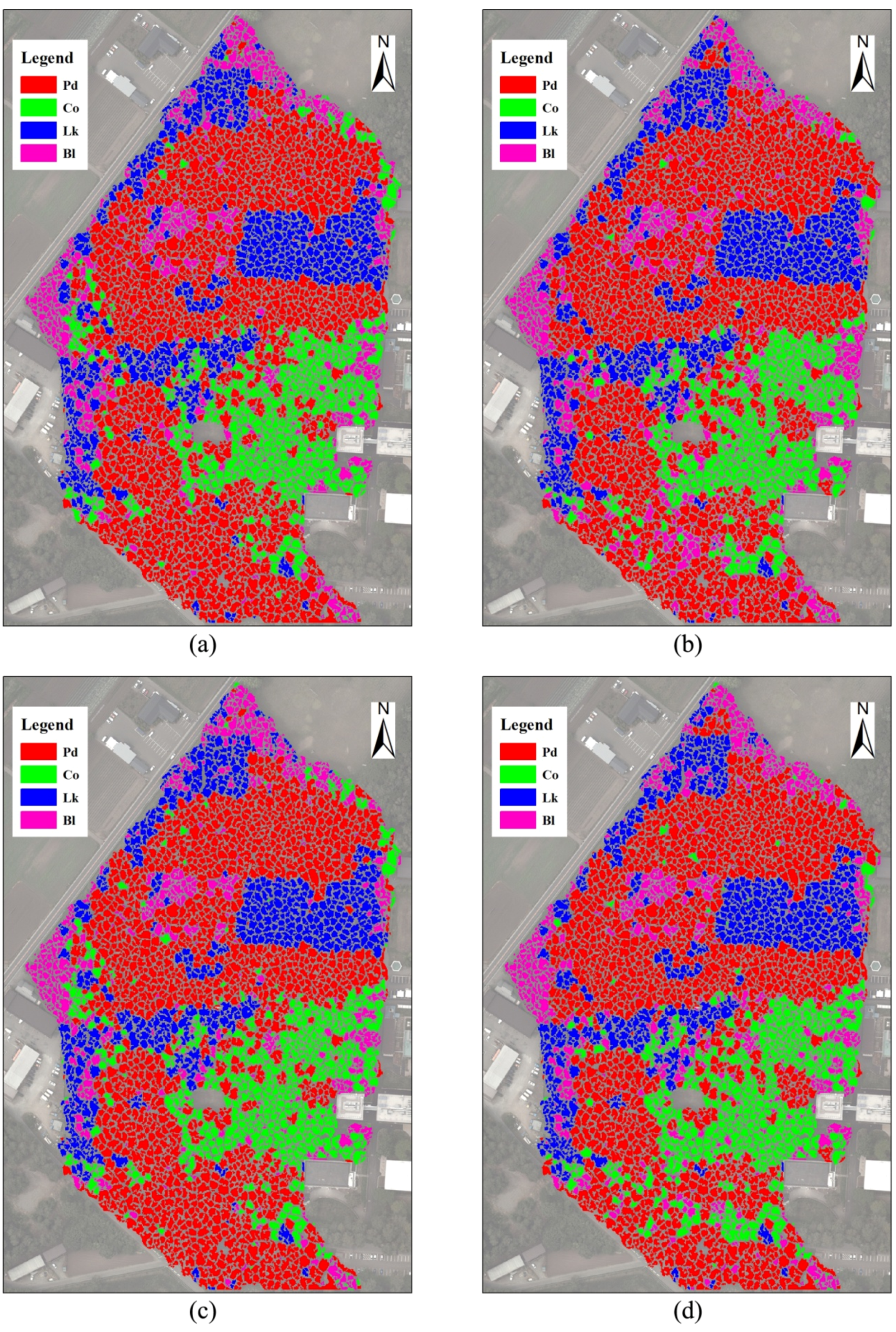
  • To determine whether the reflectance of forests on laser scanning and the average slope of tree crowns can contribute to forest classification; and
  • To compare the estimation capability of ALS data with that of optical bands for interpreting forest resources.

2. Materials and Methods
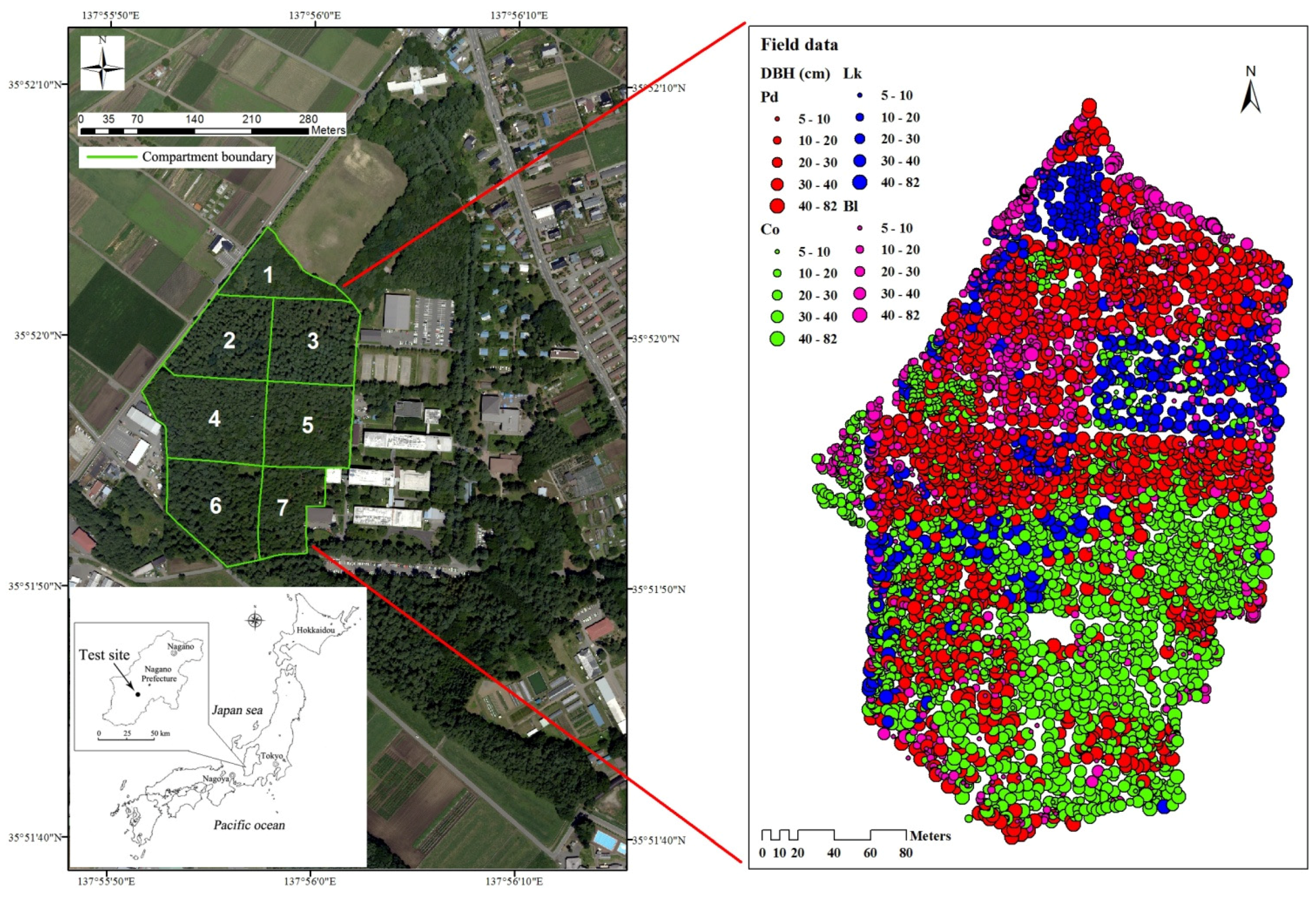
2.1. Study Area

The study area was the campus forest located in the Faculty of Agriculture at Shinshu University in Nagano Prefecture, central Honshu Island, Japan (Figure 1). The campus has an area of 52.7 ha, which includes approximately 15 ha of forest. The campus forest, with a total of 15 compartments, consists of high-density plantations with trees ranging from 30 to 90 years old and is a unique multipurpose educational training and research facility with wood production aimed at sustainable forest management [1]. Compartments 1–7 were selected as the test site in this study (Figure 1). The center of the study site is at 35°52′N, 137°56′E and has an altitude of 770 m above sea level. The area consists of smooth geographical features and flat land. The forests are mainly composed of conifer plantations in which the dominant tree species are Pinus densiflora (Pd), Chamaecyparis obtusa (Co), Larix kaempferi (Lk), and secondary broadleaved trees (Bl) (Figure 1).

2.2. Field Measurements and Geographic Information System (GIS) Data

In this study, we selected compartments 1–7 of the campus forest, with an area of approximately 7.3 ha, as the research object. All trees with a DBH larger than 5 cm in each compartment were surveyed, and the geographical position, species, DBH, and height were recorded. Each tree was tagged with a permanent label and noted as either live or dead, and the stems were mapped to the nearest 0.1 m and measured to the nearest 0.1 cm DBH. Tree heights were measured using Vertex IV (Haglöf, Långsele, Sweden), and tree locations were calculated using the geographic coordinates of the vertices of the plots, which were measured with a Global Positioning System (GPS) device (Garmin MAP 62SJ, Taiwan). All plot vertices were recorded when the GPS steadily displayed its highest accuracy, ±3 m, and the locations were post-processed with local base station and ALS data, resulting in an average error of approximately 0.5 m (within 2 pixels of the orthoimagery). The investigation was conducted from April 2005 to June 2007. Additionally, all trees in compartment 4 were surveyed again in June 2015 to determine whether the dominant tree species in the canopy layer changed. The results suggested no obvious changes in the canopy layer because no management activities, such as thinning or timber harvest, were conducted during this period. These field data were used to test the accuracy of the interpreted tree tops and to perform the supervised classifications of tree species (Figure 1). The conditions of the forests in the study area are summarized in Table 1. The DBH frequency distribution for all trees in the study area is shown in Figure 2.
In addition, compartment boundaries, forest roads, forest survey data, and geographical data, such as contour lines on the base map of the campus forest, were compiled for this study as a forest database using permanent marks located along the compartment edges. Moreover, all tree positions from the field survey were transferred and displayed using ArcGIS software (Esri, Redlands, CA, USA) (Figure 1) and then compared with the image analysis of the delineated crowns.

2.3. Airborne LiDAR Data
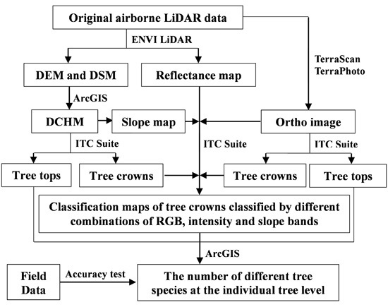
ALS data were acquired in June 2013 by a special public measurement project using a Leica ALS70-HP system (Leica Geosystems AG, Heerbrugg, Switzerland). The average flying altitude was 1800 m above ground level at a speed of 203 km/h, with a maximum scanning angle of ±15°, a beam divergence of 0.2 mrad and a pulse rate of 308 kHz. The wavelength of the laser scanner is 1064 nm. The sensor can record the first, second, third and last pulses reflected from the objects with the laser intensity. The lowest point density was ensured to be 4 points/m2. To obtain a high point density, the study area was overflown twice, with a large side overlap of 50%. Additionally, true color images with a resolution of 25 cm and three channels were obtained at the same time as the ALS data by the RCD30 sensor using the color mode. The original true-color images were ortho-rectified using the laser point data in TerraScan and TerraPhoto software.
The raw data were preprocessed by the measurement company, including producing the 3D point clouds, deleting noise points, and assessing the level of accuracy. The average vertical error was 0.031 m, with a root mean square error (RMSE) of 0.039 m, tested by 48 ground control points (GCPs). The maximum error between different courses was 0.09 m. The preprocessed original data with a las ver1.2 format and the orthophotos with red (R), green (G) and blue (B) bands were used in this study. The ALS data in the study area have a point density ranging from 13 to 30 points per m2. The original orthophotos with a resolution of 25 cm were rescaled to a resolution of 50 cm, which was most suitable for individual tree extraction [1,43,51].

2.4. Data Analyses

2.4.1. Interpretation of Airborne Laser Scanning (ALS) Data

The research flowchart in Figure 3 provides an overview of the methods. The original ALS data were first used to extract the digital elevation model (DEM) and digital surface model (DSM) with a resolution of 50 cm by the ENVI LiDAR software, and an intensity map of forest reflectance was simultaneously generated during processing. Second, the digital canopy height model (DCHM) was calculated by subtracting the DEM from the DSM using ArcGIS software. Then, the interpreted DCHM and forest reflectance intensity map with a 50 cm resolution were subjected to further analysis.
In laser scanning, the reflectance of objects can be calculated by the formula:
R = P r × S × e x p ( 2 μ H ) / ( P e × a )
where R is the reflectance of objects; Pr is the returned laser intensity; S is the beam spot area; μ is the attenuation coefficient caused by the atmosphere; H is the flying altitude; Pe is the emission intensity, and a is footprint area [52]. Prior to species classification, the reflectance image data were resampled as unsigned 8 bit integers.

2.4.2. Interpretation of Tree Tops Using the Individual Tree Crown (ITC) Approach

In this study, two types of tree tops were interpreted with the ITC approach in PCI Geomatica v9.1 software with the ITC Suite using the DCHM data generated in Section 2.4.1 and the green band of the orthophoto (Figure 3). The detailed steps of the interpretation are provided in previous studies [1,16,51,53]. First, preprocessing for the tree top interpretation was necessary to normalize the object bands based on their own ranges, which was performed twice to smooth using an averaging filter of 5 × 5 pixels (2.5 × 2.5 m) [1,51]. Second, a bitmap with a DCHM value of less than 5.0 m, which could be used to separate the forest caps, understory trees, and shrub and grass areas, was established for the non-forest mask by the THR (Thresholding Image to Bitmap, which can be used to create bitmaps with any threshold values) function. Additionally, the blue band with a value larger than 80 could be used to separate the man-made structures, such as monitoring towers built in the study area. Finally, the non-forested regions of the study site were extracted by the areas with a DCHM less than 5.0 m plus the pixels with a blue value larger than 80.
The ITC isolation image was produced using the valley-following algorithm [49]. Using the normalized DCHM and green bands and the non-forested mask, this method treats the spectral values as topography, with shaded and darker areas representing valleys and bright pixels delineating the tree crowns [1]. This method produces a bitmap of segments of valley and crown materials in forest areas. A rule-based system follows the boundary of each segment of crown material to create isolations, which are taken to represent tree crowns, whereas the pixel with the highest gray value at each tree crown is interpreted as the tree top by a local maximum filtering technique [33,51]. To better compare the results interpreted using different data, we only attempted to extract the tops of the canopy trees in the study area using a filter with a moving window of 5 × 5 pixels, which, in theory, may extract trees with a crown diameter of more than 2.5 m and has been proven effective in previous studies [16].
The interpreted accuracy of the tree tops can be calculated by the formula
φ = (1−|DI – Ds|/ Ds) × 100
where Φ is the interpreted accuracy (%), DI is the stem density of trees interpreted by the ITC method, and DS is the stem density of trees in the surveyed data. In this study, based on the DBH frequency distribution of all trees in the study area and the average DBH in each compartment (Figure 2, Table 1), the surveyed trees with a DBH larger than 25 cm were selected as the upper trees and used to test the accuracy of the interpreted tree tops in distinguishing species.

2.4.3. Supervised Classification and Counting for Different Tree Species

Different tree species have different three-dimensional crown shapes. We attempted to test whether the average slope of the tree crowns can contribute to the classification of the tree species in this study. Accordingly, a slope map was calculated using the DCHM data in ArcGIS software (Figure 3). Some authors suggested that the intensity of laser scanning with a wavelength of 1,064 nm could be used for tree species classification [40,52], but few studies of this type have been reported in Japan. Consequently, based on the field data and other information, including orthophotos and existing thematic maps, the extracted tree crowns in the study area were classified into four classes, Pinus densiflora (Pd), Chamaecyparis obtusa (Co), Larix kaempferi (Lk), and broadleaved trees (Bl), by using different combinations of the three bands of orthophoto with the intensity and slope maps: RGB; RGB and intensity (RGBI); RGB and slope (RGBS); and RGB, intensity and slope (RGBIS). All classifications were performed using the same training areas.
Moreover, several studies suggested that the object-based classification approach is better than the pixel-based approach in classifying mixed forests [16,54,55]. To overcome the “mixed pixels” problem of the pixel-based classification (i.e., some pixels within a tree crown may be classified into two or more different classes), an object-based supervised classifier (called crown-based classification) was designed for tree species classification in the ITC Suite [51] and used to generate thematic maps of the tree species in this study. This crown-based classification was completed by the ITCSC (Individual Tree Crown Supervised Classifier) function of the ITC Suite. The ITCSC classified the individual tree crowns (ITCs) of the images into different species using a maximum-likelihood (ML) decision rule [51]. The classification was based on comparing the signature of each ITC, one by one, with the ITC-based signatures of the various species. The species signatures (average spectral values in different bands) were produced by the ITCSSG (Individual Tree Crown Species Signatures Generation) program using the training crowns of different species.
Finally, when the tree top interpretation and supervised classification processes were completed, all tree tops were annotated with a species attribute from the species thematic maps delineated by the crown-based classification using an overlay by the extraction function in ArcGIS v10.0. The total number of trees of different species in each compartment was counted using the summarize function.

3. Results

In this study, two types of tree tops and tree crowns in the study area were delineated by the ITC approach using the green band of the orthophoto and the DCHM data, respectively. Then, the two types of tree crowns were classified into four classes, Pinus densiflora (Pd), Chamaecyparis obtusa (Co), Larix kaempferi (Lk), and broadleaved trees (Bl), by a crown-based classification approach using different combinations of the intensity and slope maps with the three bands of the orthophoto: RGB; RGBI; RGBS; and RGBIS. Consequently, eight thematic maps of tree species were generated in this study.

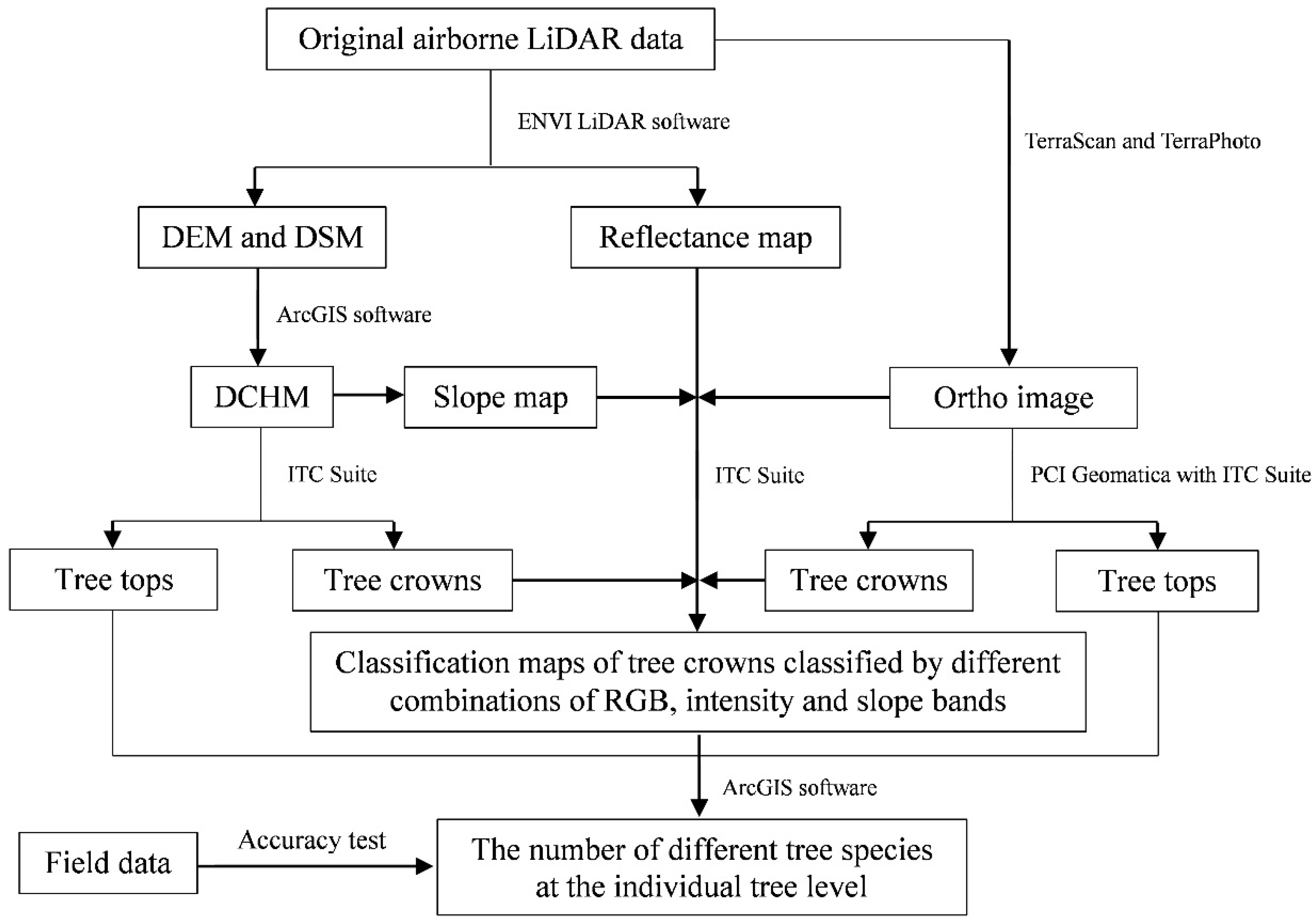
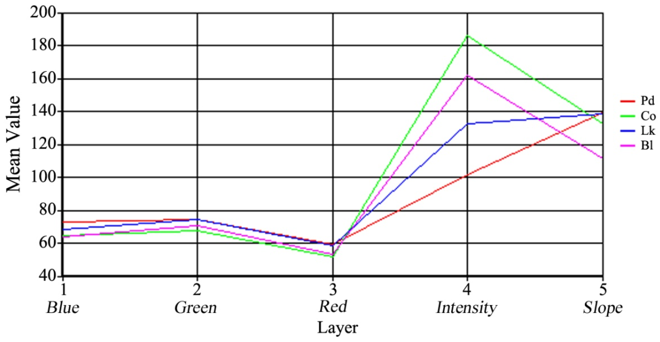
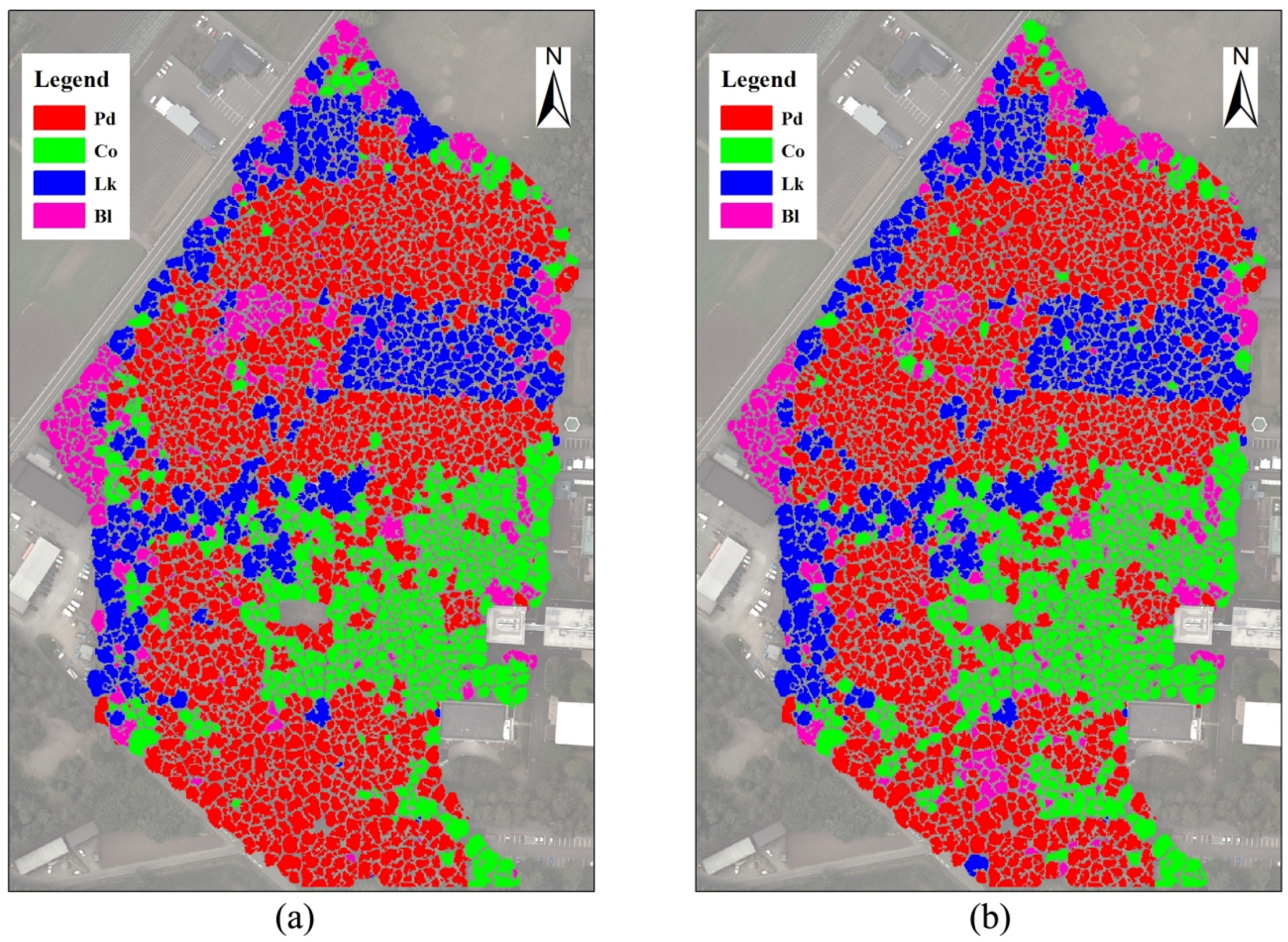
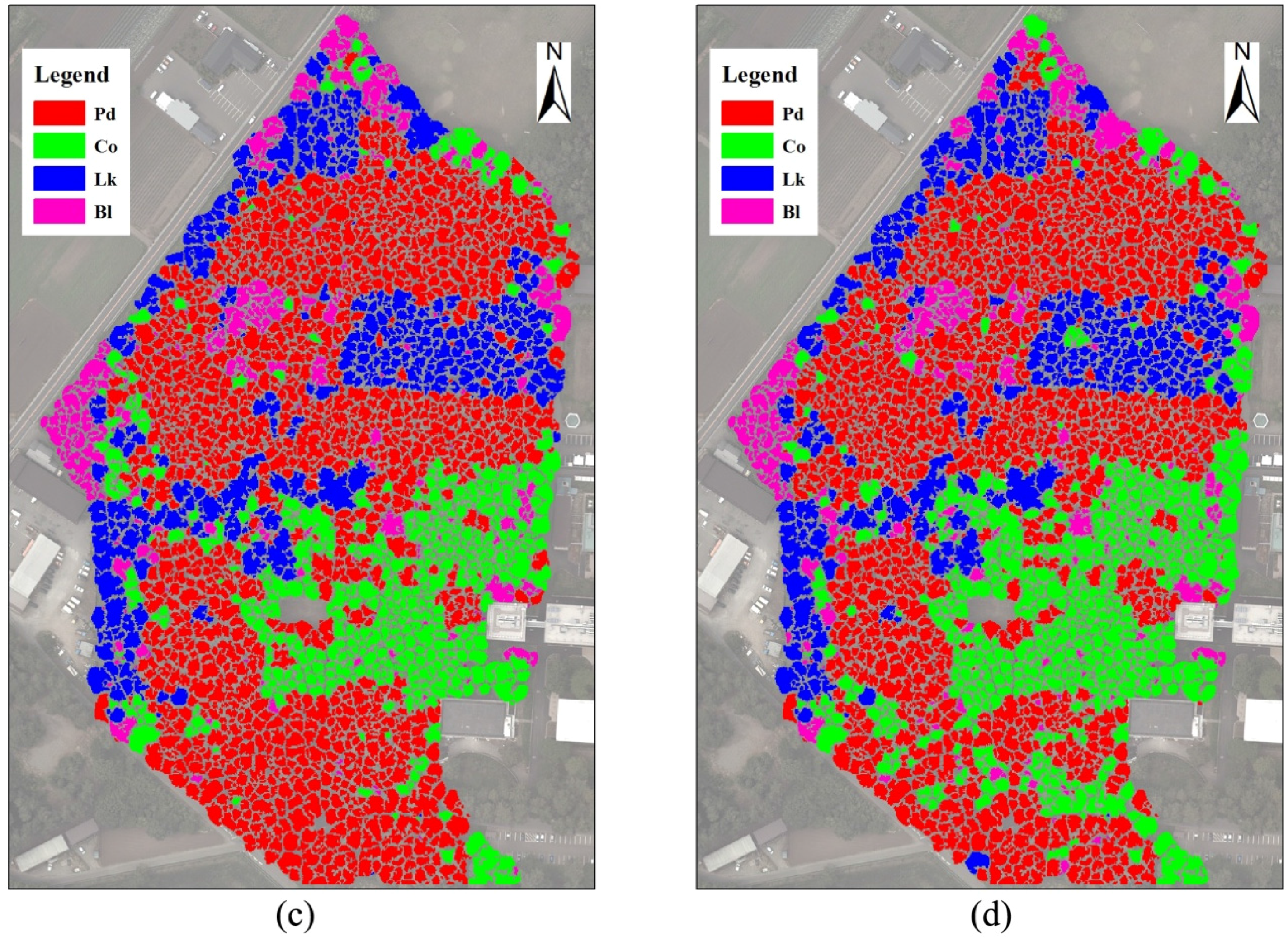
3.1. Object-Based Supervised Classification of Tree Species

3.1.1. Classification of the Tree Crowns Delineated Using the Green Band

Based on the field data and other information, four object-based supervised classifications were performed on the tree crowns detected using the green band of the orthophoto with RGB, RGBI, RGBS, and RGBIS. As a result, crown-based thematic maps of tree species were generated, as shown in Figure 4, by overlaying the true color image with a transparency of 50%.
In the classification process, 108 training areas were created for the four classes: Pd, 33; Co, 18; Lk, 27; and Bl, 30, and these training samples covered an area of 3513 m2 (4.9% of the total area of the test site). Using the mean digital number (DN, representing the reflectance of the objects to sunshine or laser and the average slope of the tree crowns) of the test pixels of each class, a straight-line map was used to compare the spectral characteristics of the different classes (Figure 5). In this research, the reflectance of the objects to sunshine or laser and the slope of the tree crowns were resampled to the data type of unsigned 8-bit integers. Band DNs for the spectral values of the orthophoto were highest for green and lowest for red for all classes. The mean DNs of the blue band were slightly lower than those of the green band. In terms of different species, only a slight difference was found in the three bands between the four classes. However, the figure shows that the reflectance band of the trees for the laser scanning was a good parameter for species classification in the study area. The tree crowns of Chamaecyparis obtusa and Pinus densiflora had the highest and lowest reflectance intensities, respectively. In addition, although the DNs of the average slope differed markedly between broadleaved and coniferous trees, only slight discrepancies were found in the conifers, such as Pinus densiflora and Larix kaempferi, which was disadvantageous for classifying them.
When the object-based classifications were completed, a total of 400 random sample trees were used for the accuracy assessment. Four hundred sample points were generated in the crown areas by the stratified random rule. Then, all sample trees were assigned their reference classes based on field data and other additional information, including high-resolution airborne multispectral images and existing thematic maps. Finally, an accuracy report was generated, as is displayed in Table 2. The results indicate that the overall accuracies of the classifications using RGBI, RGBS and RGBIS bands, with values of more than 76%, was higher than that using RGB bands, with a value of 70.8%. Within the tree species, conifers were typically classified with higher user accuracy than the broadleaved trees in the four classifications. With a range from 71.4% to 85.5%, the user accuracy of Pinus densiflora had a larger change between different classifications compared to other species. Additionally, the broadleaved trees were classified with an accuracy of less than 67%.

3.1.2. Classification of the Tree Crowns Delineated Using the Digital Canopy Height Model (DCHM)

Based on field data and other information, four object-based supervised classifications were performed on the tree crowns detected using the DCHM data with RGB, RGBI, RGBS, and RGBIS. Crown-based thematic maps of tree species were generated, as documented in Figure 6, by overlaying the true color image with a transparency of 50%.
When the object-based classifications were completed, a total of 400 random sample trees were used for the accuracy assessment. Four hundred sample points were generated in the crown areas by the stratified random rule. Then, all sample trees were assigned reference classes based on field data and other additional information, including high-resolution airborne multispectral images and existing thematic maps. Finally, an accuracy report was generated, as shown in Table 3. The confusion matrices indicate that the classification using RGB had a lower overall accuracy, with a value of 73.5%, than the other three classifications using the RGBI, RGBS and RGBIS bands. In terms of different tree species, although the three conifers were classified with a higher user accuracy than the broadleaved trees in the classification using RGB, the accuracy of the broadleaved species was nearly equal to or even higher than that of Chamaecyparis obtusa in the other three classifications. Additionally, Larix kaempferi had the highest classification accuracy among the four classes in the majority of the classifications. However, the accuracy of Chamaecyparis obtusa was less than 80% in the classifications.

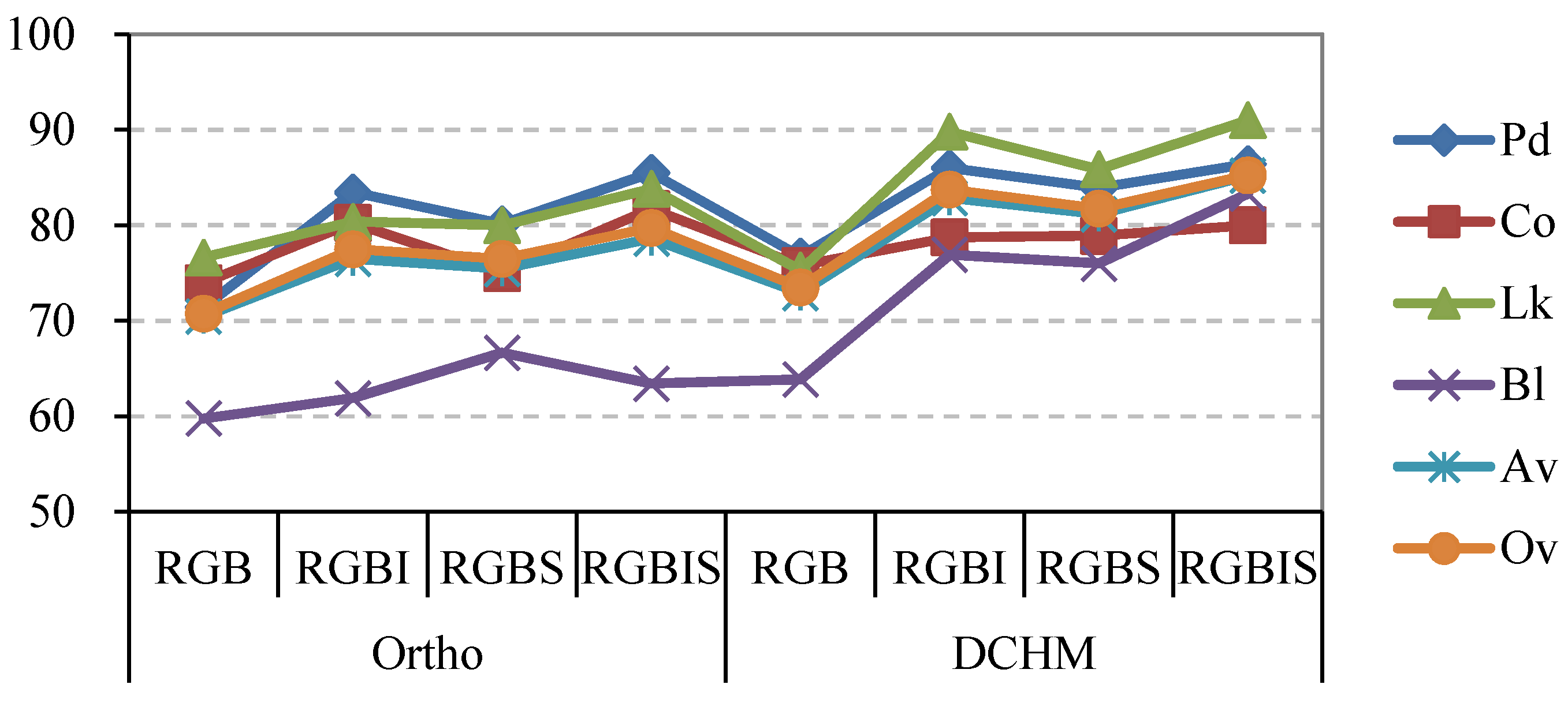
3.1.3. Comparison of Classifications of the Tree Crowns Detected Using Different Data

The user accuracies of different species for the classifications of tree crowns delineated and classified using different remotely sensed datasets are summarized in Figure 7. In terms of the overall and average accuracies, a discrepancy was found in the classifications of the tree crowns detected by the orthophoto and DCHM data, which had overall accuracies ranging from 70.8% to 79.8% and 73.5% to 85.8%, respectively. The average accuracy for each classification had a similar trend line to the overall accuracy. Regarding different tree species, the tree crowns of the four classes extracted using the DCHM data were classified with higher accuracy than those obtained by using the orthoimagery. For example, the crowns of Pinus densiflora delineated using the DCHM were classified with an improvement ranging from 0.9% to 5.3% when compared to the classifications of the tree crowns detected using the orthophoto. Additionally, the broadleaved trees were notably better classified by the tree crowns delineated using the DCHM data, with the highest average improvement of 12.1% among the four classes. By contrast, Chamaecyparis obtusa had the lowest average increment, with a value of 0.6%, because the accuracy of the tree crowns of Chamaecyparis obtusa detected using the DCHM data was slightly less than that using the orthoimage in the RGBI and RGBIS classifications. In terms of the combinations of different bands, the RGB classification had a lower accuracy than the other three classifications for most species. Although the tree crowns of Chamaecyparis obtusa delineated using the DCHM data were classified by the RGBIS with a relatively low accuracy of 80%, the broadleaved trees were classified by RGBIS bands with the highest accuracy among the eight classifications. The tree crowns obtained from the DCHM data had more stable classifications than those detected from the orthoimagery because the tree crowns were more accurately extracted using the DCHM data than using the orthophoto data.

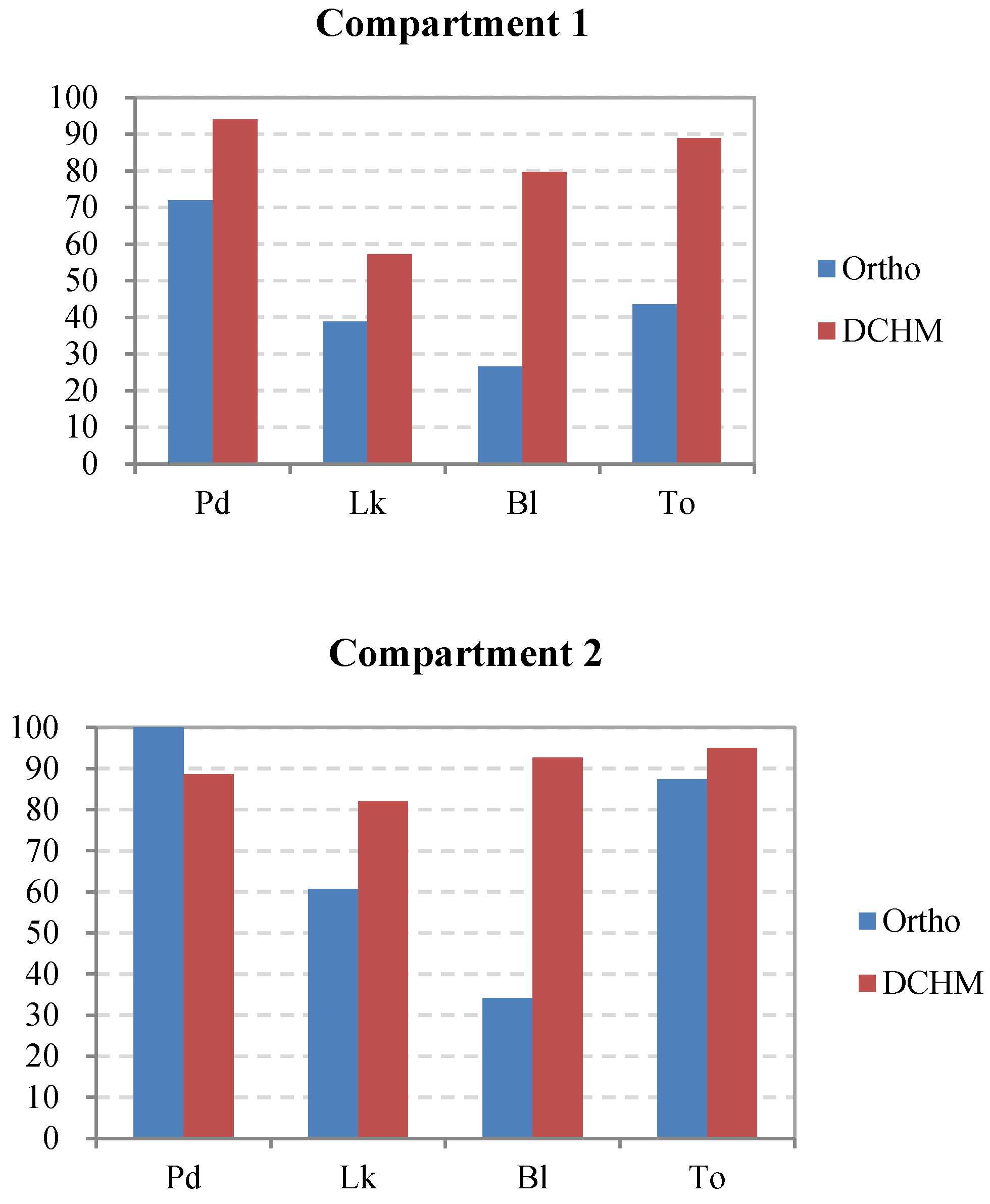
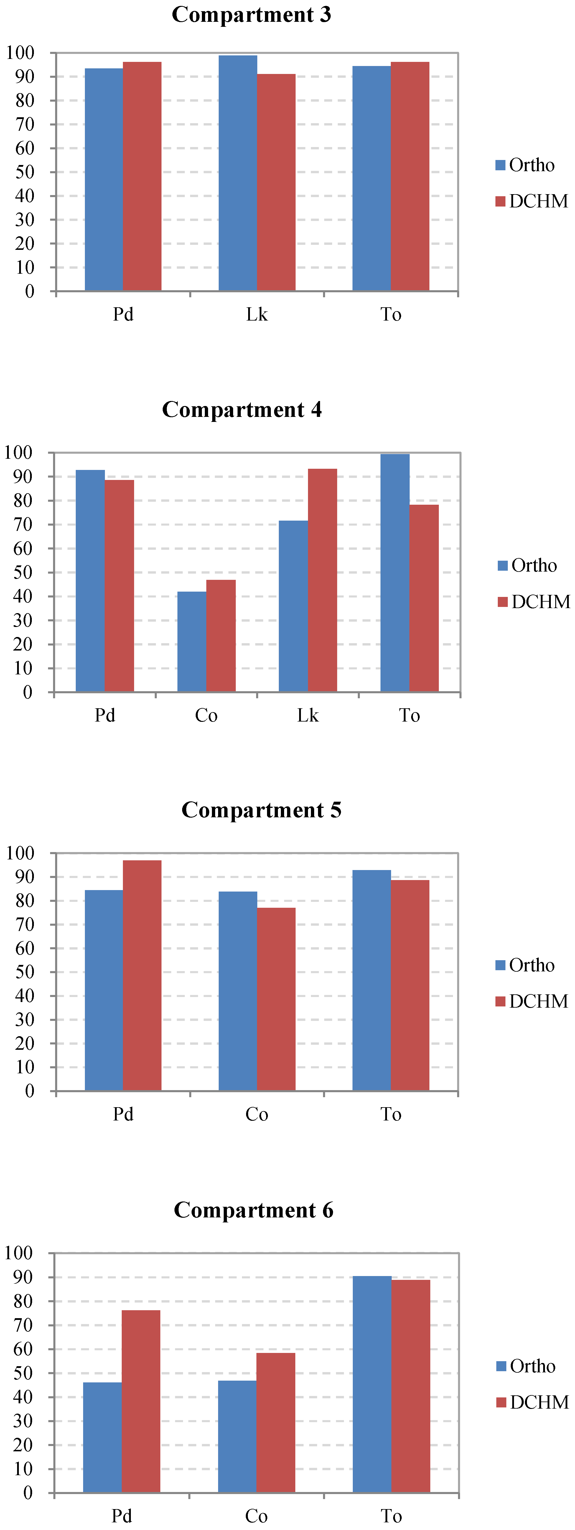
3.2. Counting Trees of Different Species in the Study Area

In this study, using an overlay from the extraction function in ArcGIS v10.0, all tree tops extracted by the ITC method were annotated with species attributes from the two thematic maps of the tree crowns generated by the orthophoto and DCHM data and classified by the crown-based approach using the RGBIS combination, which had better results than the other three combinations of RGB, RGBI and RGBS, as proven in the accuracy assessments. The total numbers of trees of different species in each compartment and in the entire study area were counted using the summarize function (Table 4). The number of overstory trees with a DBH larger than 25 cm recorded in the field data is also listed in Table 4. The count indicates that the density of the forest in compartment 1 is mainly dominated by Pinus densiflora, Larix kaempferi and broadleaved trees. However, Pinus densiflora is the most dominant species in compartment 2. The forest in compartment 3 is dominated by Pinus densiflora and Larix kaempferi. Compartment 4, which has the highest stem density and the most complex spatial structure among the seven compartments, is mainly dominated by Pinus densiflora, Chamaecyparis obtusa and Larix kaempferi, and the forests in compartments 5–7 are dominated by Pinus densiflora and Chamaecyparis obtusa. The interpreted results of the most dominant species in the different compartments are in accordance with the forest inventory data, except for broadleaved trees. The number of broadleaved trees extracted from the orthoimages in many compartments was evidently more than that counted from the field data. Moreover, many Chamaecyparis obtusa trees failed to be delineated in compartments 4 and 6.
In addition, the interpreted accuracies of the dominant tree species were calculated using Equation (2). The results are shown in Figure 8. The dominant tree species in compartments 3 and 5, which have relatively simple spatial structures compared to the other compartments, were detected with a high level of accuracy. Conversely, some dominant trees, such as Chamaecyparis obtusa, in compartments 4 and 6, where the forests had a high stem density and a complex structure of multiple layers, were delineated with a relatively low accuracy of less than 60% because the probability of overlap between crowns increases with the stem density. However, in compartment 7, although the total number of the tree tops was extracted with an accuracy of 100% by using the green band of the orthophoto data, Pinus densiflora was not interpreted well because the forest had the highest mixing degree between the dominant trees, which was disadvantageous for classification. Additionally, as one of the dominant species in compartments 1 and 2, the broadleaved trees were extracted with an evidently lower accuracy using the orthoimage instead of the DCHM data because the broadleaved trees had a dispersive crown, which easily led to one tree crown being detected as several crowns. Consequently, the excessive number of broadleaved trees delineated from the orthoimagery led to the extremely low interpreted accuracy at −28.8% in the entire study area (Figure 8). Overall, the interpretation of the most dominant species using the DCHM data was better than that using the orthophoto data.

3.3. Accuracy of Position Matching of Interpreted Trees with Surveyed Trees

In this study, matching analyses were used to estimate the errors of omission (the trees that were not detected by remotely sensed data) and commission (the treetop candidates that could not be linked to field trees). Three thematic maps with a resolution of 5 m (the average distance between tree tops) were established by nearest neighborhood interpolation. One was created using the field data (FD), and the other two maps used the two tree top datasets annotated with species attributes from the two species maps of the tree crowns that were generated by the orthophoto (OP) and DCHM data (DD), respectively. Then, two matching analyses were conducted between FD and OP and between FD and DD, and the error matrices for the two matchings are listed in Table 5. The results indicate that, between OP and FD, the matching of the four classes had a commission accuracy ranging from 58.3% to 84.1% while its omission accuracy ranged from 69.8% to 81.5%. A remarkable matching discrepancy was found between the tree positions detected by the orthophoto and DCHM data and those recorded in the field, which had overall matching accuracies of 75.6% and 85.7%, respectively. In terms of the different tree species, the tree positions of the four classes extracted using the DCHM data were matched to the field data with greater accuracy than those obtained using the orthoimagery. The commission accuracy of the matching between DD and FD improved from 6.6% to 15.3% when compared to the matching between OP and FD, and the omission accuracy was improved from 4.7% to 13.8% by matching DD and FD. The findings from this study indicate that the positions of the trees were more accurately delineated using the DCHM data than the orthophoto data.

4. Discussion

Obtaining spatially detailed forest information at the tree level over large areas is critical for sustainable forest management [4,16]. This task has been enabled by the advent of airborne digital sensors and the launch of commercial satellites that can obtain multispectral imageries with a high resolution of 1 m or less in panchromatic mode [1,2,9,10,11,12,13,14,15]. However, it is difficult to detect the three-dimensional attributes of forests, such as tree height and DBH, using only optical data [16,41]. Accordingly, the LiDAR technology has received increasing attention from researchers in the forest measurement field [17,18,20,21,22,23,24,25,26,27,28,29,30,31,32,33,34,35,36,37,38,39,40]. However, it is difficult to classify the tree crowns delineated from the mixed forests based purely on the point cloud data [39,40]. This study attempted to acquire forest resource information at the individual tree level by combining the LiDAR point cloud with the true color images obtained at the same time as the laser scanning data.
For a large forest composed of uneven-aged stands with different tree crown sizes, the homogeneity function of the ITC Suite can be used to separate young tree areas from mature forests [1,24]; the tops of small and large-sized trees can then be interpreted using filters with different moving window sizes on small and large tree areas, respectively [16]. In this study, however, because of the high canopy density, it is nearly impossible to interpret the trees in the understory using the DCHM and true color data. Additionally, the forests in the study area are derived from the man-made stands, and thus, most trees in the upper layer had a similar crown size. Consequently, a filter with a fixed moving window of 5 × 5 pixels was used on the tree tops in the present study, which, in theory, should extract trees with a crown diameter of greater than 2.5 m [1,16,49,51]. Although some authors indicated that it is possible to delineate the understory trees in some forests with a moderate canopy density using the ALS data collected in different seasons [52], the point density reflected from the understory trees in our study was sufficiently low that small trees were unable to be extracted using only these points because the forests had a high canopy density, and the data were obtained in the summer, in which most trees had the highest leaf area index (LAI). Therefore, it is essential to interpret the forests by combining the data acquired in a leaf-on situation with those acquired in a leaf-off situation in future studies. In addition, the advent of terrestrial laser scanning (TLS), which has been successfully used to measure the tree size and volume in several boreal forests [39,56,57,58,59,60,61], provides a new approach to delineating small trees in the under layer. However, the usefulness of this sensor for various types of vegetation remains to be verified, especially for the dense forests in Japan.
Because orthophoto data were always obtained simultaneously with the ALS data in the measurements, this study aimed to test the possibility of classifying forests by combining the optical bands and the features derived from ALS data. As a comparison, two types of tree crown were delineated by the ITC approach using the DCHM data and the green band of the orthophoto, respectively. When the tree crown delineations were completed, four object-based supervised classifications were conducted for each type of tree crown using combinations of the different features, including the reflectance of the optical bands and laser and the slope of the tree crowns. The classification accuracy was improved in this study for all tree species with the use of the forest reflectance and the slope of the tree crowns, which led to increased separability of the classes (Figure 5). In the classifications of the tree crowns delineated by the green band and DCHM data, the improvements of the overall accuracy ranged from 5.7% for the RGBS to 9.0% for the RGBIS and from 8.3% for the RGBS to 11.8% for the RGBIS when compared to the RGB, respectively (Table 2 and Table 3). This higher level of accuracy was obtained because the added features of laser intensity and slope contribute to the classifications (Figure 5). The results suggest that the reflectance of the trees in the laser scanning may be a valuable source of information for the tree species classification of Pinus densiflora, Chamaecyparis obtusa and Larix kaempferi, which are the main tree species in Japan. However, the usefulness of the added features in the classification should be further tested by application to other forests during different seasons. In addition, we attempted to classify the forests using only the variables derived from the LiDAR data: crown diameter, crown height, crown area and crown volume. Several combinations were used for the classification without the orthophoto spectral bands, but the results were poor, with an overall accuracy ranging from 34% to 50%. Therefore, these classifications were not included in this study. The contribution of different features derived from LiDAR data and multispectral image to species classification will be further discussed in the next study on the comparison of individual tree delineations using different detection approaches.
Additionally, some authors classified the boreal forests using only the point cloud data obtained from airborne laser scanning. For example, Yu et al. (2014) classified pine, spruce and birch in southern Finland using 15 features extracted from the ALS data, resulting in an overall accuracy of 73.4% [40]. In Heinzel and Koch, an accuracy of 78% was achieved for the classification of four species (pine, spruce, oak and beech) [62]. In Hollaus et al., three tree species (red beech, larch and spruce) were classified with an overall accuracy at 75% [63]. Most of the previous studies that classified forests based solely the features extracted from ALS data reported overall accuracies ranging from 57% to 83% [40,62,63,64,65,66,67,68,69]. All of these studies have demonstrated the usefulness of the ALS-derived features in tree species classification. Consequently, further investigations are needed to study the impact of combining optical bands with more ALS-based features in species classification.
Classification accuracy is not balanced between the tree species. Pinus densiflora and Larix kaempferi were classified with a higher accuracy than the other species. However, the user accuracy for broadleaved trees is relatively poor (i.e., less than 67%) using the tree crowns detected from the orthophoto data in the classifications. The reason for this result is likely related to the difficulties in the accurate delineation of broadleaved tree crowns because of the more complex crown shape and structure. Due to the dispersive crown shape, the ITC algorithm tends to split large deciduous trees into multiple crown parts when using the optical image with high resolution, which results in one segment for each part. However, the classified accuracy of broadleaved trees is considerably higher, with the best result of 83.3%, when using the tree crowns delineated from the DCHM data in the classifications (Figure 7). Additionally, errors in the classification can be attributed to the lack of near-infrared (NIR) information. Numerous studies suggested that NIR bands improved the accuracy of tree species classification in different study areas [4,5,16]. In Katoh et al. [1], the broadleaved trees were classified with an accuracy of 97% by the ITC approach using airborne multispectral images with a resolution of 50 cm and four bands of blue, green, red and NIR in the same area as this study. Therefore, the contribution of NIR information, which can be obtained in the ALS measurements using the colorIR mode, to the detection of broadleaved trees requires further study.
In terms of the distinguishing species for individual tree delineation, the trees were better extracted in the compartments with a relatively simple stand structure compared to other compartments. For example, Chamaecyparis obtusa was delineated with an accuracy of less than 60% in compartments 4 and 6 because the forests had a high stem density and a complex structure of multiple layers, which increases the probability of overlap between crowns. Although the total number of tree tops was extracted with a high accuracy in compartment 7, Pinus densiflora was interpreted at less than 30% using the tree crowns detected from the green band of the orthophoto data because the forest had the highest degree of mixing, which was disadvantageous for classification. Additionally, the broadleaved trees were detected with low accuracy using the orthoimage. This result can be attributed to the dispersive crowns of broadleaved trees and the overly high resolution of the orthophotos, with a value of 25 cm in the original data, which easily led to one tree crown being split into several crowns. The above reasoning can also explain the better delineation of the most dominant species using the DCHM data compared to using the orthophoto data in the study area (Figure 8). Moreover, the DBHs of individual trees can be accurately measured by regression models using DBH as the dependent variable and tree height as the independent variable and combining the location information of the extracted tree tops. Consequently, the present study recommends delineating tree crowns using DCHM data instead of optical data. In addition, several authors delineated individual trees in boreal forests with high accuracy using ALS data by the individual tree detection (ITD) algorithm [34,37,40,70,71,72]. Although our study achieved comparable tree detection results, further research is required to study the influence of different approaches on tree delineation [73]. Further improvements are possible for individual tree detection using 3D segmentation techniques that utilize more spatial information provided by the ALS data [40].
In this study, field data from April 2005 to June 2007 were used to test the interpreted accuracy, whereas the ALS data were obtained in June 2013. Although a slight discrepancy was found in the accuracies calculated using the inventory data surveyed in 2007 and 2015 for compartments 4 and 6, the detection results for other compartments must be tested using recent field data that will be collected in 2016. Additionally, the surveyed trees with a DBH larger than 25 cm were selected as the upper trees of the study area and used to test the accuracy of the interpreted tree top distinguishing species. In fact, a notable difference in the stand structure was found between some compartments. Accordingly, the selection method of upper trees for different forests should be explored in future studies. Each compartment was selected as the unit of the interpreted accuracy calculation, which likely resulted in the improvement of the tree detection results of some species because the confusion of misclassified species may offset their number in the delineation with each other.

5. Conclusions

Accurate tree delineation and species classification are critical for the interpretation of the individual-based volume and biomass of forests. In this study, we assessed the utility of ALS data for individual tree detection and species classification in a mixed forest with a high canopy density in Japan. For comparison, the two types of tree tops and tree crowns in the study area were delineated by the ITC approach using the green band of the orthophoto and the DCHM data derived from the airborne laser scanning. Then, both types of tree crown were classified into four classes, Pinus densiflora (Pd), Chamaecyparis obtusa (Co), Larix kaempferi (Lk), and broadleaved trees (Bl), by an object-based classification approach using the different combinations of the laser intensity and slope maps with the three bands of the orthophoto: RGB, RGBI, RGBS, and RGBIS. The results of our study suggest that the combination of RGBIS yielded a higher classification accuracy than other combinations. The added features of laser intensity and slope derived from ALS data contributed to the classifications. The reflectance of the trees on the laser scanning may be a valuable source of information for the tree species classification of Pinus densiflora, Chamaecyparis obtusa and Larix kaempferi, which are the main tree species in Japan. However, its usefulness must be verified in future studies by application in other forests. The exploration of other ALS-based features, such as the mean height and diameter of tree crowns, is recommended for future research related to tree species classification. In addition, the findings from this study demonstrate the advantage using DCHM data instead of optical data in delineating tree crowns. Further improvements can be achieved for individual tree detection using 3D segmentation techniques that can utilize more spatial information provided by the ALS data. Consequently, additional research is required for detecting individual trees in the study area using other delineation algorithms, such as the ITD approach.

Acknowledgments

This study was supported by a Grant-in-Aid for Scientific Research from the Japan Society for the Promotion of Science (No. 24380077). We gratefully acknowledge a number of students of Shinshu University for their support in the field and plot survey. We would like to thank the members of the Forest Measurement and Planning Laboratory, Shinshu University, for their advice and assistance with this study. Moreover, we wish to express our heartfelt thanks to François A. Gougeon for providing ITC Suite, an ideal procedure for forest inventories using remotely sensed images. Finally, we wish to acknowledge the helpful comments from the anonymous reviewers and editors.

Author Contributions

Songqiu Deng designed the experiment. Masato Katoh coordinated the research projects and provided technical support and conceptual advice. Songqiu Deng and Masato Katoh performed the experiments, collected the data and completed the manuscript. All of the authors helped in the preparation and revision of the manuscript.

Conflicts of Interest

The authors declare no conflict of interest.

References

  1. Katoh, M.; Gougeon, F.A.; Leckie, D.G. Application of high-resolution airborne data using individual tree crown in Japanese conifer plantations. J. For. Res. 2009, 14, 10–19. [Google Scholar] [CrossRef]
  2. Katoh, M.; Gougeon, F.A. Improving the precision of tree counting by combining tree detection with crown delineation and classification on homogeneity guided smoothed high resolution (50 cm) multispectral airborne digital data. Remote Sens. 2012, 4, 1411–1424. [Google Scholar] [CrossRef]
  3. Zolkos, S.G.; Goetz, S.J.; Dubayah, R. A meta-analysis of terrestrial aboveground biomass estimation using LiDAR remote sensing. Remote Sens. Environ. 2013, 128, 289–298. [Google Scholar] [CrossRef]
  4. Immitzer, M.; Atzberger, C.; Koukal, T. Tree species classification with random forest using very high spatial resolution 8-band WorldView-2 satellite data. Remote Sens. 2012, 4, 2661–2693. [Google Scholar] [CrossRef]
  5. Straub, C.; Weinacker, H.; Koch, B. A comparison of different methods for forest resource estimation using information from airborne laser scanning and CIR orthophotos. Eur. J. For. Res. 2010, 129, 1069–1080. [Google Scholar] [CrossRef]
  6. Nagendra, H. Using remote sensing to assess biodiversity. Int. J. Remote Sens. 2001, 22, 2377–2400. [Google Scholar] [CrossRef]
  7. Clark, M.L.; Roberts, D.A.; Clark, D.B. Hyperspectral discrimination of tropical rain forest tree species at leaf to crown scales. Remote Sens. Environ. 2005, 96, 375–398. [Google Scholar] [CrossRef]
  8. Larsen, M. Single tree species classification with a hypothetical multi-spectral satellite. Remote Sens. Environ. 2007, 110, 523–532. [Google Scholar] [CrossRef]
  9. Hill, D.A.; Leckie, D.G. Forest regeneration: Individual tree crown detection techniques for density and stocking assessments. In Proceedings of the International Forum on Automated Interpretation of High Spatial Resolution Digital Imagery for Forestry, Victoria, BC, Canada, 10–12 February 1998; pp. 169–177.
  10. Leckie, D.G.; Gillis, M.D. A crown-following approach to the automatic delineation of individual tree crowns in high spatial resolution aerial images. In Proceedings of the International Forum on Airborne Multispectral Scanning for Forestry and Mapping, Chalk River, ON, Canada, 13–16 April 1993; pp. 86–93.
  11. Pollock, R. A Model-based approach to automatically locating individual tree crowns in high-resolution images of forest canopies. In Proceedings of the First International Airborne Remote Sensing Conference and Exhibition, Strasbourg, France, 12–15 September 1994; pp. 11–15.
  12. Wang, L.; Gong, P.; Biging, G.S. Individual tree-crown delineation and treetop detection in high-spatial resolution aerial imagery. Photogramm. Eng. Remote Sens. 2004, 70, 351–357. [Google Scholar] [CrossRef]
  13. Erikson, M. Segmentation of individual tree crowns in color aerial photographs using region growing supported by fuzzy rules. Can. J. For. Res. 2003, 33, 1557–1563. [Google Scholar] [CrossRef]
  14. Katoh, M. Comparison of high resolution IKONOS imageries to interpret individual trees. J. Jpn. For. Soc. 2002, 84, 221–230. [Google Scholar]
  15. Gougeon, F.A.; Leckie, D.G. The individual tree crown approach applied to IKONOS images of a coniferous plantation area. Photogramm. Eng. Remote Sens. 2006, 72, 1287–1297. [Google Scholar] [CrossRef]
  16. Deng, S.; Katoh, M.; Guan, Q.; Yin, N.; Li, M. Interpretation of forest resources at the individual tree level at Purple Mountain, Nanjing City, China, using WorldView-2 imagery by combining GPS, RS and GIS technologies. Remote Sens. 2014, 6, 87–110. [Google Scholar] [CrossRef]
  17. Lefsky, M.A.; Cohen, W.B.; Acker, S.A.; Parker, G.G.; Spies, T.A.; Harding, D. LiDAR remote sensing of the canopy structure and biophysical properties of Douglas-fir western hemlock forests. Remote Sens. Environ. 1999, 70, 339–361. [Google Scholar] [CrossRef]
  18. Popescu, S.C.; Wynne, R.H.; Scrivani, J.A. Fusion of small-footprint LiDAR and multi-spectral data to estimate plot-level volume and biomass in deciduous and pine forests in Virginia, USA. For. Sci. 2004, 50, 551–565. [Google Scholar]
  19. Deng, S.; Katoh, M.; Guan, Q.; Yin, N.; Li, M. Estimating forest aboveground biomass by combining ALOS PALSAR and WorldView-2 data: A case study at Purple Mountain National Park, Nanjing, China. Remote Sens. 2014, 6, 7878–7910. [Google Scholar] [CrossRef]
  20. Næsset, E.; Gobakken, T. Estimation of above- and below-ground biomass across regions of the boreal forest zone using airborne laser. Remote Sens. Environ. 2008, 112, 3079–3090. [Google Scholar] [CrossRef]
  21. Zhao, K.G.; Popescu, S.; Nelson, R. LiDAR remote sensing of forest biomass: A scale in variant estimation approach using airborne lasers. Remote Sens. Environ. 2009, 113, 182–196. [Google Scholar] [CrossRef]
  22. Sun, G.; Ranson, K.J. Modeling LiDAR returns from forest canopies. IEEE Trans. Geosci. Remote Sens. 2000, 38, 2617–2626. [Google Scholar]
  23. Patenaude, G.; Hill, R.; Milne, R.; Gaveau, D.; Briggs, B.; Dawson, T. Quantifying forest above ground carbon content using LiDAR remote sensing. Remote Sens. Environ. 2004, 93, 368–380. [Google Scholar] [CrossRef]
  24. Lee, A.; Lucas, R.M. A LiDAR derived canopy density model for tree stem and crown mapping in Australian woodlands. Remote Sens. Environ. 2007, 111, 493–518. [Google Scholar] [CrossRef]
  25. Mitchard, E.T.A.; Saatchi, S.S.; White, L.J.T.; Abernethy, K.A.; Jeffery, K.J.; Lewis, S.L.; Collins, M.; Lefsky, M.A.; Leal, M.E.; Woodhouse, I.H.; et al. Mapping tropical forest biomass with radar and spaceborne LiDAR in Lopé National Park, Gabon: Overcoming problems of high biomass and persistent cloud. Biogeosciences 2012, 9, 179–191. [Google Scholar] [CrossRef]
  26. Montesano, P.M.; Cook, B.D.; Sun, G.; Simard, M.; Nelson, R.F.; Ranson, K.J.; Zhang, Z.; Luthcke, S. Achieving accuracy requirements for forest biomass mapping: A spaceborne data fusion method for estimating forest biomass and LiDAR sampling error. Remote Sens. Environ. 2013, 130, 153–170. [Google Scholar] [CrossRef]
  27. Næsset, E. Estimating timber volume of forest stands using airborne laser scanner data. Remote Sens. Environ. 1997, 61, 246–253. [Google Scholar] [CrossRef]
  28. Breidenbach, J.; Koch, B.; Kandler, G. Quantifying the influence of slope, aspect, crown shape and stem density on the estimation of tree height at plot level using LiDAR and InSAR data. Int. J. Remote Sens. 2008, 29, 1511–1536. [Google Scholar] [CrossRef]
  29. Tsuzuki, H.; Nelson, R.; Sweda, T. Estimating timber stock of Ehime Prefecture, Japan using airborne laser profiling. J. For. Plann. 2008, 13, 259–265. [Google Scholar]
  30. Kodani, E.; Awaya, Y. Estimating stand parameters in manmade coniferous forest stands using low-density LiDAR. J. Jpn. Soc. Photogram. Remote Sens. 2013, 52, 44–55. [Google Scholar] [CrossRef]
  31. Hayashi, M.; Yamagata, Y.; Borjigin, H.; Bagan, H.; Suzuki, R.; Saigusa, N. Forest biomass mapping with airborne LiDAR in Yokohama City. J. Jpn. Soc. Photogram. Remote Sens. 2013, 52, 306–315. [Google Scholar] [CrossRef]
  32. Takejima, K. The development of stand volume estimation model using airborne LiDAR for Hinoki (Chamaecyparis obtusa) and Sugi (Cryptomeria japonica). J. Jpn. Soc. Photogram. Remote Sens. 2015, 54, 178–188. [Google Scholar]
  33. Wulder, M.; Niemann, K.O.; Goodenough, D.G. Local maximum filtering for the extraction of tree locations and basal area for high spatial resolution imagery. Remote Sens. Environ. 2000, 73, 103–114. [Google Scholar] [CrossRef]
  34. Hyyppä, J.; Kelle, O.; Lehikoinen, M.; Inkinen, M. A segmentation-based method to retrieve stem volume estimates from 3-D tree height models produced by laser scanners. IEEE Trans. Geosci. Remote Sens. 2001, 39, 969–975. [Google Scholar] [CrossRef]
  35. Takahashi, T.; Yamamoto, K.; Senda, Y.; Tsuzuku, M. Predicting individual stem volumes of sugi (Cryptomeria japonica D. Don) plantations in mountainous areas using small-footprint airborne LiDAR. J. For. Res. 2005, 10, 305–312. [Google Scholar] [CrossRef]
  36. Chen, Q.; Gong, P.; Baldocchi, D.; Tian, Y. Estimating basal area and stem volume for individual trees from LiDAR data. Photogramm. Eng. Remote Sens. 2007, 73, 1355–1365. [Google Scholar] [CrossRef]
  37. Kankare, V.; Räty, M.; Yu, X.; Holopainen, M.; Vastaranta, M.; Kantola, T.; Hyyppä, J.; Hyyppä, H.; Alho, P.; Viitala, R. Single tree biomass modelling using airborne laser scanning. ISPRS J. Photogram. Remote Sens. 2013, 85, 66–73. [Google Scholar] [CrossRef]
  38. Hauglin, M.; Gobakken, T.; Astrup, R.; Ene, L.; Næsset, E. Estimating single-tree crown biomass of Norway spruce by airborne laser scanning: A comparison of methods with and without the use of terrestrial laser scanning to obtain the ground reference data. Forests 2014, 5, 384–403. [Google Scholar] [CrossRef]
  39. Kankare, V.; Liang, X.; Vastaranta, M.; Yu, X.; Holopainen, M.; Hyyppä, J. Diameter distribution estimation with laser scanning based multisource single tree inventory. ISPRS J. Photogram. Remote Sens. 2015, 108, 161–171. [Google Scholar] [CrossRef]
  40. Yu, X.; Litkey, P.; Hyyppä, J.; Holopainen, M.; Vastaranta, M. Assessment of low density full-waveform airborne laser scanning for individual tree detection and tree species classification. Forests 2014, 5, 1011–1031. [Google Scholar] [CrossRef]
  41. Deng, S.; Katoh, M. Change of spatial structure characteristics of the forest in Oshiba Forest Park in 10 years. J. For. Plann. 2011, 17, 9–19. [Google Scholar]
  42. Leckie, D.G.; Gougeon, F.A.; Walsworth, N.; Paradine, D. Stand delineation and composition estimation using semi-automated individual tree crown analysis. Remote Sens. Environ. 2003, 85, 355–369. [Google Scholar] [CrossRef]
  43. Leckie, D.G.; Gougeon, F.A.; Tinis, S.; Nelson, T.; Burnett, C.N.; Paradine, D. Automated tree recognition in old growth conifer stands with high resolution digital imagery. Remote Sens. Environ. 2005, 94, 311–326. [Google Scholar] [CrossRef]
  44. Ke, Y.; Zhang, W.; Quackenbush, L.J. Active contour and hill climbing for tree crown detection and delineation. Photogramm. Eng. Remote Sens. 2010, 76, 1169–1181. [Google Scholar] [CrossRef]
  45. Katoh, M. The identification of large size trees. In Forest Remote Sensing: Applications from Introduction, 3rd ed.; Japan Forestry Investigation Committee: Tokyo, Japan, 2010; pp. 308–309. [Google Scholar]
  46. Ke, Y.; Quackenbush, L.J. A comparison of three methods for automatic tree crown detection and delineation methods from high spatial resolution imagery. Int. J. Remote Sens. 2011, 32, 3625–3647. [Google Scholar] [CrossRef]
  47. Culvenor, D.S. Extracting individual tree information. In Remote Sensing of Forest Environment: Concepts and Case Studies; Wulder, M., Franklin, S.E., Eds.; Kluwer Academic Publishers: Boston, MA, USA; Dordrecht, The Netherlands; London, UK, 2003; pp. 255–278. [Google Scholar]
  48. Erikson, M.; Olofsson, K. Comparison of three individual tree crown detection methods. Mach. Vis. Appl. 2005, 16, 258–265. [Google Scholar] [CrossRef]
  49. Gougeon, F.A. A crown following approach to the automatic delineation of individual tree crowns in high spatial resolution aerial images. Can. J. Remote Sens. 1995, 21, 274–284. [Google Scholar] [CrossRef]
  50. Akiyama, T. Utility of LiDAR data. In Case Studies for Disaster’s Preventation Using Airborne Laser Data; Japan Association of Precise Survey and Applied Technology: Tokyo, Japan, 2013; p. 26. [Google Scholar]
  51. Gougeon, F.A. The ITC Suite Manual: A Semi-Automatic Individual Tree Crown (ITC) Approach to Forest Inventories; Pacific Forestry Centre, Canadian Forest Service, Natural Resources Canada: Victoria, BC, Canada, 2010; pp. 1–92.
  52. Saito, K. Output format of LiDAR data. In Airborne Laser Measurement: Applications from Introduction; Japan Association of Precise Survey and Applied Technology: Tokyo, Japan, 2008; p. 131. [Google Scholar]
  53. Gougeon, F.A.; Leckie, D.G. Forest Information Extraction from High Spatial Resolution Images Using an Individual Tree Crown Approach; Canadian Forest Service: Victoria, BC, Canada, 2003. [Google Scholar]
  54. Yan, G.; Mas, J.F.; Maathuis, B.H.P.; Zhang, X.; van Dijk, P.M. Comparison of pixel-based and object-oriented image classification approaches—A case study in a coal fire area, Wuda, Inner Mongolia, China. Int. J. Remote Sens. 2006, 27, 4039–4055. [Google Scholar] [CrossRef]
  55. Whiteside, T.G.; Boggs, G.S.; Maier, S.W. Comparing object-based and pixel-based classifications for mapping savannas. Int. J. Appl. Earth Obs. Geoinf. 2011, 13, 884–893. [Google Scholar] [CrossRef]
  56. Henning, J.G.; Radtke, P.J. Detailed stem measurements of standing trees from ground-based scanning LiDAR. For. Sci. 2006, 52, 67–80. [Google Scholar]
  57. Lovell, J.L.; Jupp, D.L.B.; Newnham, G.J.; Culvenor, D.S. Measuring tree stem diameters using intensity profiles from ground-based scanning LiDAR from a fixed viewpoint. ISPRS J. Photogramm. Remote Sens. 2011, 66, 46–55. [Google Scholar] [CrossRef]
  58. Maas, H.G.; Bienert, A.; Scheller, S.; Keane, E. Automatic forest inventory parameter determination from terrestrial laser scanner data. Int. J. Remote Sens. 2008, 29, 1579–1593. [Google Scholar] [CrossRef]
  59. Bienert, A.; Scheller, S.; Keane, E.; Mohan, F.; Nugent, C. Tree detection and diameter estimations by analysis of forest terrestrial laserscanner point clouds. Int. Arch. Photogramm. Remote Sens. 2007, 36, 50–55. [Google Scholar]
  60. Liang, X.; Litkey, P.; Hyyppä, J.; Kaartinen, H.; Vastaranta, M.; Holopainen, M. Automatic stem mapping using single-scan terrestrial laser scanning. IEEE Trans. Geosci. Remote Sens. 2012, 50, 661–670. [Google Scholar] [CrossRef]
  61. Liang, X.; Hyyppä, J. Automatic stem mapping by merging several terrestrial laser scans at the feature and decision levels. Sensors 2013, 13, 1614–1634. [Google Scholar] [CrossRef] [PubMed]
  62. Heinzel, J.; Koch, B. Exploring full-waveform LiDAR parameters for tree species classification. Int. J. Appl. Earth Obs. Geoinf. 2011, 13, 152–160. [Google Scholar] [CrossRef]
  63. Hollaus, M.; Mücke, W.; Höfle, B.; Dorigo, W.; Pfeifer, N.; Wagner, W.; Bauerhansl, C.; Regner, B. Tree species classification based on full-waveform airborne laser scanning data. In Proceedings of the SilviLaser 2009, the 9th International Conference on LiDAR Applications for Assessing Forest Ecosystems, College Station, TX, USA, 14–16 October 2009; pp. 54–62.
  64. Höfle, B.; Hollaus, M.; Lehner, H.; Pfeifer, N.; Wagner, W. Area-based parameterization of forest structure using full-waveform airborne laser scanning data. In Proceedings of the SilviLaser 2008, the 8th International Conference on LiDAR Applications in Forest Assessment and Inventory, Edinburgh, Scotland, UK, 17–19 September 2008; pp. 229–235.
  65. Vaughn, N.R.; Moskal, L.M.; Turnblom, E.C. Tree species detection accuracies using discrete point LiDAR and airborne waveform LiDAR. Remote Sens. 2012, 4, 377–403. [Google Scholar] [CrossRef]
  66. Kim, S.; McGaughey, R.J.; Andersen, H.E.; Schreuder, G. Tree species differentiation using intensity data derived from leaf-on and leaf-off airborne laser scanner data. Remote Sens. Environ. 2009, 113, 1575–1586. [Google Scholar] [CrossRef]
  67. Ørka, H.O.; Naesset, E.; Bollandsas, O.M. Classifying species of individual trees by intensity and structure features derived from airborne laser scanner data. Remote Sens. Environ. 2009, 113, 1163–1174. [Google Scholar] [CrossRef]
  68. Brandtberg, T. Classifying individual tree species under leaf-off and leaf-on conditions using airborne LiDAR. ISPRS J. Photogramm. Remote Sens. 2007, 61, 325–340. [Google Scholar] [CrossRef]
  69. Holmgren, J.; Persson, A. Identifying species of individual trees using airborne laser scanner. Remote Sens. Environ. 2004, 90, 415–423. [Google Scholar] [CrossRef]
  70. Morsdorf, F.; Meier, E.; Kötz, B.; Itten, K.I.; Bobbertin, M.; Allgöwer, B. LiDAR-based geometric reconstruction of boreal type forest stands at single tree level for forest and wildland fire management. Remote Sens. Environ. 2004, 92, 353–362. [Google Scholar] [CrossRef]
  71. Reitberger, J.; Schnörr, C.; Krzystek, P.; Stilla, U. 3D segmentation of single trees exploiting full waveform LiDAR data. ISPRS J. Photogramm. Remote Sens. 2009, 64, 561–574. [Google Scholar] [CrossRef]
  72. Kaartinen, H.; Hyyppä, J.; Yu, X.; Vastaranta, M.; Hyyppä, H.; Kukko, A.; Holopainen, M.; Heipke, C.; Hirschmugl, M.; Morsdorf, F.; et al. An international comparison of individual tree detection and extraction using airborne laser scanning. Remote Sens. 2012, 4, 950–974. [Google Scholar] [CrossRef] [Green Version]
  73. Falkowski, M.J.; Smith, A.M.S.; Gessler, P.E.; Hudak, A.T.; Vierling, L.A.; Evans, J.S. The influence of conifer forest canopy cover on the accuracy of two individual tree measurement algorithms using LiDAR data. Can. J. Remote Sens. 2008, 34, 338–350. [Google Scholar] [CrossRef]
Figure 1. Map of the study area showing field data collected from April 2005 to June 2007. DBH, diameter at breast height; Pd, Pinus densiflora; Co, Chamaecyparis obtusa; Lk, Larix kaempferi; Bl, broadleaved trees.
Remotesensing 08 00188 g001
Figure 2. Frequency distribution of all trees in the study area with a DBH larger than 5 cm. The x-axis shows the DBH class; for example, the “6” and “10” classes represent the trees with DBHs ranging from 5 to 7 cm and from 9 to 11 cm, respectively. The y-axis is the number of the trees included in each DBH class.
Remotesensing 08 00188 g002
Figure 3. Research flow chart. DEM, digital elevation model; DSM, digital surface model; DCHM, digital canopy height model.
Remotesensing 08 00188 g003
Figure 4. Classifications of tree crowns delineated using the green band of the orthophoto. (a) classified with the RGB bands; (b) classified with the RGBI bands; (c) classified with the RGBS bands; (d) classified with the RGBIS bands. Pd, Pinus densiflora; Co, Chamaecyparis obtusa; Lk, Larix kaempferi; Bl, broadleaved trees.
Remotesensing 08 00188 g004
Figure 5. Comparison of the mean digital number (DN) values of different classes using a line chart. Pd, Pinus densiflora; Co, Chamaecyparis obtusa; Lk, Larix kaempferi; Bl, broadleaved trees.
Remotesensing 08 00188 g005
Figure 6. Classifications of tree crowns delineated using the DCHM data. (a) classified with the RGB bands; (b) classified with the RGBI bands; (c) classified with the RGBS bands; (d) classified with the RGBIS bands. Pd, Pinus densiflora; Co, Chamaecyparis obtusa; Lk, Larix kaempferi; Bl, broadleaved trees.
Remotesensing 08 00188 g006aRemotesensing 08 00188 g006b
Figure 7. Line chart representing the user accuracies for the eight classifications of tree crowns delineated and classified using different data. Pd, Pinus densiflora; Co, Chamaecyparis obtusa; Lk, Larix kaempferi; Bl, broadleaved trees; Av, mean accuracy averaged for the four tree species in each classification; Ov, overall accuracy in the classifications.
Remotesensing 08 00188 g007
Figure 8. Comparison of the accuracies of the dominant tree species in each compartment and the entire study area as interpreted using the orthophoto and DCHM datasets. Pd, Pinus densiflora; Co, Chamaecyparis obtusa; Lk, Larix kaempferi; Bl, broadleaved trees; To, total accuracy of the interpreted tree tops versus the surveyed trees.
Remotesensing 08 00188 g008aRemotesensing 08 00188 g008bRemotesensing 08 00188 g008c
Table 1. Condition of the forests in the study site surveyed from April 2005 to June 2007. DBH, diameter at breast height.
CompartmentDominant SpeciesMin DBH (cm)Max DBH (cm)Average DBH (cm)Average Height (m)Density a (Stem/ha)Density b (Stem/ha)Basal Area (m2/ha)
1Pd, Lk, Bl5.459.022.815.258324531.0
2Pd, Lk, Bl7.456.921.815.982229939.1
3Pd, Lk5.058.722.316.7744328 37.4
4Pd, Co, Lk5.077.122.216.295440549.6
5Pd, Co5.081.624.316.577538546.8
6Pd, Co6.863.623.615.971029442.6
7Pd, Co7.765.326.3 17.463236241.8
Notes: a stem density of the trees with a DBH larger than 5 cm; b stem density of the trees with a DBH larger than 25 cm (the upper trees). Pd, Pinus densiflora; Co, Chamaecyparis obtusa; Lk, Larix kaempferi; Bl, broadleaved trees.
Table 2. Error matrix for the four classes classified using different bands.
BandsClass Name *PdCoLkBlClassified TotalsUser Accuracy (%)Overall Accuracy (%)Kappa Coefficient
RGBPd951819113371.470.80.60
Co1254167374.0
Lk13882410776.6
Bl17108528759.8
Total1379011063400
Producer Accuracy (%)69.360.074.682.5
RGBIPd111137213383.577.50.69
Co1061057680.3
Lk19086210780.4
Bl7169528461.9
Total1479010261400
Producer Accuracy (%)75.567.884.385.3
RGBSPd121818415180.176.50.68
Co1363178475.0
Lk1237239080.0
Bl5911507566.7
Total1518310264400
Producer Accuracy (%)80.175.970.678.1
RGBISPd112134213185.579.80.72
Co767358281.7
Lk15088210583.8
Bl81012528263.4
Total1429010761400
Producer Accuracy (%)78.974.482.285.3
* Pd, Pinus densiflora; Co, Chamaecyparis obtusa; Lk, Larix kaempferi; Bl, broadleaved trees.
Table 3. Error matrix for the four classes classified using different bands.
BandsClass Name *PdCoLkBlClassified TotalsUser Accuracy (%)Overall Accuracy (%)Kappa Coefficient
RGBPd991511412976.773.50.64
Co1072589575.8
Lk1317099375.3
Bl12414538363.9
Total1349210074400
Producer Accuracy (%)73.978.370.071.6
RGBIPd123114514386.083.80.78
Co974569478.7
Lk218879889.8
Bl384506576.9
Total1379410168400
Producer Accuracy (%)89.878.787.173.5
RGBSPd120913114383.981.80.75
Co1171449078.9
Lk817949285.9
Bl549577576.0
Total1448510566400
Producer Accuracy (%)83.383.575.286.4
RGBISPd121113514086.485.30.80
Co13846210580.0
Lk218158991.0
Bl254556683.3
Total1381019467400
Producer Accuracy (%)87.783.286.282.1
* Pd, Pinus densiflora; Co, Chamaecyparis obtusa; Lk, Larix kaempferi; Bl, broadleaved trees.
Table 4. Count of the upper trees surveyed in field data and extracted from different remotely sensed data by distinguishing species. Pd, Pinus densiflora; Co, Chamaecyparis obtusa; Lk, Larix kaempferi; Bl, broadleaved trees.
CompartmentSpeciesField DataOrthoDCHMCompartmentSpeciesField DataOrthoDCHM
1Pd5064535Pd167193172
Co-17Co235197181
Lk497970Lk3102
Bl6411151Bl185320
Total163255181Total423453375
2Pd2462462186Pd143220177
Co246Co19089111
Lk283933Lk184720
Bl416844Bl83711
Total317357301Total359393319
3Pd1821941757Pd518766
Co446Co207160157
Lk169167154Lk11-
Bl51511Bl71810
Total360380346Total266266233
4Pd263282233AllPd1,1381,2861,090
Co1436067Co785488535
Lk8811382Lk357456349
Bl246023Bl170389186
Total518515405Total2,4502,6192,160
Table 5. Error matrices for the matching tests between interpreted and surveyed trees. Pd, Pinus densiflora; Co, Chamaecyparis obtusa; Lk, Larix kaempferi; Bl, broadleaved trees.
RS SourceClass NameField DataTotalCommission Accuracy (%)Overall Accuracy (%)
PdCoLkBl
OrthophotoPd1,0519459451,24984.175.6
Co63439533659174.3
Lk108244212758072.6
Bl68725727547258.3
Total1,2906295903832,892
Omission Accuracy (%)81.569.871.471.8
DCHMPd1,1764641331,29690.785.7
Co35526393663682.7
Lk37224822156285.8
Bl42352829339873.6
Total1,2906295903832,892
Omission Accuracy (%)91.283.681.776.5

