
Hierarchical Object-Based Mapping of Riverscape Units and in-Stream Mesohabitats Using LiDAR and VHR Imagery

Abstract
:
1. Introduction
2. Study Area and Data
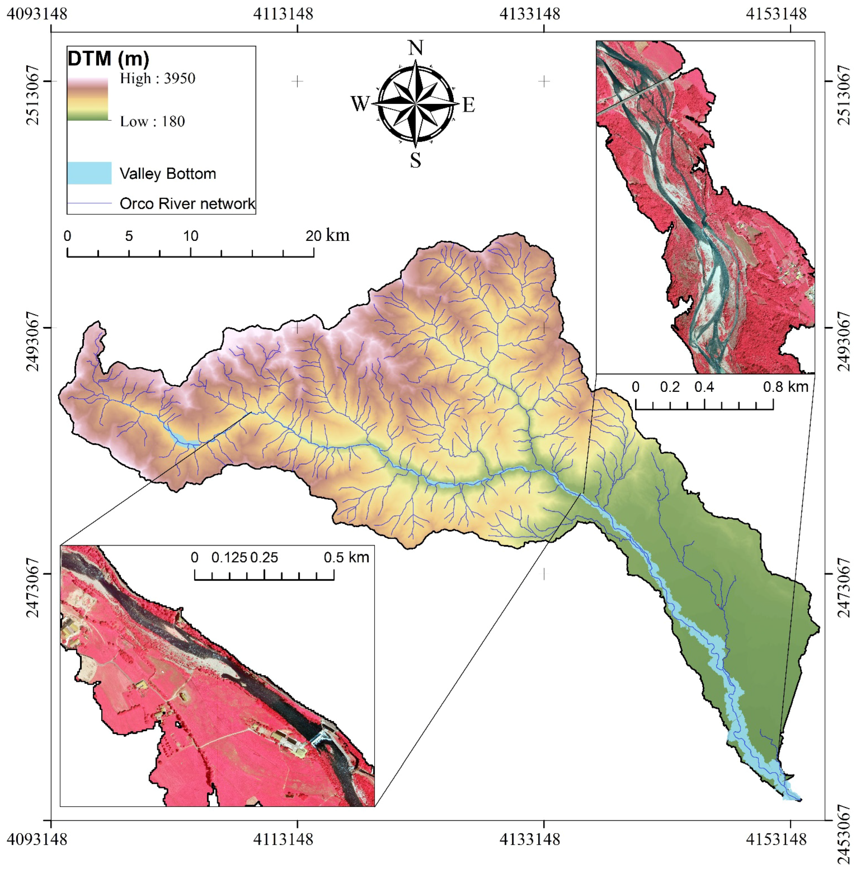
2.1. The Orco River
2.2. Classification Process: Riverscape Units and in-Stream Mesohabitats

| Land-Cover Class | Class Description | |
|---|---|---|
| Level 1 | Level 2 | |
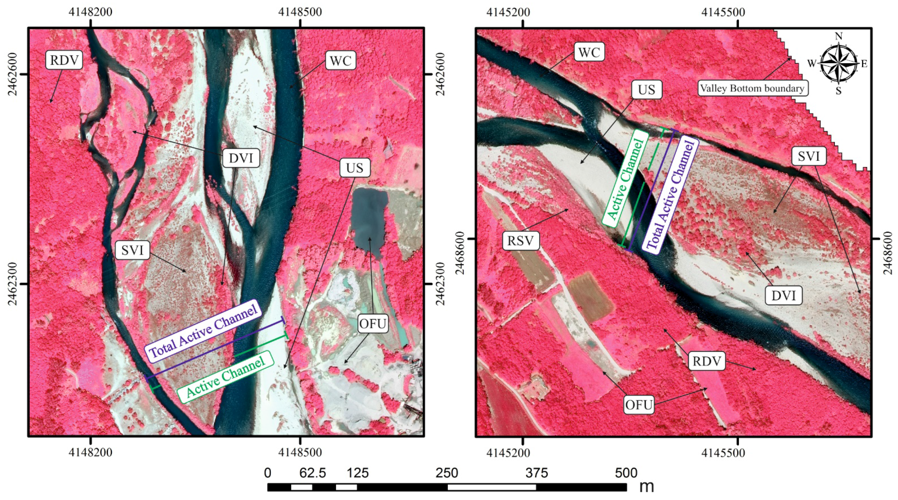
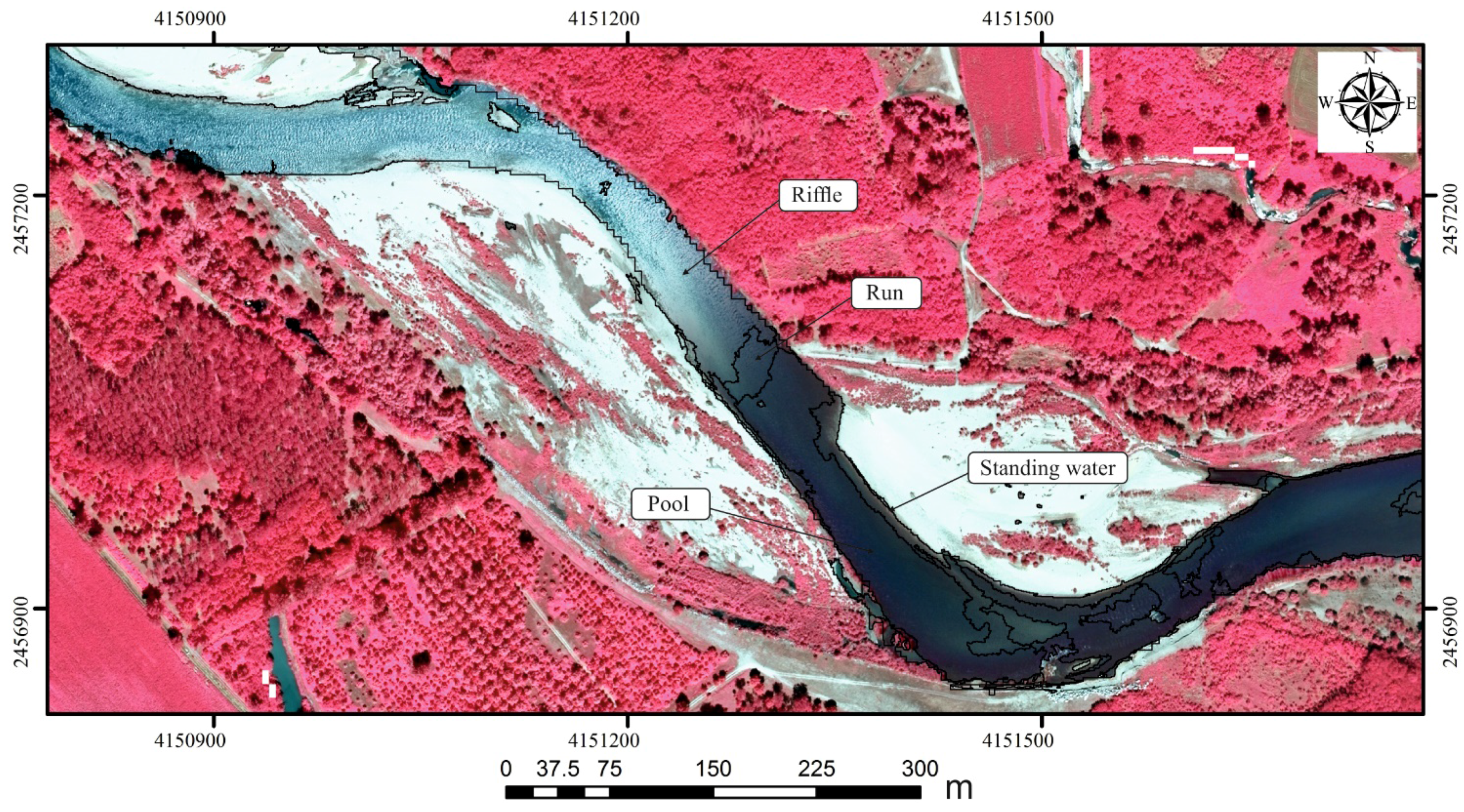
| Water Channel (WC)—part of the AC | Pools | Areas with a gentle surface slope and slow flow. |
| Riffles | Areas of swifter-flowing water. | |
| Runs | Areas of fast-moving, non-turbulent flow. | |
| Standing Waters | Surface water relatively still. | |
| Unvegetated Sediment bars (US)—part of the AC | Sediment bars without vegetation. | |
| Sparsely-Vegetated units (SV)—part of the Total Active Channel | Sparsely-Vegetated units of Islands (SVI) | Sparse vegetation units entirely surrounded by WC and/or US. |
| Riparian Sparsely-Vegetated units (RSV) | Riparian sparse vegetation units adjacent to (but not surrounded by) WC and/or US. | |
| FloodPlain units (FP) | Densely-Vegetated units of Islands (DVI) | Dense vegetation units entirely surrounded by WC and/or US and/or SVI. |
| Riparian Densely-Vegetated units (RDV) | Riparian dense vegetation units adjacent to (but not surrounded by) WC and/or US and/or RSV. | |
| Other Floodplain Units (OFU) | All remaining floodplain units | |


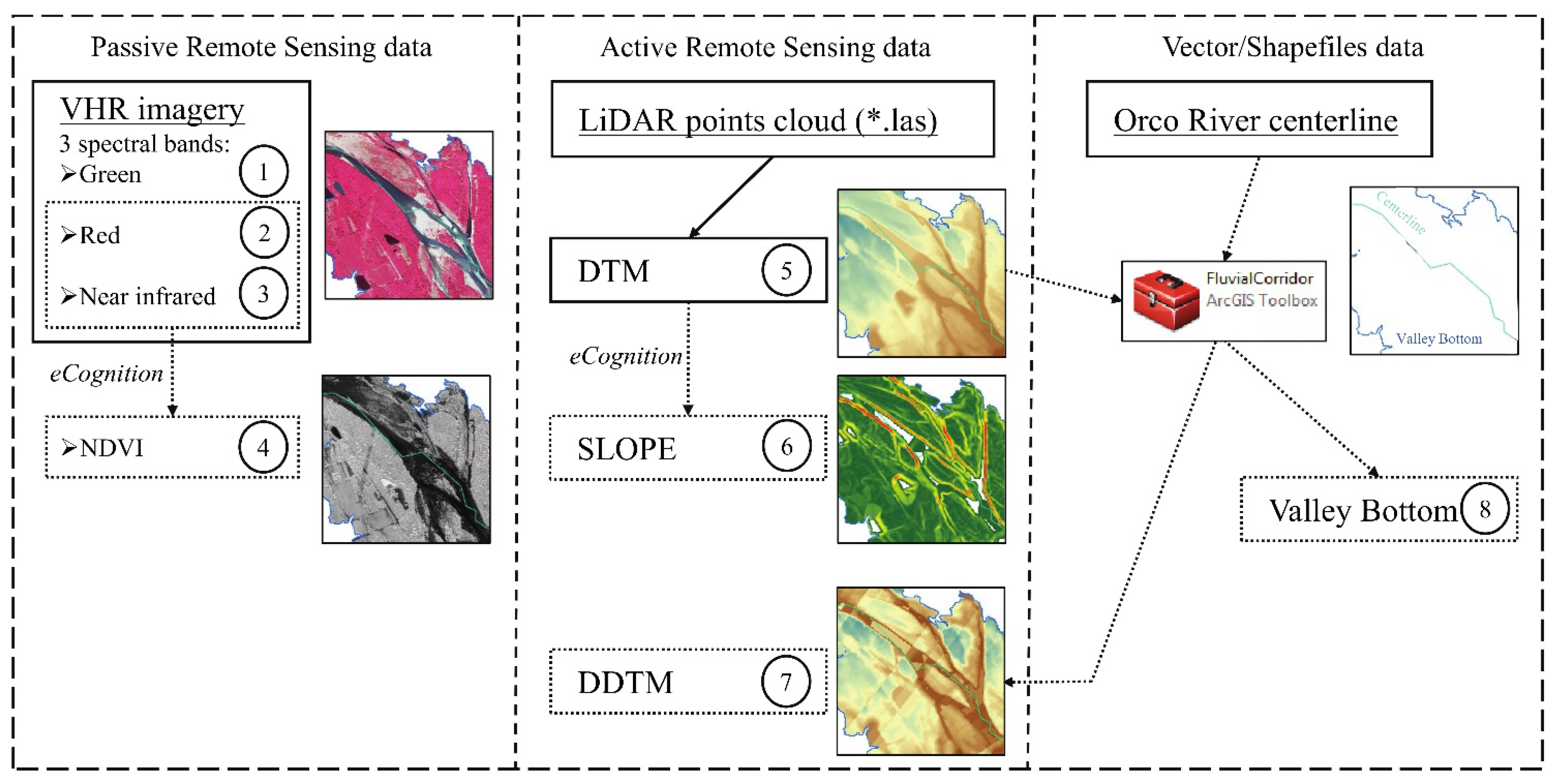
2.3. Remote Sensing and GIS Input Data Preparation
3. Methodology
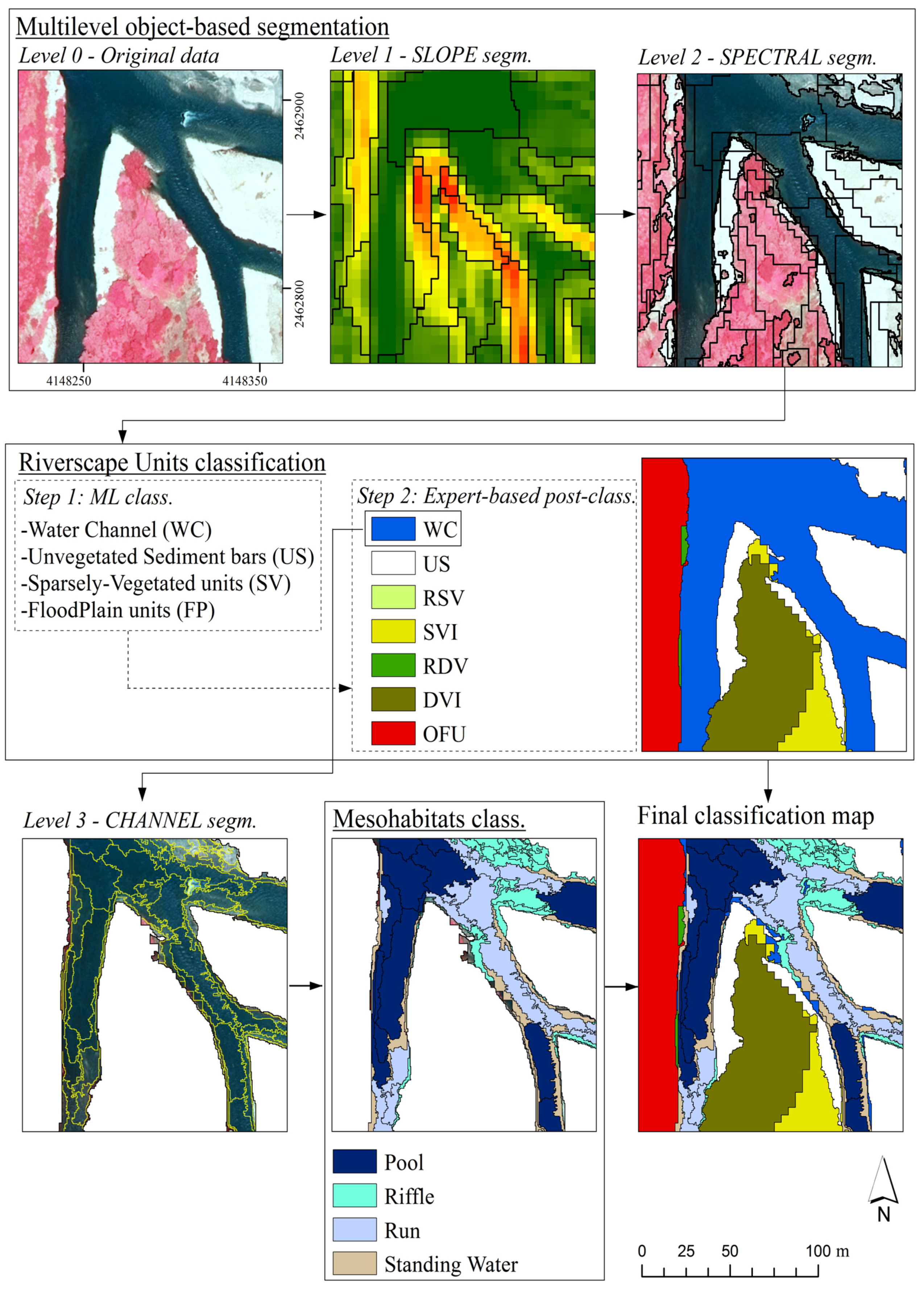
3.1. Multilevel GEographical Object-Based Image Analysis (GEOBIA)

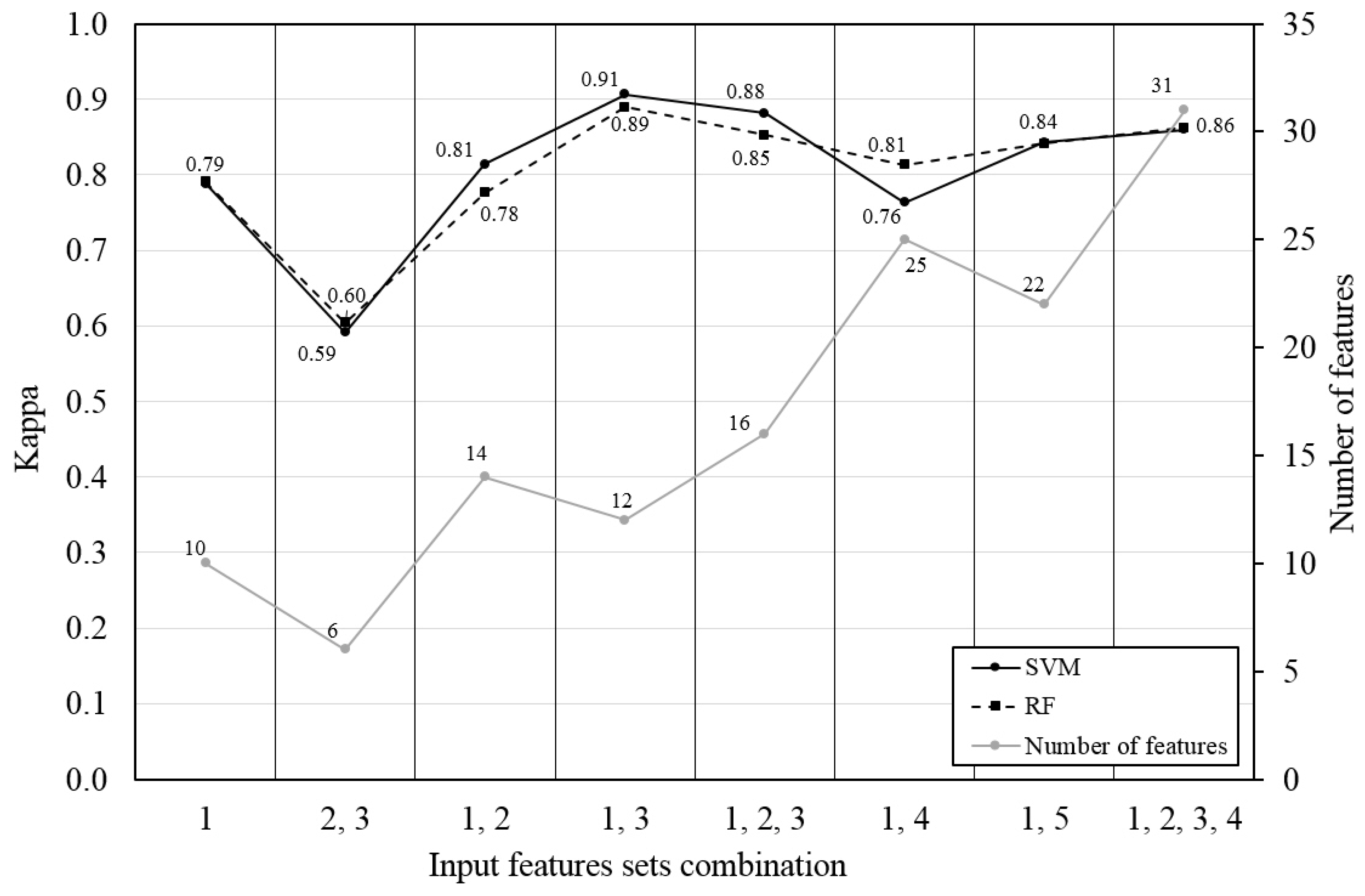
3.2. Multilevel, Machine Learning Classification of Riverscape Units and in-Stream Mesohabitats
| (1) VHR (10) | (2) LiDAR (4) | (3) DDTM (2) | (4) Geometric (15) | (5) Texture (12) |
|---|---|---|---|---|
| Mean: -Green -Red -Near infrared -NDVI Standard Deviation: -Brightness -Max difference -Green -Red -Near Infrared -NDVI | Mean: -DTM -SLOPE Standard Deviation: -DTM -SLOPE | Mean: -DDTM Standard Deviation: -DDTM | Area | Homogeneity (GLCM) |
| Border length | Contrast (GLCM) | |||
| Length | Dissimilarity (GLCM) | |||
| Length/Width | Entropy (GLCM) | |||
| Width | Angle of 2nd moment (GLCM) | |||
| Asymmetry | Mean (GLCM) | |||
| Border index | Standard deviation (GLCM) | |||
| Compactness | Correlation (GLCM) | |||
| Density | Angle of 2nd moment (GLDV) | |||
| Elliptic fit | Entropy (GLDV) | |||
| Radius of largest enclosed ellipse | Mean (GLDV) | |||
| Radius of smallest enclosing ellipse | Contrast (GLDV) | |||
| Rectangular fit | ||||
| Roundness | ||||
| Shape index |
| Training | Validation | |||||
|---|---|---|---|---|---|---|
| Samples | Area (km2) | % | Samples | Area (km2) | % | |
| WC | 2556 | 1.07 | 3.6 | 1504 | 0.92 | 3.1 |
| US | 2950 | 0.74 | 2.5 | 1990 | 0.73 | 2.4 |
| SV | 2919 | 0.74 | 2.5 | 1736 | 0.65 | 2.2 |
| FP | 21761 | 5.71 | 19.0 | 18827 | 4.56 | 15.2 |
| 27.5 | 22.9 | |||||
4. Results and Discussion
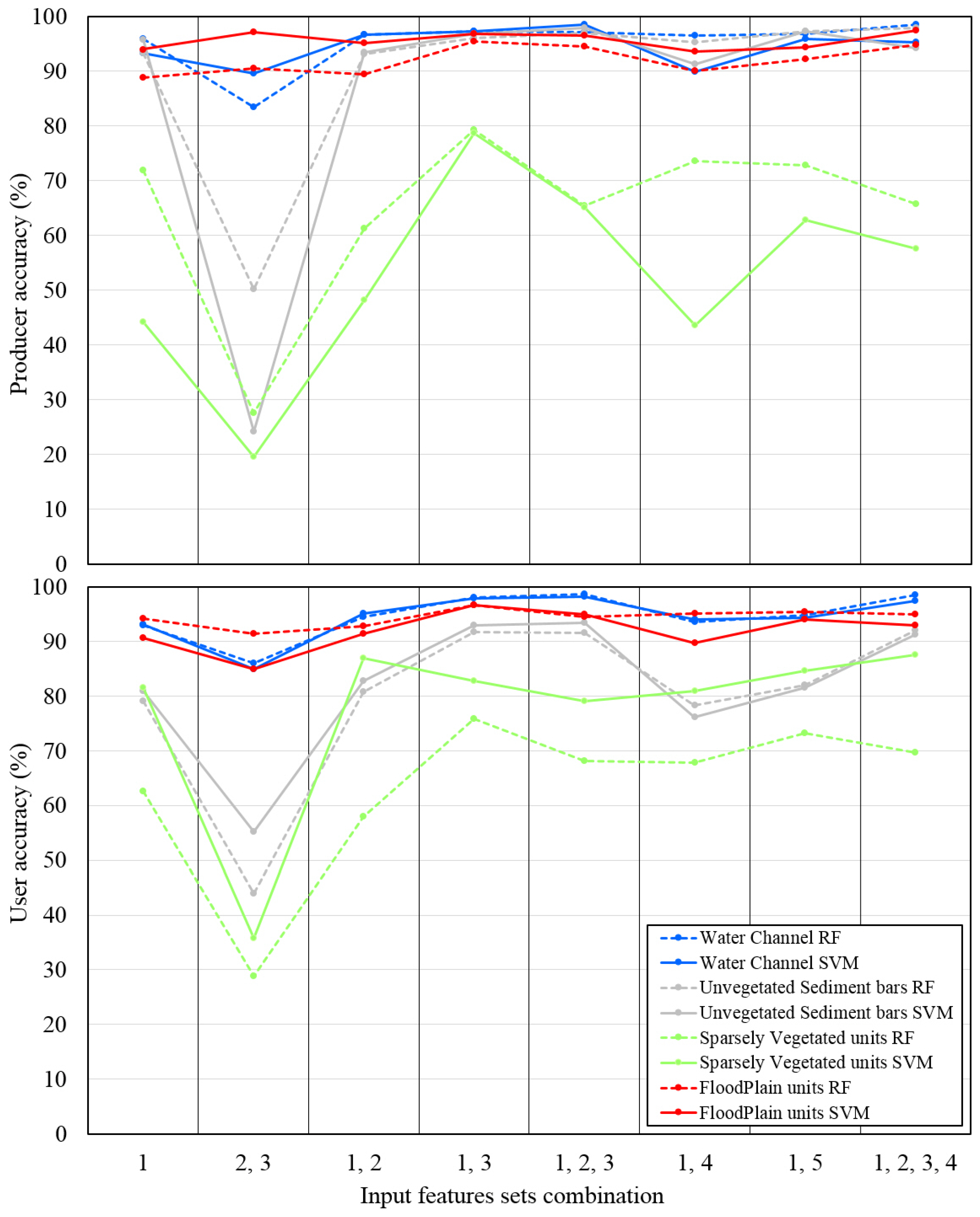
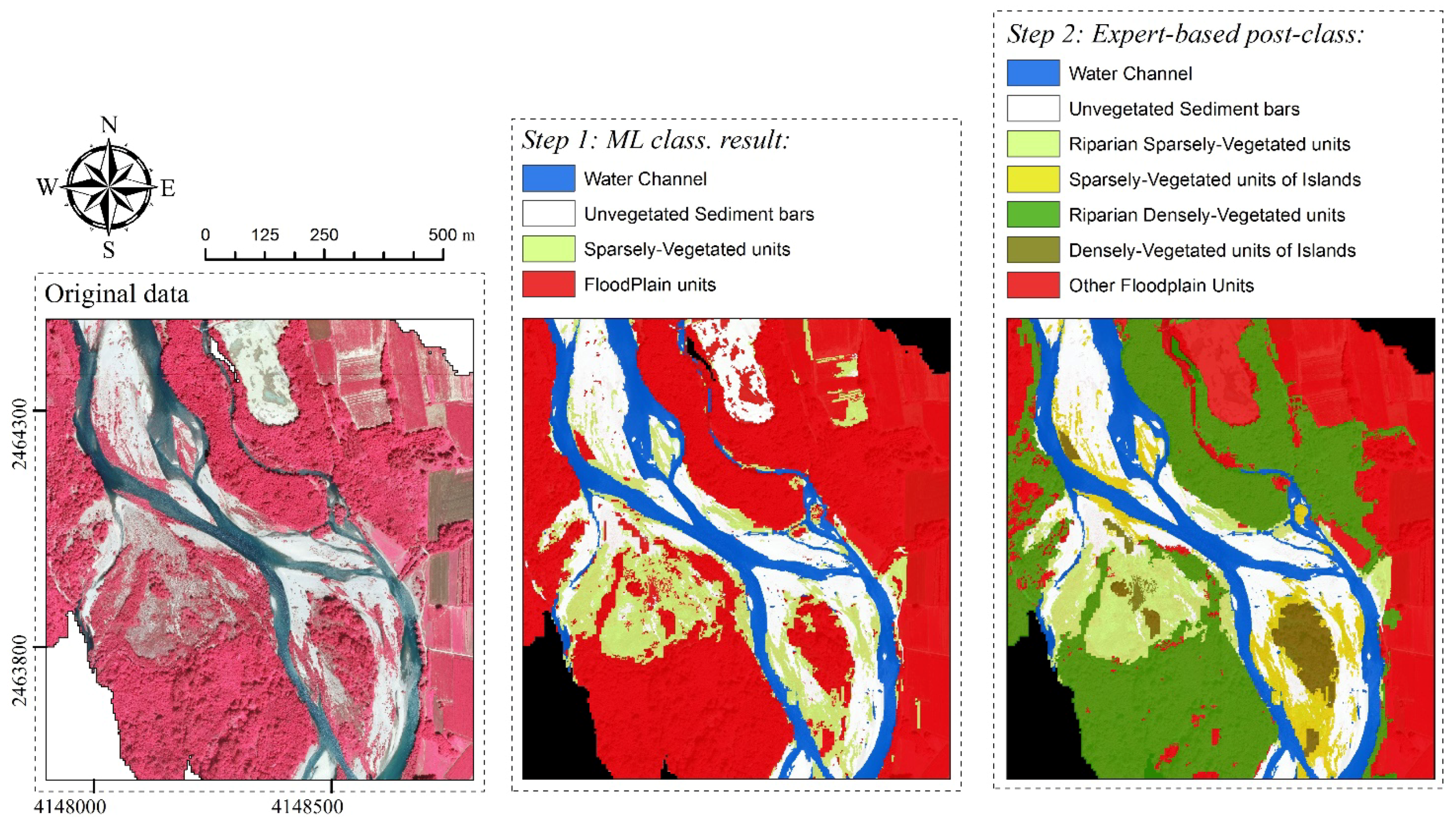
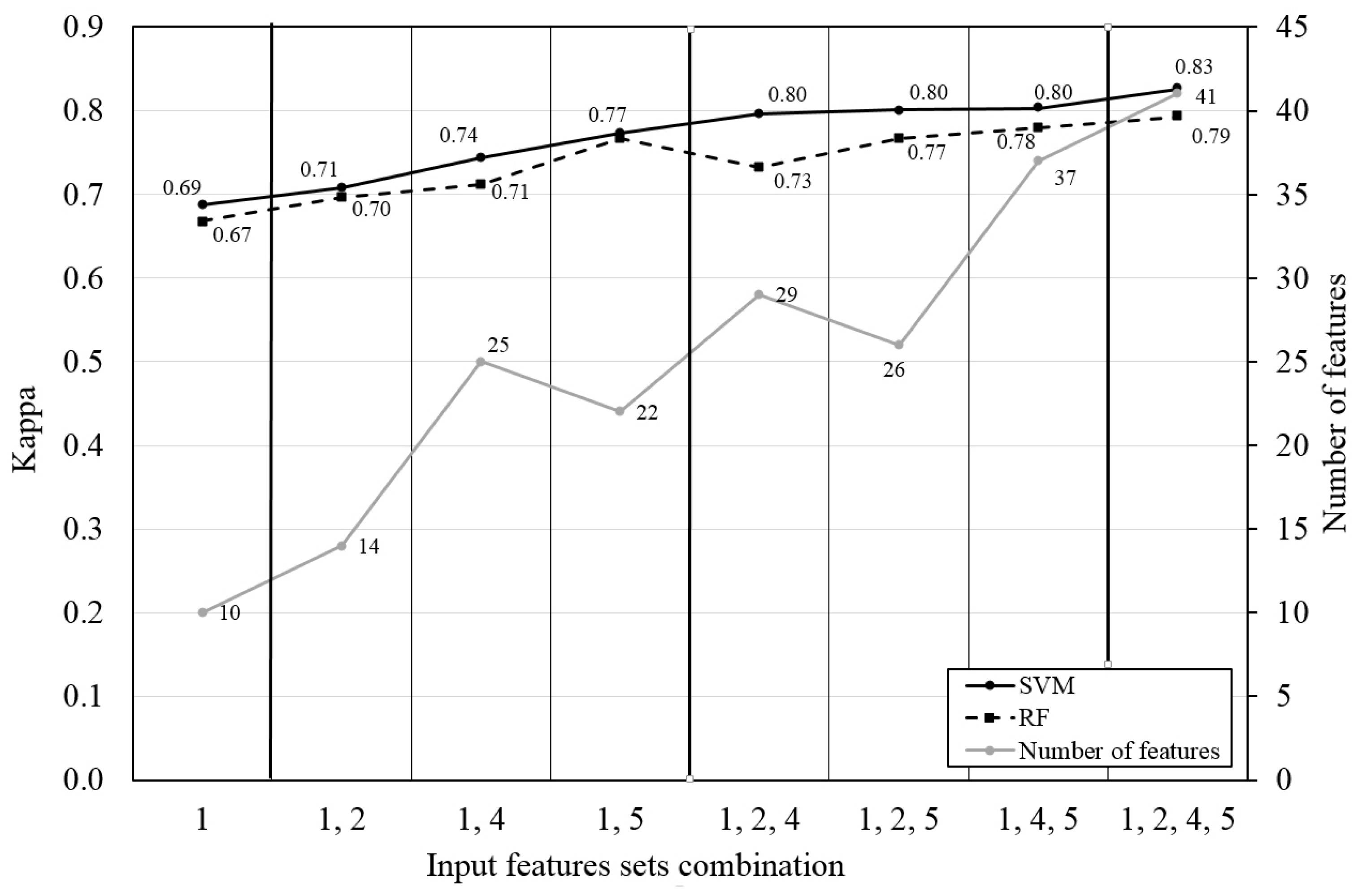
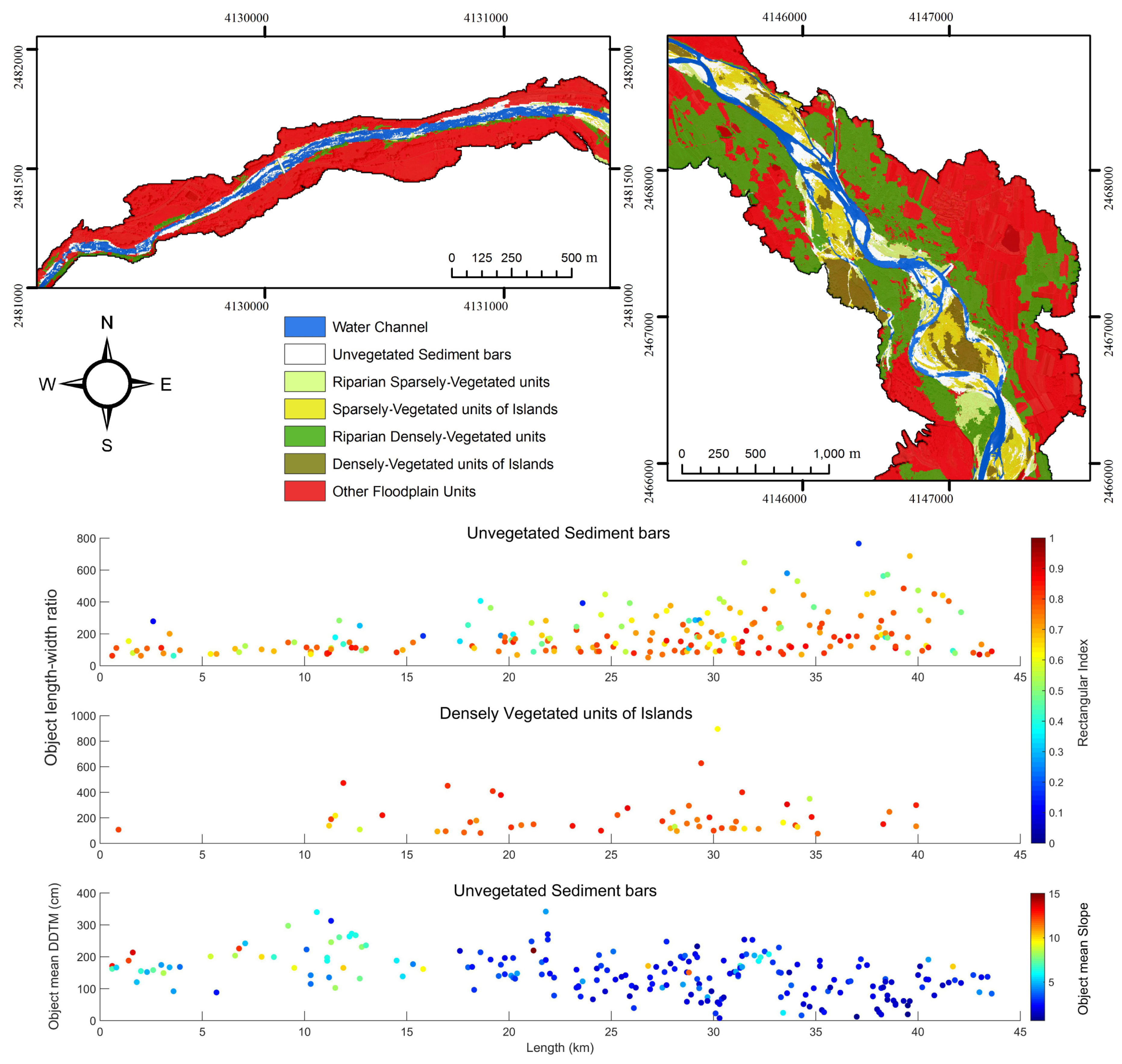
4.1. Riverscape Units Classification Results

| Total | FP | US | WC | SV | ||
|---|---|---|---|---|---|---|
| CE before post-classification | FP | 3.38 | - | 0.45 | 0.19 | 2.74 |
| US | 7.15 | 4.65 | - | 1.15 | 1.35 | |
| WC | 2.14 | 1.51 | 0.15 | - | 0.48 | |
| SV | 17.25 | 15.77 | 0.25 | 1.23 | - | |
| CE after post-classification | FP | 2.13 | - | 0.23 | 0.17 | 1.73 |
| US | 3.87 | 1.07 | - | 1.29 | 1.51 | |
| WC | 1.41 | 0.78 | 0.15 | - | 0.48 | |
| SV | 4.98 | 3.31 | 0.30 | 1.37 | - | |
| Total | FP | US | WC | SV | ||
|---|---|---|---|---|---|---|
| OE before post-classification | FP | 3.23 | - | 0.78 | 0.30 | 2.15 |
| US | 3.19 | 2.80 | - | 0.18 | 0.21 | |
| WC | 2.70 | 0.92 | 0.95 | - | 0.83 | |
| SV | 21.36 | 19.11 | 1.58 | 0.67 | - | |
| OE after post-classification | FP | 0.74 | - | 0.18 | 0.16 | 0.40 |
| US | 1.85 | 1.43 | - | 0.19 | 0.23 | |
| WC | 2.66 | 0.83 | 1.03 | - | 0.80 | |
| SV | 15.39 | 12.84 | 1.82 | 0.73 | - |

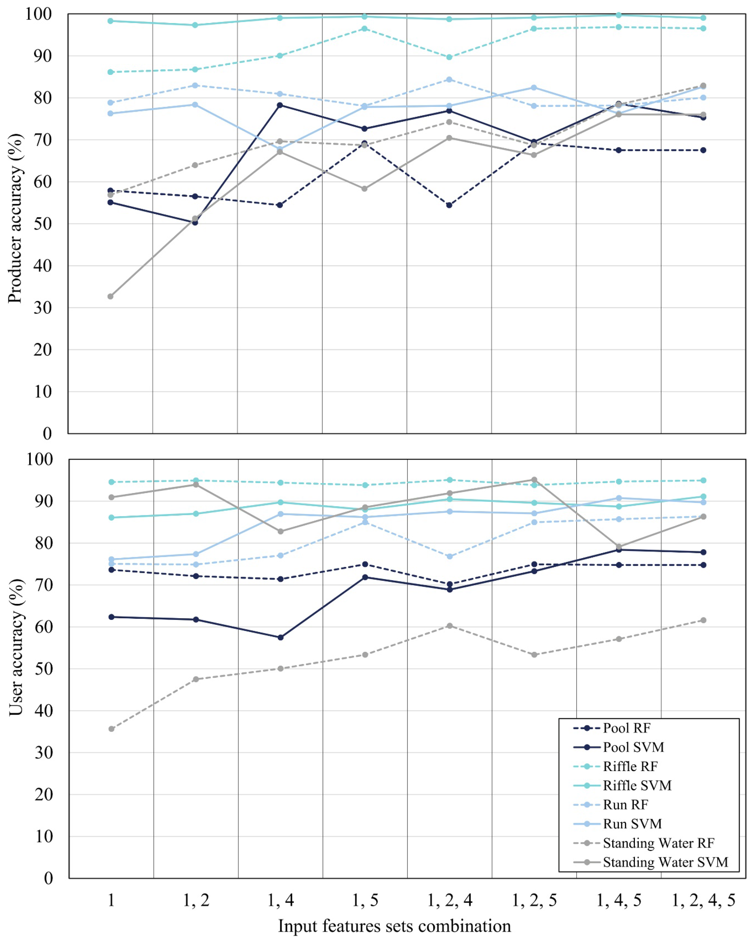
4.2. In-Stream Mesohabitat Classification Results


4.3. New Perspectives in Hydromorphological Characterization of Rivers

5. Conclusions
Acknowledgments
Author Contributions
Conflicts of Interest
References
- Brierley, G.J.; Fryirs, K.A. Geomorphology and River Management: Applications of the River Styles Framework; Blackwell: Oxford, UK, 2005. [Google Scholar]
- Rinaldi, M.; Surian, N.; Comiti, F.; Bussettini, M. A method for the assessment and analysis of the hydromorphological condition of Italian streams: The Morphological Quality Index (MQI). Geomorphology 2013, 180, 96–108. [Google Scholar] [CrossRef]
- Gurnell, A.M.; Rinaldi, M.; Belletti, B.; Bizzi, S.; Blamauer, B.; Braca, G.; Buijse, T.; Bussettini, M.; Camenen, B.; Comiti, F.; et al. A multi-scale hierarchical framework for developing understanding of river behaviour to support river management. Acquat. Sci. 2016, 78, 1–16. [Google Scholar]
- European Commission. Directive 2000/60/EC of the European Parliament and of the Council establishing a framework for Community action in the field of water policy. Off. J. Eur. Union 2000, 327, 1–73. [Google Scholar]
- Carbonneau, P.E.; Piégay, H. Fluvial Remote Sensing for Science and Management; Carbonneau, P.E., Piégay, H., Eds.; John Wiley & Sons, Ltd: Chichester, UK, 2012. [Google Scholar]
- Marcus, W.A.; Fonstad, M.A. Remote sensing of rivers: The emergence of a subdiscipline in the river sciences. Earth Surf. Process. Landf. 2010, 35, 1867–1872. [Google Scholar] [CrossRef]
- Buffington, J.M.; Montgomery, D.R. Geomorphic classification of river. In Treatise on Geomorphology; Shroder, J., Wohl, E., Eds.; Elsevier: San Diego, CA, USA, 2013; pp. 730–767. [Google Scholar]
- Bertrand, M.; Piégay, H.; Pont, D.; Liébault, F.; Sauquet, E. Sensitivity analysis of environmental changes associated with riverscape evolutions following sediment reintroduction: Geomatic approach on the Drôme River network, France. Int. J. River Basin Manag. 2013, 11, 19–32. [Google Scholar] [CrossRef]
- Alber, A.; Piégay, H. Spatial disaggregation and aggregation procedures for characterizing fluvial features at the network-scale: Application to the Rhône basin (France). Geomorphology 2011, 125, 343–360. [Google Scholar] [CrossRef]
- Belletti, B.; Dufour, S.; Piégay, H. What is the relative effect of space and time to explain the braided river width and island patterns at a regional scale? River Res. Appl. 2013. [Google Scholar] [CrossRef]
- Marcus, W.A.; Fonstad, M.A.; Legleiter, C.J. management applications of optical remote sensing in the active river channel. In Fluvial Remote Sensing for Science and Management; Carbonneau, P., Piegay, H., Eds.; John Wiley & Sons, Ltd.: Chichester, UK, 2012; pp. 19–42. [Google Scholar]
- Ham, D.; Church, M. Channel Island and Active Channel Stability in the Lower Fraser River Gravel Reach; University of British Columbia: Vancouver, BC, Canada, 2002. [Google Scholar]
- Toone, J.; Rice, S.P.; Piégay, H. Spatial discontinuity and temporal evolution of channel morphology along a mixed bedrock-alluvial river, upper Drôme River, southeast France: Contingent responses to external and internal controls. Geomorphology 2014, 205, 5–16. [Google Scholar] [CrossRef]
- Gurnell, A.M.; Petts, G.E.; Hannah, D.M.; Smith, B.P.G.; Edwards, P.J.; Kollmann, J.; Ward, J.V.; Tockner, K. Riparian vegetation and island formation along the gravel-bed Fiume Tagliamento, Italy. Earth Surf. Process. Landf. 2001, 26, 31–62. [Google Scholar] [CrossRef]
- Wintenberger, C.; Rodrigues, S.; Villar, M.; Bréhéret, J.G. The key role of pioneer woody vegetation in mid-channel bar metamorphosis to island: Case study from the River Loire (France). In Proceedings of the 10th International Conference on Fluvial Sedimentology, Leeds, UK, 14–19 July 2013; pp. 2–3.
- Osterkamp, W.R. Processes of fluvial island formation, with examples from Plum Creek, Colorado and Snake River, Idaho. Wetlands 1998, 18, 530–545. [Google Scholar] [CrossRef]
- Arnaud, F.; Piégay, H.; Schmitt, L.; Rollet, A.J.; Ferrier, V.; Béal, D. Historical geomorphic analysis (1932–2011) of a by-passed river reach in process-based restoration perspectives: The Old Rhine downstream of the Kembs diversion dam (France, Germany). Geomorphology 2015, 236, 163–177. [Google Scholar] [CrossRef]
- Piégay, H.; Darby, S.A.; Mosselmann, E.; Surian, N. The erodible corridor concept: Applicability and limitations for river management. River Res. Appl. 2005, 21, 773–789. [Google Scholar] [CrossRef]
- Bollati, I.M.; Pellegrini, L.; Rinaldi, M.; Duci, G.; Pelfini, M. Reach-scale morphological adjustments and stages of channel evolution: The case of the Trebbia River (northern Italy). Geomorphology 2014, 221, 176–186. [Google Scholar] [CrossRef]
- Liébault, F.; Piegay, H. Assessment of channel changes due to long term bedload supply decrease, Roubion River, France. Geomorphology 2001, 36, 167–186. [Google Scholar] [CrossRef]
- Legleiter, C.J. Remote measurement of river morphology via fusion of LiDAR topography and spectrally based bathymetry. Earth Surf. Process. Landf. 2012, 37, 499–518. [Google Scholar] [CrossRef]
- Wiederkehr, E.; Belletti, B.; Dufour, S.; Piégay, H. Physical characterisation of river corridors from orthophotos: Challenging issues and first application to the Rhône hydrographical network. In Proceedings of the GEOBIA 2010-Geographic Object-Based Image Analysis Conference, Ghent, Belgium, 29 June–2 July 2010; pp. 1682–1777.
- Vezza, P.; Parasiewicz, P.; Spairani, M.; Comoglio, C. Habitat modeling in high-gradient streams: The mesoscale approach and application. Ecol. Appl. 2014, 24, 844–861. [Google Scholar] [CrossRef] [PubMed]
- Frissell, C.; Liss, W.J.; Warren, C.E.; Hurley, M.D. A hierarchical framework for stream habitat classification: Viewing streams in a watershed context. Environ. Manag. 1986, 10, 199–214. [Google Scholar] [CrossRef]
- European Commission. Directive 1992/43/EEC on the conservation of natural habitats and of wild fauna and flora. Off. J. Eur. Union 1992, 389, 7–50. [Google Scholar]
- Acreman, M.C.; Ferguson, A.J.D. Environmental flows and the European Water Framework Directive. Freshw. Biol. 2010, 55, 32–48. [Google Scholar] [CrossRef]
- Vezza, P.; Goltara, A.; Spairani, M.; Zolezzi, G.; Siviglia, A.; Carolli, M.; Cristina Bruno, M.; Boz, B.; Stellin, D.; Comoglio, C.; et al. Habitat indices for rivers: Quantifying the impact of hydro-morphological alterations on the fish community. In Engineering Geology for Society and Territory—Volume 3 SE—75; Lollino, G., Arattano, M., Rinaldi, M., Giustolisi, O., Marechal, J.-C., Grant, G.E., Eds.; Springer International Publishing: Basel, Switzerland, 2015; pp. 357–360. [Google Scholar]
- Wright, A.; Marcus, W.A.; Aspinall, R. Evaluation of multispectral, fine scale digital imagery as a tool for mapping stream morphology. Geomorphology 2000, 33, 107–120. [Google Scholar] [CrossRef]
- Legleiter, C.J.; Marcus, W.A.; Rick, L. Effects of sensor resolution on mapping instream habitats. Photogramm. Eng. Remote Sens. 2002, 68, 801–807. [Google Scholar]
- Marcus, W.A.; Legleiter, C.J.; Aspinall, R.J.; Boardman, J.W.; Crabtree, R.L. High spatial resolution hyperspectral mapping of in-stream habitats, depths, and woody debris in mountain streams. Geomorphology 2003, 55, 363–380. [Google Scholar] [CrossRef]
- Weng, Q.; Hu, X.; Lu, D. Extracting impervious surfaces from medium spatial resolution multispectral and hyperspectral imagery: A comparison. Int. J. Remote Sens. 2008, 29, 3209–3232. [Google Scholar] [CrossRef]
- Demarchi, L.; Canters, F.; Chan, J.C.-W.; van de Voorde, T. Multiple endmember unmixing of CHRIS/Proba imagery for mapping impervious surfaces in urban and suburban environments. IEEE Trans. Geosci. Remote Sens. 2012, 50, 3409–3424. [Google Scholar] [CrossRef]
- Bizzi, S.; Demarchi, L.; Grabowski, R.; Weissteiner, C.; van de Bund, W. The use of remote sensing to characterise hydromorphological properties of European rivers. Aquat. Sci. 2016, 78, 57–70. [Google Scholar] [CrossRef] [Green Version]
- Regione Piemonte. Piano di Tutela Della Acque-Allegato Tecnico II.h/1-Bilancio Delle Disponibilità Idriche Naturali e Valutazione Dell’incidenza dei Prelievi; Regione Piemonte: Turin, Italy, 2004. [Google Scholar]
- Turitto, O.; Audisio, C.; Agangi, A. Il ruolo svolto da piene straordinarie nel rimodellare la geometria di un alveo fluviale. Ital. J. Quat. Sci. 2008, 21, 303–316. [Google Scholar]
- Pellegrini, L.; Maraga, F.; Turitto, O.; Audisio, C.; Duci, G.; Pavia, U.; Ferrata, V. Evoluzione morfologica di alvei fluviali mobili nel settore occidentale del bacino padano. Ital. J. Quat. Sci. 2008, 21, 251–266. [Google Scholar]
- Weng, Q. Remote sensing of impervious surfaces in the urban areas: Requirements, methods, and trends. Remote Sens. Environ. 2012, 117, 34–49. [Google Scholar] [CrossRef]
- Herold, M.; Roberts, D.A.; Gardner, M.E.; Dennison, P.E. Spectrometry for urban area remote sensing—Development and analysis of a spectral library from 350 to 2400 nm. Remote Sens. Environ. 2004, 91, 304–319. [Google Scholar] [CrossRef]
- Dennison, P.E.; Roberts, D.A.; Regelbrugge, J. Characterizing chaparral fuels using combined hyperspectral and synthetic aperture radar. In Proceedings of the 9th JPL Airborne Earth Science Workshop, Pasadena, CA, USA, 23–25 February 2000; pp. 119–124.
- European Commission. Directive 2007/2/EC of the European Parliament and of the Council of 14 March 2007 establishing an Infrastructure for Spatial Information in the European Community (INSPIRE). Off. J. Eur. Union 2007, 108, 1–14. [Google Scholar]
- Zevenbergen, L.W.; Thorne, C.R. Quantitative analysis of land surface topography. Earth Surf. Process. Landf. 1987, 12, 47–56. [Google Scholar] [CrossRef]
- Roux, C.; Alber, A.; Bertrand, M.; Vaudor, L.; Piégay, H. “FluvialCorridor”: A new ArcGIS toolbox package for multiscale riverscape exploration. Geomorphology 2015, 242, 29–37. [Google Scholar] [CrossRef]
- Notebaert, B.; Piégay, H. Multi-scale factors controlling the pattern of floodplain width at a network scale: The case of the Rhône basin, France. Geomorphology 2013, 200, 155–171. [Google Scholar] [CrossRef]
- Hay, G.J.; Castilla, G. Geographic object-based image analysis (GEOBIA): A new name for a new discipline. In Lecture Notes in Geoinformation and Cartography; Springer Berling Heidelberg: Heidelberg, Germany, 2008; pp. 75–89. [Google Scholar]
- Platt, R.V.; Rapoza, L. An evaluation of an object-oriented paradigm for land use/land cover classification. Prof. Geogr. 2008, 60, 87–100. [Google Scholar]
- Benz, U.C.; Hofmann, P.; Willhauck, G.; Lingenfelder, I.; Heynen, M. Multi-resolution, object-oriented fuzzy analysis of remote sensing data for GIS-ready information. ISPRS J. Photogramm. Remote Sens. 2004, 58, 239–258. [Google Scholar] [CrossRef]
- Breiman, L. Random forests. Mach. Learn. 2001, 45, 5–32. [Google Scholar] [CrossRef]
- Tzotsos, A.; Argialas, D. Support vector machine classification for object-based image analysis. In Object Based Image Analysis; Springer Berlin Heidelberg: Heidelberg, Germany, 2008; pp. 663–677. [Google Scholar]
- Xun, L.; Wang, L. An object-based SVM method incorporating optimal segmentation scale estimation using Bhattacharyya Distance for mapping salt cedar (Tamarisk spp.) with QuickBird imagery. GISci. Remote Sens. 2015, 52, 257–273. [Google Scholar] [CrossRef]
- Heumann, B.W. An object-based classification of mangroves using a hybrid decision tree—Support vector machine approach. Remote Sens. 2011, 3, 2440–2460. [Google Scholar] [CrossRef]
- eCognition Developer, Trimble. 9.0 User Guide; Trimble Germany GmbH: Munich, Germany, 2014. [Google Scholar]
- Haralick, R.M. Statistical and structural approach to texture. Proc. IEEE 1979, 67, 786–804. [Google Scholar] [CrossRef]
- Surian, N.; Rinaldi, M. Morphological response to river engineering and management in alluvial channels in Italy. Geomorphology 2003, 50, 307–326. [Google Scholar] [CrossRef]
- Belletti, B.; Dufour, S.; Piégay, H. Regional variability of aquatic pattern in braided reaches (example of the French Rhône basin). Hydrobiologia 2012, 712, 25–41. [Google Scholar] [CrossRef]
- Schmitt, R.; Bizzi, S.; Castelletti, A. Characterizing fluvial systems at basin scale by fuzzy signatures of hydromorphological drivers in data scarce environments. Geomorphology 2014, 214, 69–83. [Google Scholar] [CrossRef]
© 2016 by the authors; licensee MDPI, Basel, Switzerland. This article is an open access article distributed under the terms and conditions of the Creative Commons by Attribution (CC-BY) license (http://creativecommons.org/licenses/by/4.0/).
Share and Cite
Demarchi, L.; Bizzi, S.; Piégay, H. Hierarchical Object-Based Mapping of Riverscape Units and in-Stream Mesohabitats Using LiDAR and VHR Imagery. Remote Sens. 2016, 8, 97. https://doi.org/10.3390/rs8020097
Demarchi L, Bizzi S, Piégay H. Hierarchical Object-Based Mapping of Riverscape Units and in-Stream Mesohabitats Using LiDAR and VHR Imagery. Remote Sensing. 2016; 8(2):97. https://doi.org/10.3390/rs8020097
Chicago/Turabian StyleDemarchi, Luca, Simone Bizzi, and Hervé Piégay. 2016. "Hierarchical Object-Based Mapping of Riverscape Units and in-Stream Mesohabitats Using LiDAR and VHR Imagery" Remote Sensing 8, no. 2: 97. https://doi.org/10.3390/rs8020097
APA StyleDemarchi, L., Bizzi, S., & Piégay, H. (2016). Hierarchical Object-Based Mapping of Riverscape Units and in-Stream Mesohabitats Using LiDAR and VHR Imagery. Remote Sensing, 8(2), 97. https://doi.org/10.3390/rs8020097