Abstract
Modern satellite radiometers have many detectors with different relative spectral response (RSR). Effect of RSR differences on striping and the root cause of striping in sensor data record (SDR) radiance and brightness temperature products have not been well studied. A previous study used MODTRAN radiative transfer model (RTM) to analyze striping. In this study, we make efforts to find the possible root causes of striping. Line-by-Line RTM (LBLRTM) is used to evaluate the effect of RSR difference on striping and the atmospheric dependency for VIIRS bands M15 and M16. The results show that previous study using MODTRAN is repeatable: the striping is related to the difference between band-averaged and detector-level RSR, and the BT difference has some atmospheric dependency. We also analyzed VIIRS earth view (EV) data with several striping index methods. Since the EV data is complex, we further analyze the onboard calibration data. Analysis of Variance (ANOVA) test shows that the noise along track direction is the major reason for striping. We also found evidence of correlation between solar diffuser (SD) and blackbody (BB) for detector 1 in M15. Digital Count Restoration (DCR) and detector instability are possibly related to the striping in SD and EV data, but further analysis is needed. These findings can potentially lead to further SDR processing improvements.
1. Introduction
Suomi National Polar Orbiting Partnership (S-NPP) spacecraft was successfully launched on 28 October 2011 with the Visible Infrared Imaging Radiometer Suite (VIIRS), which provides capacities for operational environmental remote sensing for weather, climate and other environmental applications. In contrast to conventional imaging radiometers [1], a single scan for VIIRS M bands (16 detectors aligned in the along-track direction) has a slower scan rate than that of the traditional single detector, therefore the spatial resolution is enhanced without losing the signal-to-noise (SNR). However, “bow tie” deletion and imaging striping occurs as a trade-off to this multi-detector arrangement that must be dealt with [1]. An anomalous striping pattern has been observed in SNPP VIIRS sea surface temperature products [2,3,4]. These striping are assumed to be caused by differences in the detector-level RSR. Currently SST EDR team developed an adaptive destriping algorithm to improve the operational SST imagery, but this destriping algorithm does not solve the problem at the root cause. The VIIRS SDR team performed studies to investigate possible root causes. Padula and Cao [4] used MODTRAN to evaluate the brightness temperature difference caused by the difference between band averaged (which is used in the operations) and detector level SRF. However, some studies [5] indicate that the forward model MODTRAN does not reproduce spectral, angular, and water vapor dependencies with accuracies acceptable for SST analyses. In the current study, we analyze the striping using atmospheric radiative transfer models LBLRTM to support assessment of VIIRS TEB calibration variations due to atmospheric effects.
The SST EDR group reported that some striping patterns were observed in SST product, which is possibly caused by the difference between detector-level and band-averaged SRF for some thermal emissive bands (TEB). Since the radiance in the SDR operational process is retrieved using the band-averaged instead of the detector level SRF, the difference will affect the derived brightness temperature and therefore SST. The level 2 daytime VIIRS SST environmental data is retrieved from a Non-linear Split Window algorithm from VIIRS bands M15 and M16 [2,5]:
where ai (i = 0, 1, 2, 3) is the coefficient derived from regression, BT15 and BT16 are the observed brightness temperature in VIIRS bands M15 and M16. SSTguess is the simulated first guess SST, and θ is the sensor zenith angle. This algorithm will amplify the striping caused by BT15 − BT16 due to the multiplication with the factor a2 SSTguess greater than 1.0 over the tropical ocean, but not always the case for the ocean over the polar region, and propagates it to the SST products [2,5]. Coincidently, most SST striping are reported for the tropical regions. From the water vapor absorption spectrum [6], we can see that the water vapor absorption in band centered at 12 μm (VIIRS M16) is larger than that in band centered at 10.8 μm (VIIRS M15), so M16 is more sensitive to water vapor absorption, i.e., the atmospheric impact on the BT variation is more obvious than that in M15. The brightness temperature in M16 is colder than that in M15 due to more water vapor absorption in M16.
2. Methodology
The detector-level radiance simulated from a Radiative Transfer Model, measured Suomi NPP hyperspectral radiance data and onboard calibration data are analyzed to investigate the impacts of detector-level SRF difference on striping, possibility of atmospheric dependency, as well as detector stability.
2.1. Radiative Transfer Model
In a previous study [4], the detector-level radiance and brightness temperature were simulated using MODTRAN [7], which is a “narrow band model” atmospheric radiative transfer with a spectral resolution of 1 cm−1 for TEB bands. In comparison, the Line-By-Line Radiative Transfer Model (LBLRTM) is a more accurate and flexible radiative transfer model that can be used over the full spectral range from the microwave to the ultraviolet, providing the foundation for many radiative transfer applications [8,9]. LBLRTM calculations in the thermal infrared bands are recognized as a reference standard for intercomparisons of radiative transfer models [10]. LBLRTM has been widely used for a number of years as the foundation for retrieval algorithms. It is also used to train fast radiative transfer models used in Numerical Weather Prediction (NWP) assimilation systems and the Optimal Spectral Sampling model [11] implemented in the Joint Center for Satellite Data Assimilation (JCSDA) Community Radiative Transfer Model (CRTM).
LBLRTM can provide much finer spectral resolution such as at 0.01 cm−1, which is more accurate for validation purposes. High spectral resolution is critical to identify and separate the causes of RSR effects from other possible causes. In this work, we use the LBLRTM v12.2, which was released in October 2012. It uses the AER line parameter database (hereafter AER3.2) on the basis of the HITRAN 2008 line parameter [12]. The Voigt line shape is used at all atmospheric levels with an algorithm according to a linear combination of approximating functions. Line coupling in LBLRTM is modeled using the first-order perturbation approach [13]. LBLRTM incorporates the continuum model MT_CKD [14], which includes self- and foreign-broadened water vapor continua as well as continua for CO2, O2, N2, O3, and extinction due to Rayleigh scattering.
To cover a range of environment conditions for evaluating TEB calibration and SST striping, we selected sites under various atmospheric conditions to perform simulations using LBLRTM, which can characterize atmospheric effects on SNPP VIIRS TEB calibration due to variability in atmospheric conditions. The results from LBLRTM will be compared with that from MODTRAN, which can serve as cross-check among models and help better determine the VIIRS detector level calibration biases due to effects of atmospheric radiative transfer.
2.2. Detector Level RSR
VIIRS is a whiskbroom scanning radiometer with a large scan angle which covers 112.56° at the nominal altitude of 829 km. It has many detectors with slightly different Relative Spectral Response (RSR). However, the impact of RSR difference among detectors on imagery artifacts, as well as geographical retrieval uncertainties has not been well studied until recently. Figure 1 shows detector-level and band averaged RSR function in M15. Band M16 includes two detector arrays A and B with time delay integration (VIIRS Radiometric Calibration ATBD, 2014). M16A and M16B figures are similar to that of M15, so they are not shown here. From the figure, we can see that RSR is slightly different among 16 detectors, which will affect the radiance and hence the brightness temperature. The impact of the detector level variation on the imagery artifacts will be analyzed in Section 3 and Section 4.
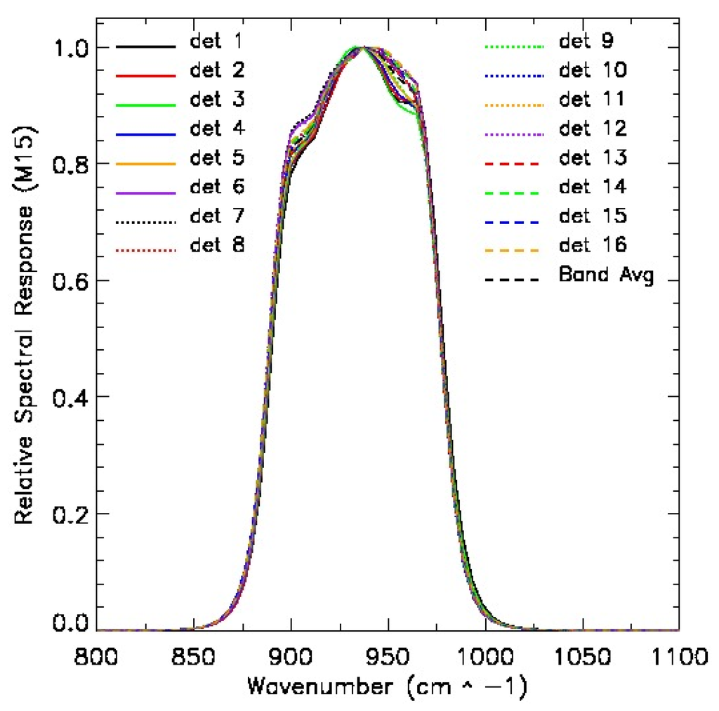
Figure 1.
Detector-level and band-averaged relative spectral response (RSR) in M15. Note: M16A and M16B figures are similar, not shown here.
2.3. Data Processing
LBLRTM v12.2 is used in this study to simulate the top of the atmosphere (TOA) radiance in the spectral range (722, 2650.0) cm−1 with spectral resolution of 0.01 cm−1. Six standard LBLRTM atmospheric profiles, including Tropical, Mid-Latitude Summer (MLS), Mid-Latitude Winter (MLW), Sub-Arctic Summer (SAS), Sub-Arctic Winter (SAW), and U.S. standard 1976 were used to ensure a broad range of simulated atmospheric conditions. The surface temperatures of 300 K, 290 K, 273 K, 280 K, 263 K, and 290 K were used for the above six atmospheres respectively.
The LBLRTM output TOA spectral radiance is then convolved with S-NPP VIIRS relative spectral response (RSR) to get the in-band averaged radiance mW/(m2·sr·cm−1):
where ν is the wavenumber, L(ν) is the at sensor radiance and RSR(ν) is the RSR at a given band. The computed in-band radiance (Lavg) can be converted to effective brightness temperature (Teff) by using the radiance to brightness temperature Look Up Tables. The original VIIRS LUT converts radiance in wavelength units to temperature. However, the spectral radiance output from LBLRTM is in the unit of W/(m2·sr·cm−1), so we used the temperature from VIIRS LUT to compute the spectral radiance in wavenumber unit using the Planck function and then convolve with spectral RSR to get the in-band radiance in wavenumber unit in order to match the unit from the model output which is in per wavenumber. By doing so, the interpolation is used to get finer spectral radiance versus BT LUT.
The blackbody radiance is computed from the Planck function:
where L(v,T) is the blackbody radiance (W/m2·sr·cm−1), c1 = 1.191042×10⁻⁸ (W/m2·sr·cm−1), c2 = 1.4387752 (K cm), v is the wavenumber (cm−1) and T is the blackbody temperature (K).
In this study, we can see that the expected striping is caused by the difference in effective brightness temperature (∆Teff) between the detector-level and band averaged RSR:
where Teff(det RSR) and Teff(avg RSR) are the effective brightness temperature computed using detector-level and band averaged RSR, respectively.
The striping due to detector level RSR difference can be defined as the difference in ∆Teff between two contiguous detectors i and i+1:
To evaluate the atmospheric dependencies, the simulated clear-sky radiance was processed using Equation (2) and detector level RSR to obtain the in-band radiance in M15 and M16. The radiance was then converted to effective brightness temperature for detector-level (Teff(det RSR)) and band averaged (Teff(avg RSR)) by using Look Up Tables. The brightness temperature difference ((∆Teff) was then computed from Equation (4) and the results are analyzed in next section.
3. Model Results and Discussion
Based on the above equations, Figure 2 shows the effective temperature difference between detector level and band averaged RSR for six LBLRTM atmospheres in M15, M16, and M15 − M16. As shown on the top left panel of Figure 2, in M15, we found that there is a small but obvious atmospheric dependency. The odd/even detector pattern is observed, especially for detectors 1 to 8. The smallest BT difference is at detector 5. The magnitude of variation is 0.01 K for tropical atmosphere, and 0.025 K for subarctic atmosphere. In order to see how the out-of-band response affects the temperature difference, we extend the spectral range from (800, 1100) cm−1 to the entire range (800, 1333.33) cm−1 in M15 and from (769, 950) cm−1 to (769, 1250) cm−1 in M16. After including the out-of-band response, the pattern in the temperature difference does not change much. The results (not shown) are similar to those of Figure 2. It is noted that the results from LBLRTM is similar to those in a previous study with MODTRAN [4].
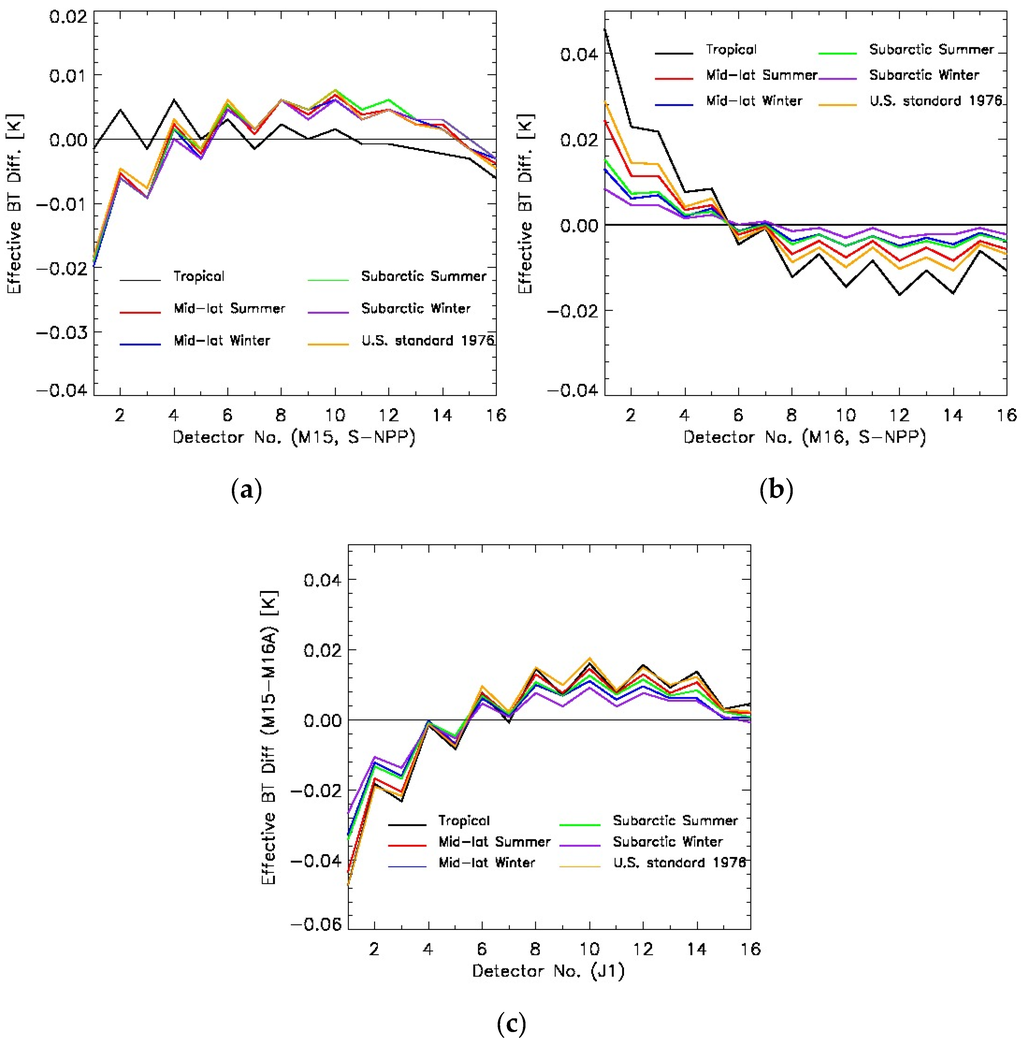
Figure 2.
Effective temperature difference between detector level and band averaged RSR for six line-by-line radiative transfer model (LBLRTM) atmospheres in M15 (a); M16 (b, the average of M16A and M16B); and M15 − M16 (c).
M16 is computed from the average of M16A and M16B and is shown in top right panel of Figure 2. There is more obvious atmospheric impact on BT difference than in M15, and the tropical atmosphere pattern has the largest variation. The magnitude of variation is 0.063 K for tropical atmosphere, and 0.022 K for subarctic atmosphere. We also observed apparent odd/even detector pattern. Figure 2b shows that in M16 band, detectors 1 and 2 deviate most from the band average than other detectors. The BTs for detectors 1−5 are larger than the band averaged value, but BTs for detectors 6, and 8−16 are smaller than the band average value. In Figure 2c, the BT differences (BT15 − BT16) from detectors 1−5 are smaller than the band average value, but they are larger than the band average for detectors 6−16. For detector 4 to 16, even if Sub-arctic Summer has higher temperature and more water vapor than Mid-latitude winter (see Table 1 [15]), but it doesn’t have higher variation, so striping is not always atmospheric dependent. Therefore, water vapor and temperature may not be the only cause for striping, and other instrument factors may also be involved, which was further explored later in the paper. After extending to the entire spectral range (800, 1333.33) cm−1 in M15 and (769, 1250) cm−1 in M16 to include the out-of-band response, the pattern is similar. Since the term (BT15 − BT16) is used in the VIIRS SST retrieval algorithm (Equation (1)), the difference between detector-level and band averaged BT in M15 − M16 should also be analyzed. The bottom panel of Figure 2 shows that the magnitude of variation in M15 − M16 is larger than that in single band, for example, they are 0.066 K and 0.063 K for tropical atmosphere in M15 − M16 and M16, respectively.

Table 1.
The dependence of atmospheric water vapor in the MODerate resolution atmospheric TRANsmission (MODTRAN) standard cases [15].
| Name | Columnar Liquid Water Equivalent (mm) |
|---|---|
| 1976 Standard Atmosphere | 17 |
| Tropical | 48 |
| Mid-latitude summer (MLS) | 35 |
| Mid-latitude winter (MLW) | 11 |
| Sub-arctic summer (SAS) | 25 |
| Sub-arctic winter (SAW) | 5 |
The ΔT in tropical atmosphere has larger magnitude (0.066 K) than subarctic (0.051 K). Compared to the band average, detectors 1−3 show larger atmospheric effect, with detector 1 showing the largest difference up to 0.046 K for tropical case, which is close to the 0.05 K in previous study [4] using MODTRAN model.
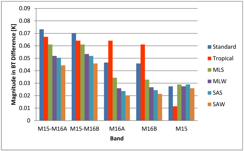
Figure 3.
The magnitude of brightness temperature difference (from Equation (4)) between using detector level and band averaged RSR for six LBLRTM atmospheres.
Figure 3 provides a summary of the magnitude in brightness temperature difference (Equation (4)) between using detector level and band averaged RSR from LBLRTM output for six atmospheres. It is shown that the magnitude in M15 − M16 is larger than that in single band. Comparing with M16 and M15 − M16, M15 is much less affected by atmosphere. Except for M15 and standard atmosphere, the magnitude has obvious atmospheric dependency: tropical region has much larger magnitude than subarctic region. We also noticed that although with larger temperature and liquid water content than MLW, SAS has a little bit smaller magnitude than MLW in M15 − M16 and M16. Therefore, besides water vapor and temperature, other instrument effects may also play a role in striping.
In general, the result from radiative transfer model indicates that LBLRTM does show atmospheric dependency although the difference is very small and is hard to validate. The water vapor has impact on the striping pattern in the satellite images. For example, in M16, the BT differences between using the detector-level and band averaged RSR are the largest for tropical atmosphere, and is the smallest for subarctic winter. The warm and moist atmosphere shows larger atmospheric impact on BT difference than the cold and dry atmosphere. The atmospheric impact is more obvious in band difference (M15 − M16) than for a single band. For example, the magnitude of ∆Teff for tropical atmosphere is 0.066 K, 0.063 K, 0.010 K in M15 − M16, M16, and M15, respectively. The magnitudes of ∆Teff for tropical and subarctic atmosphere are 0.066 K and 0.051 K in M15 − M16, and are 0.063 K and 0.024 K in M16. Compared to the band average, detector 1−3 shows large atmospheric effect, with detector 1 showing the largest difference up to 0.046 K for tropical case, which is close to the 0.05 K in previous study by Padula and Cao [4] using MODTRAN model. The impact of water vapor on the BT difference variation can be observed. In addition, other instrument effects may exist. The real satellite observation data are further analyzed in the next section to see whether the water vapor is a dominant factor affecting the striping pattern in the following sections.
4. Striping in VIIRS Earth Observation Data
In order to investigate the relationship between water vapor and striping in VIIRS brightness temperature images, The VIIRS SDR brightness temperature data for bands M15 and M16 are analyzed in sample cases from 2012 to 2014. Table 2 shows analysis of six cases over the “uniform” clear sky ocean surface near tropical and polar region. A major step forward in this study is that we experimented quantifying striping using different methods with more data samples.
Table 2.
Six cases used in this study.
| Cases | Granule |
|---|---|
| Tropical case 1: Bay of Bengal | d20130619_t0746444 |
| Tropical case 2: Bay of Bengal | d20140622_t0753301 |
| Tropical case 3: Bay of Bengal | d20140703_t0748470 |
| Polar case 1: Alaska | d20140520_t2158272 |
| Polar case 2: Alaska | d20140603_t2237573 |
| Polar case 3: Polar | d20150421_t1802552 |
4.1. Earth View Striping Quantification Using Cumulative Histogram Method
For each case, we selected a small uniform region with size of 60 pixels along scan direction, and 16 scan × 16 detector along track direction under clear sky condition according to VIIRS Cloud Mask Intermediate Product. Although the striping patterns can be observed from these images, it needs to be quantified with an index (named VSI). We used the cumulative histogram defined in previous studies [16,17] for striping quantification:
Where the first sum is to count the number of pixels with the value l (for detector i and HAM side A or B), and the second sum is over the pixel value l. In Equation (5), l can be BT or BT difference (BT15 − BT16), which depends on the striping index whether you want to quantify a single band or the band difference. The parameter in Equation (6) is the total number of the pixels in an image for the detector i and HAM side A or B. Here we didn’t separate the HAM side because we focus on the detector level RSR difference instead of HAM side difference in this study. refers to the percentage of the pixels with value less than k in an image. If there is striping pattern in an image, the histogram diverges for different detectors. The divergence of the histogram can be represented as the horizontal distances among the different histograms:
where P is the percentage of the pixels with the value less than the value in X-axis. X-axis represents the brightness temperatures (BT) or BT difference (BT15 − BT16).
The larger distance among different histogram corresponds to the stronger striping effects. We have analyzed the difference among 16 detectors (without separating HAM sides) for each small region.
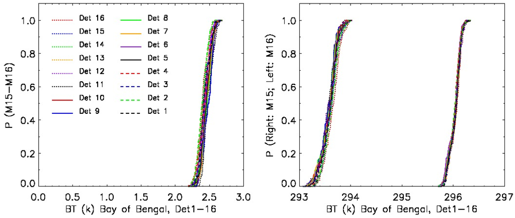
Figure 4.
The cumulative histogram for Bay of Bengal over tropical region on 19 June 2013 in M15 − M16 (left), as well as M15 and M16 (right).
In Figure 4, the Y-axis is the percentage of the pixels with the value less than the value in X-axis. In left panel, X-axis represents the brightness temperatures difference (BT15 − BT16). In the right panel, the values in X-axis are BT15 or BT16. Each line is for one detector. In this figure, we can see that the horizontal distance between histograms is almost a constant. Due to the water vapor absorption difference between M15 and M16, BT15 − BT16 can also represent the water vapor content. In M15 − M16, the maximum horizontal distance at 50% percentage is 0.093K, and the BT difference range is 0.5 K in X-axis. The following relative magnitude, i.e., the ratio of horizontal distance to the X-axis range, is better used to compare among different bands:
The ratio in M15 − M16, M15 and M16 are 0.187, 0.067 and 0.107, respectively. M15 − M16 has larger ratio than single band. These horizontal distances are larger than those from LBLRTM calculations by 0.027 K, 0.03 K, and 0.037 K in M15 − M16, M15, and M16, respectively. The large variation mainly comes from detector 1.
To better understand the atmospheric effect on striping, we have also analyzed the cases over the polar region. For example, Figure 5 shows the cumulative histogram over Gulf of Alaska on 20 May 2014 in M15 − M16 (left), as well as M15 and M16 (right). In general, the horizontal distance is very small and almost a constant. The ratios are 0.149, 0.044, and 0.015 in M15 − M16, M15 and M16, respectively, which are all smaller than those over topical cases. The histogram divergence in M15 − M16 is very close to the magnitude from LBLRTM, but is larger than LBLRTM magnitude by 0.023 K for M15 and less than LBLRTM by 0.005 K for M16. Polar region has smaller BT difference than tropical region due to smaller water vapor effect.
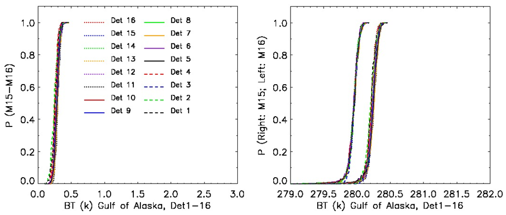
Figure 5.
Cumulative histogram over the Gulf of Alaska on 20 May 2014 in M15 − M16 (left), as well as M15 and M16 (right).
In this study, we have performed analysis on several cases, including three cases over tropical region and three cases over polar region (see Table 2). Figure 6 compares the magnitude of temperature variation among 16 detectors from VIIRS observation data and LBLRTM over tropical and polar region. In M15 − M16 and M16, both LBLRTM and VIIRS observation show larger temperature difference over tropical than over polar region, which means that the tropical region is much more affected by water vapor than polar region because the higher BT (larger than 2 K) difference in tropical region means more water vapor content. In most cases, VIIRS observation has larger magnitude in BT difference among different detectors than LBLRTM except for polar case 3 in M15 − M16. The maximum magnitude differences between VIIRS observation and LBLRTM for tropical cases are 0.028 K, 0.039 K, and 0.06 K in M15 − M16, M16, and M15, respectively. However, the magnitude difference between VIIRS observation and LBLRTM for polar case is less than 0.026 K.
In order to see whether the striping pattern is apparent in an image, the temperature range needs be considered, so the relative magnitude, i.e., the ratio of BT variation magnitude to temperature range, is compared over tropical and polar region (Figure 7). The results indicate that M15 − M16 has smaller temperature variation range than single band (M15 or M16), so the larger relative magnitude represents more obvious striping pattern in M15 − M16 image. The striping pattern in the image of BT15 − BT16 is more obvious than that in M15 or M16 because the signal to noise ratio (SNR) in the band difference image is larger than that in a single band. In most cases, the ratio in tropical region is larger than that over polar region except for tropical case 1. However, observation data has large variability and the variation cannot be effectively validated. In addition to water vapor, other factors such as instrument stability possibly affect the striping pattern.
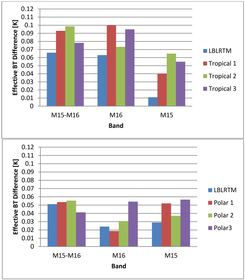
Figure 6.
The magnitude of brightness temperature variation among 16 detectors for Visible Infrared Imaging Radiometer Suite (VIIRS) observation data and LBLRTM over tropical (top) and polar (bottom) region for six cases.
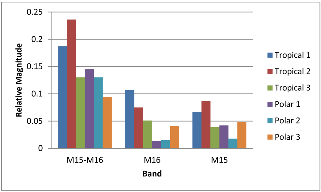
Figure 7.
Comparison of the relative magnitude (i.e., ratio of brightness temperature variation magnitude to temperature range) over tropical and polar region.
So far the striping pattern has been analyzed using LBLRTM and VIIRS observation data. Figure 8 compares the averaged effective temperature difference from LBLRTM and VIIRS observation. The results from observation are the averaged over several cases for both tropical and polar atmospheres. In M15 − M16 and M16, both LBLRTM and VIIRS observation show larger temperature difference in tropical than in polar region. In most cases, VIIRS observation has larger magnitude in temperature difference among different detectors than LBLRTM except for polar case in M15 − M16. For tropical atmosphere, VIIRS observation has larger magnitude than LBLRTM by 0.024 K in M15 − M16 and 0.025 K in M16. For polar atmosphere, the difference between observation and LBLRTM is 0.005 K in M15 − M16 and 0.009 K in M16. In general, the magnitude of variation among 16 detectors over tropical region is much more affected by water vapor than that over polar region, i.e., larger for high BT difference BT15 − BT16 (high water vapor absorption). Therefore, the water vapor has an impact on the striping pattern, but it is not the only factor.
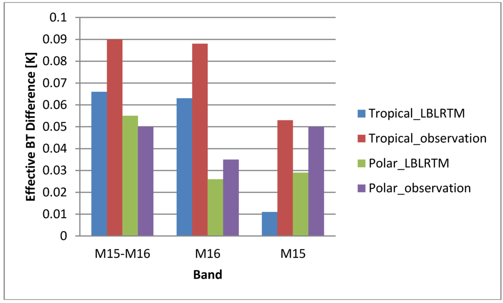
Figure 8.
Comparison of effective temperature difference between LBLRTM and the VIIRS observation for tropical and polar cases. Note: VIIRS observation uses the average of several cases to represent the tropical and polar case.
Based on the analysis above, we can see that LBLRTM results are nearly identical to the previous study using MODTRAN [4]. We found that results from MODTRAN are repeatable using LBLRTM. Previous study does not completely solve the problem because there are still some other potential factors related to striping issue, therefore we will look further on detector stability.
Alternatively, we have also used the definition of VIIRS striping index (VSI) as the ratio between the mean along-track variance () and the mean along scan variance ().
The results show that the VSI is very sensitive. It decreases from 5 to 0.4 as the number of samples increases from 10 to 60, and increases from 4 to 10 when the number of scans increases from 6 to 10. This method is further improved later for onboard data analysis.
When the mean changes with the orbit time, the Allan deviation [18] will be an appropriate method to describe the spread distribution of the measurement essentially. The Allan deviation is used to compute the variance along track and along scan direction, and then use the variance ratio of along track to along scan to represent the VSI. Comparing with the standard deviation method, this Allan deviation is not sensitive to the number of samples, but it is also not an ideal method to separate tropical and polar cases in striping quantification because there is no obvious difference in VSI between tropical and polar cases using this method.
In general, we have used three different methods, including cumulative histogram, standard deviation, and Allan deviation, to quantify VSI in earth view (EV) observation data. Among them, the cumulative histogram method is the best to use without strict limitations. The Allan deviation method is not very sensitive to the sample size of subset but is hard to separate the tropical and polar cases for striping quantification. The standard deviation method is sensitive to the sample size of earth view data, but it will be further improved for onboard data analysis in the following section. The earth view data is complex because the noise is mixed with signal, so we further analyze the onboard calibration data in the next section, which is spatially uniform and eliminates EV effect such as atmospheric effect.
4.2. VIIRS Striping Analysis Using Onboard Calibrated Data
The SDR radiometric calibration algorithms convert raw data record (RDR) from Earth View (EV) observations into SDR radiance, reflectance, and brightness temperature products using onboard calibrators. The VIIRS on board calibrators include Blackbody (BB), Solar Diffuser (SD), and Solar Diffuser Stability Monitor (SDSM). This two-point calibration approach uses two calibration points: the Onboard Calibration BB and SD as the high points for thermal emissive bands (TEB) and reflective solar bands (RSB), respectively, and Space View (SV) for offset subtraction for both bands. The instrument gain can be derived from VIIRS observations at these two calibration points, which provides the basis for the two-point non-linear calibration for TEBs. The BB temperature is accurately measured with six embedded BB thermistors. While majority of the blackbody radiance observed by a given band is emitted and its in-band spectral radiance calculated from the Planck function using BB thermistor temperatures, a small portion is due to thermal emission and reflection from several optical path and surrounding components: including the Rotating Telescope Assembly (RTA), Half Angle Mirror (HAM), scan cavity, and shield. In addition, the response versus scan angle effects (RVS) must also be considered [19].
A. Noise Analysis Using Raw Data from BB, SV, and SD
The detector noise based on BB, SV, and SD observations are analyzed. BB is a calibration source for TEB and it is spatially uniform. It can measure the noise of single detector along scan direction, and noise of different detectors along track direction. Each detector has its own gain, the change in gain and offset between scans, the Digital Count Restoration (DCR) or detector instability can lead to striping. DCR is the process to ensure that the lowest level signals never drop below the dynamic range of the Analog to Digital Converter (ADC).
The SD is originally designed as a calibration source for RSB. However, in this study, we use the SD as a calibrated target. The advantage is that it acts as a proxy for SST and can simulate the effect on SST. On the other hand, the SD temperature drifts and changes with time or orbit, so we will use the ratio of SD in HAM side A to B to remove this effect and perform analysis of variance. Now the standard deviation discussed before can be used for the SD radiance ratio. We have analyzed three continuous OBCIP files on 30 June 2015. Figure 9 indicates the variations of BB−SV (i.e., dBB) and SD−SV (i.e., dSD) along track and along scan directions for detector 1 in band M15. There are 48 samples and 72 scans for three granules. The patterns are more consistent along scan. The variation along track is much larger than that along scan, which suggests that it is an important factor causing the striping pattern.
The drifting trend of solar diffuser can also be shown clearly by comparing the pattern between BB−SV (i.e., dBB) and SD−SV (i.e., dSD) along track and along scan (Figure 10). For both dBB and dSD, the pattern within each scan is more consistent. The mean value of dSD increases with the time/orbit, which will be considered in the following analysis.
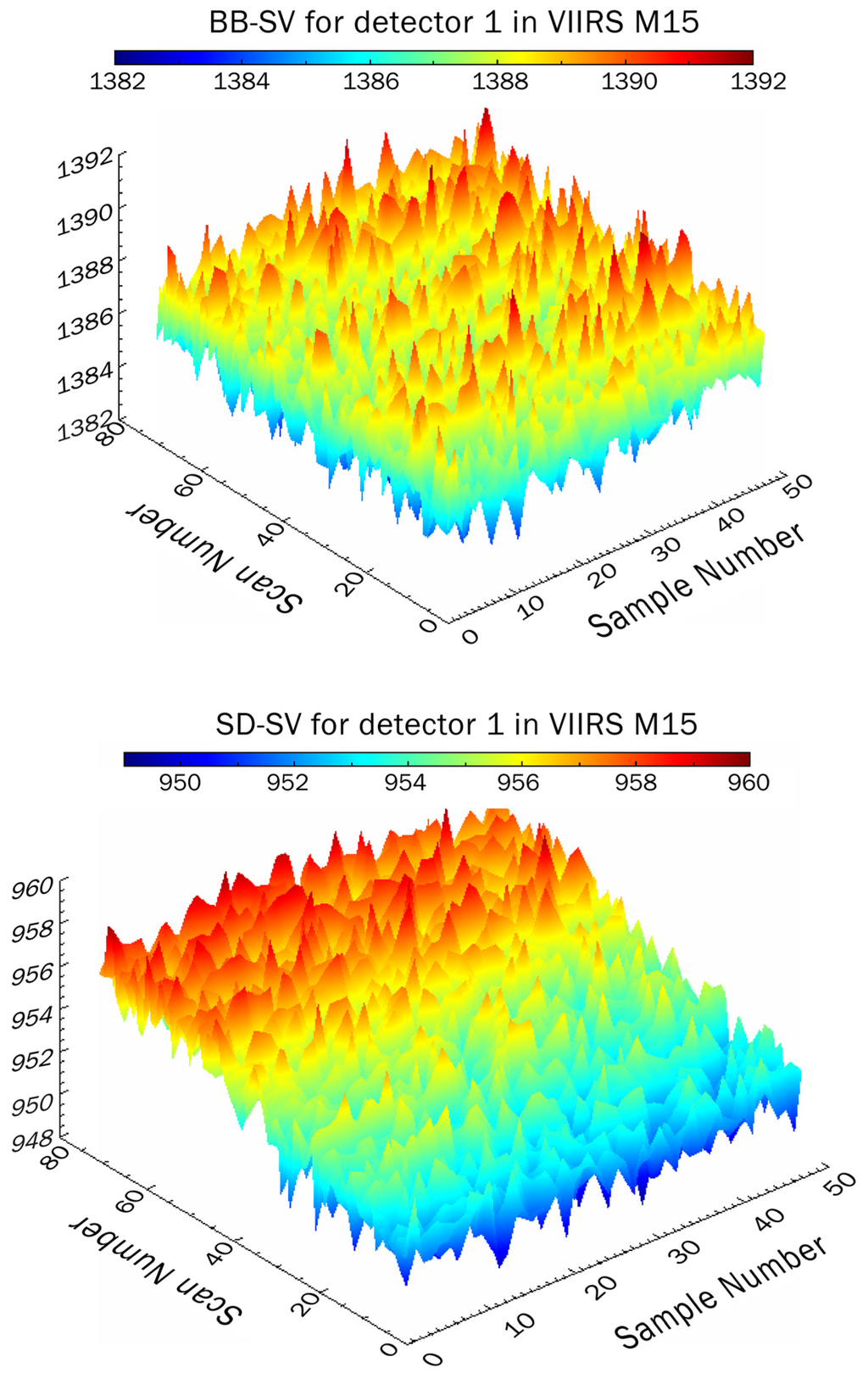
Figure 9.
Variations of BB−SV (i.e., dBB; top) and SD−SV (i.e., dSD; bottom) along track and along scan for detector 1 in M15.
The VIIRS observations of the BB includes the signal from the blackbody emitted radiance at the temperature measured by the platinum resistance thermistors (PRT), as well as instrument radiometric noise. If we assume the BB target and environment to be stable, then the variation of dBB can be mostly due to random noise, detector and DCR instability, (gain is assumed stable short term). The random noise effect can be illustrated by the variation of dBB with 48 samples from each scan, and the effect of DCR and detector change can be observed by the variation of dBB in along track direction. As an example, three continuous granules (t0755_e0756, t0756_e0758, and t0758_e0759) on 30 June 2015 are analyzed. Figure 11 provides the effects of random noise and DCR in M15. The black dashed lines in the figure refer to the averaged value. In the bottom panel, the variation of dBB with scan for detector 1 and 1st sample along track shows larger deviation from the averaged value, and the STD is 1.12612. In the top panel, the STD for dBB of 48 samples along scan direction is about 0.93589, which means the DCR is a dominant factor causing variation in dBB.
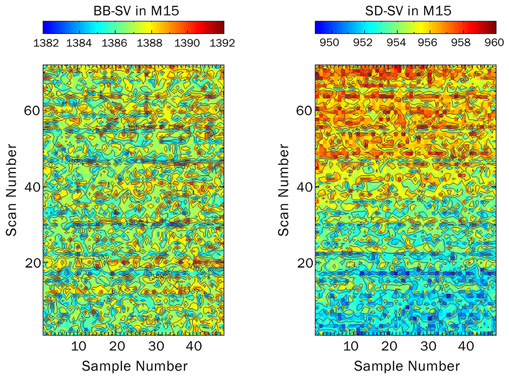
Figure 10.
The distribution of BB−SV (i.e., dBB; left) and SD−SV (i.e., dSD; right) for detector 1 in M15. Color represents the value of data.
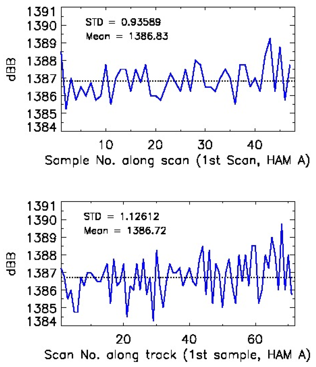
Figure 11.
The variation of dBB with 48 samples for one scan (top) and the variation of dBB with scan for detector 1 and 1st sample along track (bottom) in M15 for three continuous granules (t0755_e0756, t0756_e0758, and t0758_e0759) on 30 June 2015. Dashed line refers to the averaged value.
Analysis of variance (ANOVA) uses the standard deviation method to separate the overall variance into variations among and between groups, and then compare the ratios to determine the dominant statistical effect. Previously we mentioned that the standard deviation method cannot be applied to SD radiance directly because it has trend over the orbital time. However, after removing the drift trend by taking the HAM side ratio, it removes the trend and now we can use the two-way ANOVA method to evaluate the variation in SD radiance ratio along track and along scan directions. This method is not used for EV data analysis because EV data is complicated. When considering the ratio of two HAM sides, each detector has 24 scans and 48 samples in one granule OBCIP file. As an example, we analyzed two continuous granules on 30 June 2015, then each detector totally has 48 scans () and 48 samples () in these two granules. The following equations are used for the variance analysis of the SD radiance ratio ():
The mean square between scans is
The mean square between samples is
The mean square for error is
The ANOVA test ratio (V) along track and along scan are defined as
Where r is the number of scans and c is the number of samples in each scan. , , and are the sum of squares between scans, between samples, and from residual error, respectively. We have performed the ANOVA test for dBB ratio (left panels) and dSD ratio (right panels). In Figure 12, along track variation is larger than along scan variation in M15 (top panels) and M16 (bottom panels). The large variations in the along track direction is one of the major reasons for striping. In M15, detectors 1 and 2 have much larger along track variations and they are more noisy than other detectors, which is likely caused by detector instability. In M16, the detectors 9 and 12 have larger along track variation than other detectors. For along scan variation, the detector noises are at similar level.
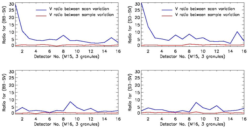
Figure 12.
Two way Analysis of Variance (ANOVA) test ratio versus 16 detectors for dBB ratio (left panels) and dSD ratio (right panels) along tracks and along scans in M15 (top panels) and M16 (bottom panels).
B. Noise Analysis Using Solar Diffuser Thermal Radiance from Operational Calibration Algorithm
The SDR radiometric calibration algorithms convert raw data from Earth View observations into SDR radiance, reflectance, and brightness temperature products. In the operational calibration algorithm, the SD radiance is calculated using the following equation (similar to the equation for earth view) for VIIRS [19,20]:
where is the band-averaged spectral radiance at the solar diffuser for scan angle . refers to Response Versus Scan function at scan angle for band B. Here we assume it to be one because there is no RVS Look-Up-Table for the SD (no prelaunch measurement) in thermal infrared band. is the spectral reflectance of RTA. is the Blackbody spectral radiance from Planck’s function. is jth order coefficient of the response function after calibration update.
F is the factor for radiance coefficient which is computed from:
where is the spectral emissivity of the BB. t is the start time of the acquisition period and the average counts per scan viewing the OBCBB is
The number of frames per scan is 48 for the “M” band.
In Equation (18); is the band-averaged OBCBB reflected radiance:
Where the factors , , and represent the fraction of the reflectance off the OBCBB originating from the sources blackbody shield, cavity, and telescope [19,20].
To compute the SD thermal radiance, several Look Up Tables (LUTs) were used. The BB, SD, and SV observations from VIIRS On-board Calibrator Intermediate Product (OBCIP) and telemetry measurements are retrieved to compute SD radiance in TEB spectral bands (VIIRS M15 and M16).
In Figure 13, top panel shows SD radiance computed from the operational calibration algorithm (Equation (20)) for HAM A versus scan number for two continuous granules (t0755175_e0756417 and t0756429_e0758071) on June 30, 2015, and the bottom panel shows the ratio of SD radiance between HAM sides A and B in M15. From top panel, we found that SD radiance increases from detector 1 to detector 16, and there is a trend that SD radiance keep changing with scan number (or time) for different portion of orbit, so a normal standard deviation method cannot be used to analyze SD radiance directly. To remove the impact of Response versus Scan angle (RVS), we will analyze the ratio of SD radiance between HAM sides A and B (). Bottom panel illustrates that the changing trend with time in different portion of the orbit is removed after using the ratio of SD radiance between HAM side A and B. Therefore, we can utilize the normal standard deviation method to evaluate the SD radiance ratio () directly.
The V ratios (defined in Equation (12)) computed from SD radiance ratio () are compared for 16 detectors in M15 and M16 (Figure 14). We found that V ratio between scans (blue lines) is much larger than that between samples (red lines) for both of M15 and M16, which means that the variation between scans is one of the major reasons for the striping observed in VIIRS imagery. This figure also shows the noise level versus detectors along the track direction: detectors 1 and 2 have much higher noise levels than other detectors in M15. In M16, detectors 9 and 12 have about twice and one half higher noise level than other detectors. Within the scan direction, the V ratio values for all detectors are very similar for either M15 or M16. Therefore, the detector noise due to along track variation has higher chance causing the striping observed in the images.
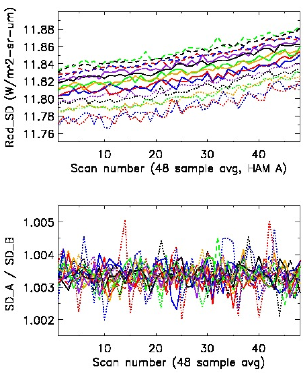
Figure 13.
Detector dependent SD radiance for Half Angle Mirror (HAM) side A (top) and ratio of SD radiance between HAM sides A and B (bottom) in M15 on 30 June 2015. Each line represents a detector. Note: use 48-sample averaged value for each scan.
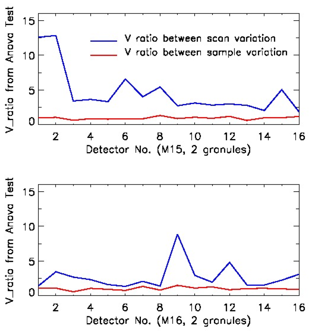
Figure 14.
V ratios (defined in Equation (16)) from ANOVA tests for SD radiance HAM side ratio for 16 detectors in M15 (top) and M16 (bottom) for two granules on 30 June 2015.
The cumulative histogram method discussed in Section 4.1 (Equations (7) and (8) can also be used for SD radiance to show detector-to-detector variation. The cumulative histogram of SD radiance for one granule d20130619_t0746 over the Bay of Bengal in M15 and M16 is provided in Figure 15. During this short period (about 1 min and 24 s), the effect of SD radiance changing over time should be small, so Figure 15 shows the cumulative histogram for SD radiance which is computed using the TEB operational calibration algorithm Equation (16). X-axis represents the SD radiance, and Y-axis is the percentage of the pixels with the value less than X-axis value. Each line is for one detector. The horizontal distance is approximately a constant. The maximum horizontal distance between Det 1 and Det 15 in M15 (left panel) and M16 (right panel) are 0.0655 and 0.050, respectively. Considering the radiance range, the relative magnitude (defined by Equation (8)) in M16 is 0.4036, which is larger than 0.3475 in M15. That means the detectors in M16 are more stable than those in M15, but the striping in M16 is more apparent. Comparing with EV striping analysis which was used for BT, the relative magnitude using onboard SD radiance is much larger and can show the detector-to-detector variation more clearly. On the other hand, since there is no thermistor on the SD, its temperature uniformity is not known so the analysis may be affected by any temperature trend on the SD surface.
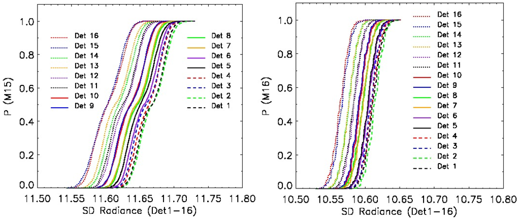
Figure 15.
The cumulative histogram for SD radiance () over the Bay of Bengal in M15 (left) and M16 (right) for granule d20130619_t0746 on 19 June 2013.
C. Correlation between dBB and dSD for Detector 1 in M15
One hypothesis is that the DCR and detector instability may have contributed to the striping. As a proof, the correlation between dBB (which is an indicator of DCR and detector noise short term) and dSD (which is proxy for earth view) is analyzed. DCR and detector noise can be propagated to the dSD as well as earth view data. Therefore, in addition to the above analysis, we have also studied the possible relationship between dBB and dSD for same cases as in Table 2. Since detector 1 in M15 is much more noisy than other detectors (see Figure 12 and Figure 14), the following study focuses on detector 1 in M15. dBB has no trend over the orbital time, so dBB variation is mostly due to random noise, detector and DCR instability. If there is correlation between dBB and dSD, then the DCR effect may be related to the striping in dSD. As an example, we use one granule (d20130619_t0748_e0749) OBCIP file in Bengal Case 1, which is about 1 min and 24 s. During this short period, we assume BB temperature does not change. Table 3 summarizes the linear correlation coefficients between dBB and dSD (in the 3rd column), as well as along track and along scan Allan deviation of SD Radiance in M15 and M16. In general, dBB and dSD are more correlated over the tropical region than polar region. We have also analyzed the ratio of along track to along scan Allan Deviation of solar diffuser radiance, which show larger values for tropical cases than polar cases.
Figure 16 uses one granule (d20130619_t0748_e0749) OBCIP file in Bengal Case 1 as an example, left panel shows the correlation between dBB and dSD, and the correlation coefficients is about 0.8345. Right panel shows the horizontal divergence or striping through the cumulative histogram of dBB. The maximum horizontal divergence among detectors for dBB and dSD are 181.985 and 129.953, respectively. Table 4 summarizes the linear correlation coefficients between dBB and dSD and the averaged horizontal divergence of dBB and dSD for six cases. In general, higher correlation corresponds to larger averaged horizontal divergence.
Table 3.
Correlation coefficients between dBB and dSD, as well as along track and along scan Allan deviation of solar diffuser radiance in M15 and M16.
| Cases | Granule | Coeff.* for det 1 in M15 | Allan Deviation for SD_Rad In M15 | Allan Deviation for SD_Rad In M16 | ||||
|---|---|---|---|---|---|---|---|---|
| Along Track | Along Scan | Ratio | Along Track | Along Scan | Ratio | |||
| Bengal: case1 | d20130619_t0746444 | 0.8345 | 0.00919 | 0.00479 | 1.91827 | 0.00709 | 0.00442 | 1.60429 |
| Bengal: case2 | d20140622_t0753301 | 0.8151 | 0.00920 | 0.00486 | 1.89414 | 0.00714 | 0.00449 | 1.59022 |
| Bengal: case3 | d20140703_t0748470 | 0.7912 | 0.00901 | 0.00479 | 1.88105 | 0.00704 | 0.00443 | 1.58842 |
| Alaska: case 1 | d20140520_t2158272 | 0.5981 | 0.00827 | 0.00483 | 1.71272 | 0.00652 | 0.00443 | 1.47338 |
| Alaska: case 2 | d20140603_t2237573 | 0.4225 | 0.00842 | 0.00479 | 1.75669 | 0.00647 | 0.00439 | 1.47115 |
| Polar: case 3 | d20150421_t1802552 | 0.011 | 0.00793 | 0.00484 | 1.63808 | 0.00585 | 0.00441 | 1.32739 |
Coeff * refers to the correlation coefficient.
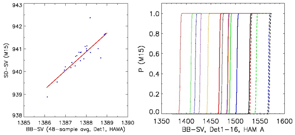
Figure 16.
Linear correlation between dBB and dSD (left) and the cumulative histogram of 48-sample averaged dBB (right) for detector 1 in HAM side A and band M15 over a granule of the Bay of Bengal in case1.
Table 4.
Correlation coefficients between dBB and dSD, as well as the maximum horizontal distance from dBB and dSD in M15.
| Cases | Granule | Correlation Coefficients for Det 1 in M15 | dBB Range | dSD Range |
|---|---|---|---|---|
| Bengal: case 1 | d20130619_t0746444 | 0.8345 | 181.985 | 129.953 |
| Bengal: case 2 | d20140622_t0753301 | 0.8151 | 179.776 | 130.252 |
| Bengal: case 3 | d20140703_t0748470 | 0.7912 | 179.952 | 130.475 |
| Alaska: case 1 | d20140520_t2158272 | 0.5981 | 180.691 | 129.168 |
| Alaska: case 2 | d20140603_t2237573 | 0.4225 | 181.486 | 129.872 |
| Polar: case 3 | d20150421_t1802552 | 0.011 | 179.917 | 124.966 |
5. Conclusions
In this study, we have investigated the striping pattern in VIIRS SST imagery using LBLRTM simulation and VIIRS SDR observation data. The analysis indicates that the striping is likely related to the difference in detector level RSR. The results from LBLRTM show that BT difference between the band averaged and detector level RSR has some atmospheric dependency, i.e., the difference over tropical region is larger than that over polar region. The magnitude of the difference between tropical and subarctic summer is 0.017 K in M15 − M16, 0.04 K in M16, and −0.019 K in M15. Results also show that band M16 is more sensitive to the atmospheric conditions due to higher water vapor absorption. M15 − M16 is the critical quantity in SST retrieval, which shows more apparent striping than single bands because of smaller signal-to-noise ratio. Detector # 1–3 shows large atmospheric effect in M15 − M16 and M16. With the band average as reference, detector # 1 has the largest deviation (0.055 K) for tropical case, which is close to 0.05 K in previous study using MODTRAN[4].
In addition to the model simulation analysis, we have also performed case studies to analyze the striping in VIIRS SDR brightness temperature observation data over tropical and polar region. Three different methods including cumulative histogram, standard deviation, and Allan deviation methods, are utilized to quantify the striping in the images of VIIRS earth view data (BT) for bands M15, M16, and M15 − M16. Results show that the histogram divergence difference between tropical and polar region is 0.040 K in, 0.053 K in M16, and 0.003 K in M15 respectively. They are all slightly higher than those from model output. In general, VIIRS SDR brightness temperature observation has larger variability when compared with the model output. However, difference due to atmospheric condition is small in an absolute value, but it also plays a role in causing the striping.
The Earth View data is complex because the noise is mixed with diverse signals. The onboard calibration data excludes the atmospheric effect and is spatially uniform, so it is used to analyze the instrument effect (such as fixed pattern noise) which is a possible factor affecting the striping pattern. The thermal band detector noise characterization has been studied using the raw data of BB, SD, and SV. The SD radiance is also computed from the operational TEB calibration algorithm, which has an advantage because it acts as a proxy of SST and can simulate the impact of SST. ANOVA tests of dBB, dSD, and SD radiance demonstrate that the noise along track direction is the major reason for the striping observed in VIIRS imagery. In along track direction, detectors 1 and 2 in M15 show higher noise levels than other detectors, detectors 9 and 12 in M16 also have much higher noise level than other detectors. Within the scan direction, the ratio (defined by Equation (16)) in ANOVA test for all detectors are very similar for either M15 or M16. Since the dBB has no trend with time, its variation is mostly from random noise, detector instability and DCR short term. The results show that the variation of dBB with scan in along track direction, i.e., detector instability and DCR short term, are the dominant factor for dBB variation. We also found evidence of correlation between dSD and dBB for a detector 1 in M15. Since PRT in dBB is stable during the short period, the DCR instability is likely related to the striping in dSD and earth view data. On the other hand, further analysis is needed with more data samples. These findings will help us better understand the impact of the difference in detector level RSR and noise on VIIRS geophysical retrieval which can also potentially lead to further SDR processing improvements.
Acknowledgments
The authors would like to thank the anonymous reviewers for their constructive comments and suggestions which helped us improve the clarity of the manuscript. We also thank the VIIRS SDR team members in general, and Boryana Efremova and David Moyer, in particular, for fruitful discussions during the team telecons on the root cause of the striping. We also appreciate the help from Zhenping Li for help with the histogram based striping characterization. Thanks are extended to Slawomir Blonski, Wenhui Wang, Bin Zhang, Yan Bai, and Jason Choi for their help in the data processing and analysis. The views, opinions, and findings contained in this paper are those of the authors and should not be construed as official positions, policy, or decisions of the NOAA or the U. S. Government.
Author Contributions
Zhuo Wang contributed to the design of the study, the development of methodology and software code, performed the analysis and wrote the manuscript. Changyong Cao contributed to the design of the study, the development of methodology, and provided technical oversight of the project.
Conflicts of Interest
The authors declare no conflict of interest.
References
- Miller, S.D.; Lee, T.F.; Fennimore, R.L. Satellite-based imagery techniques for daytime cloud/snow delineation from MODIS. J. Appl. Meteor. 2005, 44, 987–997. [Google Scholar] [CrossRef]
- Bouali, M.; Ignatov, A. Adaptive reduction of striping for improved sea surface temperature imagery from Suomi National Polar Orbiting Partnership (S-NPP) Visible Infrared Imaging Radiometer Suite (VIIRS). J. Atmos. Ocean. Technol. 2014, 31, 150–163. [Google Scholar] [CrossRef]
- Padula, F.; Cao, C. Preliminary study of the Suomi NPP VIIRS detector-level spectral response function effects for the long-wave infrared bands M15 and M16. Proc. SPIE 2014. [Google Scholar] [CrossRef]
- Padula, F.; Cao, C. Detector-level spectral characterization of the Suomi NPP VIIRS long-wave infrared bands M15 & M16. Appl. Opt. 2015, 54, 5109–5116. [Google Scholar] [PubMed]
- Godin, R. VIIRS Sea Surface Temperature Algorithm Theoretical Basis Document (ATBD); Goddard Space Flight Center Greenbelt: Greenbelt, MD, USA, 2013. [Google Scholar]
- Liou, K.N. An Introduction to Atmospheric Radiation, 2nd ed.; International Geophysics Series; Academic Press: San Deigo, CA, USA, 2002; Volume 84. [Google Scholar]
- Berk, A.; Anderson, G.P.; Acharya, P.K.; Shettle, E.P. MODTRAN 5.2.1 User’s Manual; Space Vehicles Directorate: Hanscom AFB, MA, USA, 2011. [Google Scholar]
- Clough, S.A.; Iacono, M.J.; Moncet, J.-L. Line-by-line calculation of atmospheric fluxes and cooling rates: Application to water vapor. J. Geophys. Res. 1992, 97, 15761–15785. [Google Scholar] [CrossRef]
- Clough, S.A.; Shephard, M.W.; Mlawer, E.J.; Delamere, J.S.; Iacono, M.J.; Cady-Pereira, K.; Boukabara, S.; Brown, P.D. Atmospheric radiative transfer modeling: A summary of the AER codes. J. Quant. Spectrosc. Radiat. Transf. 2005, 91, 233–244. [Google Scholar] [CrossRef]
- Alvarado, M.J.; Payne, V.H.; Mlawer, E.J.; Uymin, G.; Shephard, M.W.; Cady-Pereira, K.E.; Delamere, J.S.; Moncetm, J.L. Performance of the Line-By-Line Radiative Transfer Model (LBLRTM) for temperature, water vapor, and trace gas retrievals: Recent updates evaluated with IASI case studies. Atmos. Chem. Phys. 2013, 13, 6687–6711. [Google Scholar] [CrossRef]
- Moncet, J.L.; Uymin, G.; Lipton, A.E.; Snell, H.E. Infrared radiance modeling by optimal spectral sampling. J. Atmos. Sci. 2008, 65, 3917–3934. [Google Scholar] [CrossRef]
- Rothman, L.S.; Gordon, I.E.; Barbe, A.; Benner, D.C.; Bernath, P.F.; Birk, M.; Boudon, V.; Brown, L.R.; Campargue, A.; Champion, J.-P.; et al. The HITRAN 2008 molecular spectroscopic database. J. Quant. Spectrosc. Radiat. Transf. 2009, 110, 533–572. [Google Scholar] [CrossRef]
- Rosenkranz, P.W. Shape of the 5 mm oxygen band in the atmosphere. IEEE Trans. Antennas Propag. 1975, 23, 498–506. [Google Scholar] [CrossRef]
- Mlawer, E.J.; Payne, V.H.; Moncet, J.-L.; Delamere, J.S.; Alvarado, M.J.; Tobin, D.D. Development and recent evaluation of the MK_CKD model of continuum absorption. Philos. Trans. R. Soc. 2012, 370, 2520–2556. [Google Scholar] [CrossRef] [PubMed]
- Martin, S. An Introduction to Ocean Remote Sensing; Cambridge University Press: Cambridge, UK, 2004. [Google Scholar]
- Weinreb, M.P.; Xie, R.R.; Lienesch, J.H.; Crosby, D.S. Destriping GOES images by matching empirical distribution functions. Remote Sens. Environ. 1989, 29, 185–195. [Google Scholar] [CrossRef]
- Li, Z.; Yu, F. A Real Time De-Striping Algorithm for Geostationary Operational Environmental Satellite (GOES) 15 Sounder Images. Available online: http://digitalcommons.usu.edu/cgi/viewcontent.cgi?filename=0&article=1197&context=calcon&type=additional (accessed on 6 February 2016).
- Allan, D.W.; Ashby, N.; Hodge, C.C. Appendix A: Time and frequency measures accuracy, error, precision, predictability, stability, and uncertainty. In The Science of Timekeeping; Hewlett Packard Application Note 1289; Hewlett-Packard Company: Englewood, CO, USA, 1997; pp. 56–65. [Google Scholar]
- Cao, C.; Xiong, X.; Wolfe, R.; De Luccia, F.; Liu, Q.; Blonski, S.; Lin, G.; Nishihama, M.; Pogorzala, D.; Oudrari, H. Visible Infrared Imaging Radiometer Suite (VIIRS) Sensor Data Record (SDR) User’s Guide, version 1.2; National Oceanic and Atmospheric Administration, National Environmental Satellite, Data, and Information Service: Washington, DC, USA, September 2013. [Google Scholar]
- Baker, N.; Kilcoyne, H.; NOAA. Joint Polar Satellite System (JPSS) VIIRS Radiometric Calibration Algorithm Theoretical Basis Document. Available online: http://npp.gsfc.nasa.gov/sciencedocs/2015-06/474-00027_ATBD-VIIRS-Radiometric-Calibration_C.pdf (accessed on 6 February 2016).
© 2016 by the authors; licensee MDPI, Basel, Switzerland. This article is an open access article distributed under the terms and conditions of the Creative Commons by Attribution (CC-BY) license (http://creativecommons.org/licenses/by/4.0/).