Validation of a Forage Production Index (FPI) Derived from MODIS fCover Time-Series Using High-Resolution Satellite Imagery: Methodology, Results and Opportunities

Abstract

An index-based insurance solution was developed to estimate and monitor near real-time forage production using the indicator Forage Production Index (FPI) as a surrogate of the grassland production. The FPI corresponds to the integral of the fraction of green vegetation cover derived from moderate spatial resolution time series images and was calculated at the 6 km × 6 km scale. An upscaled approach based on direct validation was used that compared FPI with field-collected biomass data and high spatial resolution (HR) time series images. The experimental site was located in the Lot and Aveyron departments of southwestern France. Data collected included biomass ground measurements from grassland plots at 28 farms for the years 2012, 2013 and 2014 and HR images covering the Lot department in 2013 (n = 26) and 2014 (n = 22). Direct comparison with ground-measured yield led to good accuracy (R² = 0.71 and RMSE = 14.5%). With indirect comparison, the relationship was still strong (R² ranging from 0.78 to 0.93) and informative. These results highlight the effect of disaggregation, the grassland sampling rate, and irregularity of image acquisition in the HR time series. In advance of Sentinel-2, this study provides valuable information on the strengths and weaknesses of a potential index-based insurance product from HR time series images.

1. Introduction

Grasslands are one of the largest ecosystems in the world, covering 52.5 million km² or 40.5% of terrestrial area excluding Greenland and Antarctica. In many countries, they are crucial for supporting livestock activities [1]. However, grasslands are very sensitive to climatic events [2,3], with drought representing a major peril faced by hay producers. Depending on the amount and timing of rainfall, the quantity and quality of hay can change significantly [4,5]. To mitigate drought impacts, producers use auto-insurance solutions. It consists in the modification of the production system strategy such as increasing hay stocks, converting grain crop into forage or advance selling of animals [6]. They can also request indemnification through private or public insurances. For forage, traditional insurance systems used for cereals, oil and protein crops, vegetables, vineyards, fruit and maize silage are not applicable for three major reasons. First, grassland production is not easily measurable. The grassland management system may vary significantly from one farm to another and according to annual weather conditions. Second, grasslands can be harvested several times a year and/or are grazed. Finally, the forage produced is usually consumed by animals (around 90% of total production). This information does not appear in farm accounts and a historical reference of production does not exist. Because of these reasons, accurate loss estimates are difficult to achieve even when relying on costly and time-consuming human assessment. To overcome these difficulties, index-based insurance (IBI) was developed [7]. Unlike traditional insurance schemes that assess losses on an individual basis, IBI offers payouts based on an external indicator, or index, which triggers a payment to all insured farmers within a geographically defined space [8,9]. Different types of IBI exist and are differentiated by the data used to derive the index, such as a weather-based, yield-based and satellite-based index [10,11,12]. For the latter, an index correlated with production is computed from satellite imagery. The information provided by remote sensing is about “rainfall” [13] or “vegetation estimates” [14,15]. For “vegetation estimates,” two types of remote sensing-derived indices are currently used (or under consideration) and are often produced with moderate resolution (MR) remote sensing products: vegetation index [16,17,18] and biophysical variable [19,20].

Satellite-derived products and information should be validated, particularly if they are used for policy making, fiscal scrutiny, or indemnities [21]. To guarantee that the insurance product used to indemnify farmers is based on forage losses closest to that which could be measured in the field, a validation of the remote sensing information produced (including estimates of uncertainties) is mandatory. Remote sensing product validation is “the process of assessing by independent means the accuracy of data products derived from the system outputs” [22].

The validation of MR remote sensing time series products is particularly challenging because of the (1) limited availability of adequate and independent reference data; (2) variability in situation and sources of errors at a national or global scale; and (3) mismatches between the spatial definition of ground observations used as independent data of the target variable and MR pixel size. Together, these factors contribute to difficulties in accuracy assessment and higher levels of uncertainty.

Available methodologies highlight two possible approaches for validation. Both help assess accuracy of the target variable with the same measure on the ground distributed over appropriate sampling schemes. In the first approach, called direct validation, two techniques can be distinguished according to the reference data used. Direct comparison is based on field data measurements [23]. Given that ground data collection is time consuming and expensive, field measurement is often limited in time and space and, consequently, not representative of multiple conditions [24]. Another limitation is that the compared target variable may be observed using different data collection methods (e.g., remote sensing sensors and ground measurements device). In contrast, indirect comparison uses high resolution (HR) images that are later aggregated to the scale of MR products [25,26]. This technique helps to overcome the time-space ground data limitation. Using HR images as an intermediate scale of measurement improves spatial coverage but requires an upscaling step that introduces new problems related to sampling strategy [27] and the processing of HR time series with irregular image acquisition frequencies [21].

An alternative to direct validation is indirect validation [28,29]. This approach consists of benchmarking similar remote sensing products for one target variable via intercomparison. Working at the same spatial scale avoids the issue of sampling strategy and the potential use of a large dataset improves the ability to cover a wide range of pedoclimatic conditions and to better estimate uncertainties. However, results from indirect validation cannot be considered an assessment of accuracy as in direct validation approaches because this approach does not involve true reference data. While some consensus now exists on methods to validate MR products [30], new types of HR time series are now available or are forthcoming (e.g., Landsat 8 combined with Sentinel-2 data) and this domain of research remains very active [21].

In France, grasslands cover 44% of arable land, or 12.8 million ha [31], and are a key element for livestock production. When drought occurs, farmers are indemnified by the French Ministry of Agriculture. Losses are estimated by the Ministry’s Statistics Department with information provided by growers’ associations and other collecting agencies. Since 2010, the French state has gradually transferred risk coverage to the private sector to realize savings [32,33].

In that context, Crédit Agricole Assurances Pacifica, associated with Airbus Defence and Space (D&S), proposed in 2016 an index-based insurance solution which could assess local forage production [34,35,36]. They developed an indicator called Forage Production Index (FPI) to estimate and monitor in near real-time the forage abundance in France. This insurance product will be offered to farmers to offset losses from drought and other extreme meteorological events. Processing is fully automatic and is based on the biophysical parameter fraction of green vegetation cover (fCover) obtained from MODIS time series images (at 250 m spatial resolution).

In a previous study [37], a direct comparison between in situ grassland biomass measurements and FPI derived from fCover measured with HR time series was conducted. Ground data for validation were collected with a motorized mower and weighed before and after drying to calculate dry matter production of each sample area. Results indicated that fCover was an appropriate proxy for grassland biomass production [37]. The fraction of photosynthetically active radiation absorbed by the canopy (fAPAR) was also analyzed and replaced fCover in the FPI equation [19]. fAPAR depends on canopy structure and illumination conditions [38] and is a very useful input for a number of primary productivity models based on simple light use efficiency considerations [39]. This past research showed that the correlation between biomass and the FPI is good when using either fAPAR or fCover. However, even though the results are promising, a need still exists to validate FPI at the spatial scale of the insurance product.

The objective of this paper is to present an accuracy assessment methodology for the Forage Production Index derived from MODIS fCover time series. FPI calculation is discussed followed by validation of FPI using a direct approach that integrates direct and indirect comparison techniques as recommended by [24,26,29,40]. The methodology was inspired from one developed by the Land Product Validation sub-group of the Committee for Earth Observation Satellites (CEOS) who established best practices and guidelines under which validation of MR products should be made [26]. It offers opportunities for testing the potential of HR spatial and temporal time series images from platforms such as Landsat 8 and Sentinel-2 to improve measures of forage production losses compared to MR time series.

2. Forage Production Index (FPI) Processing Methodology

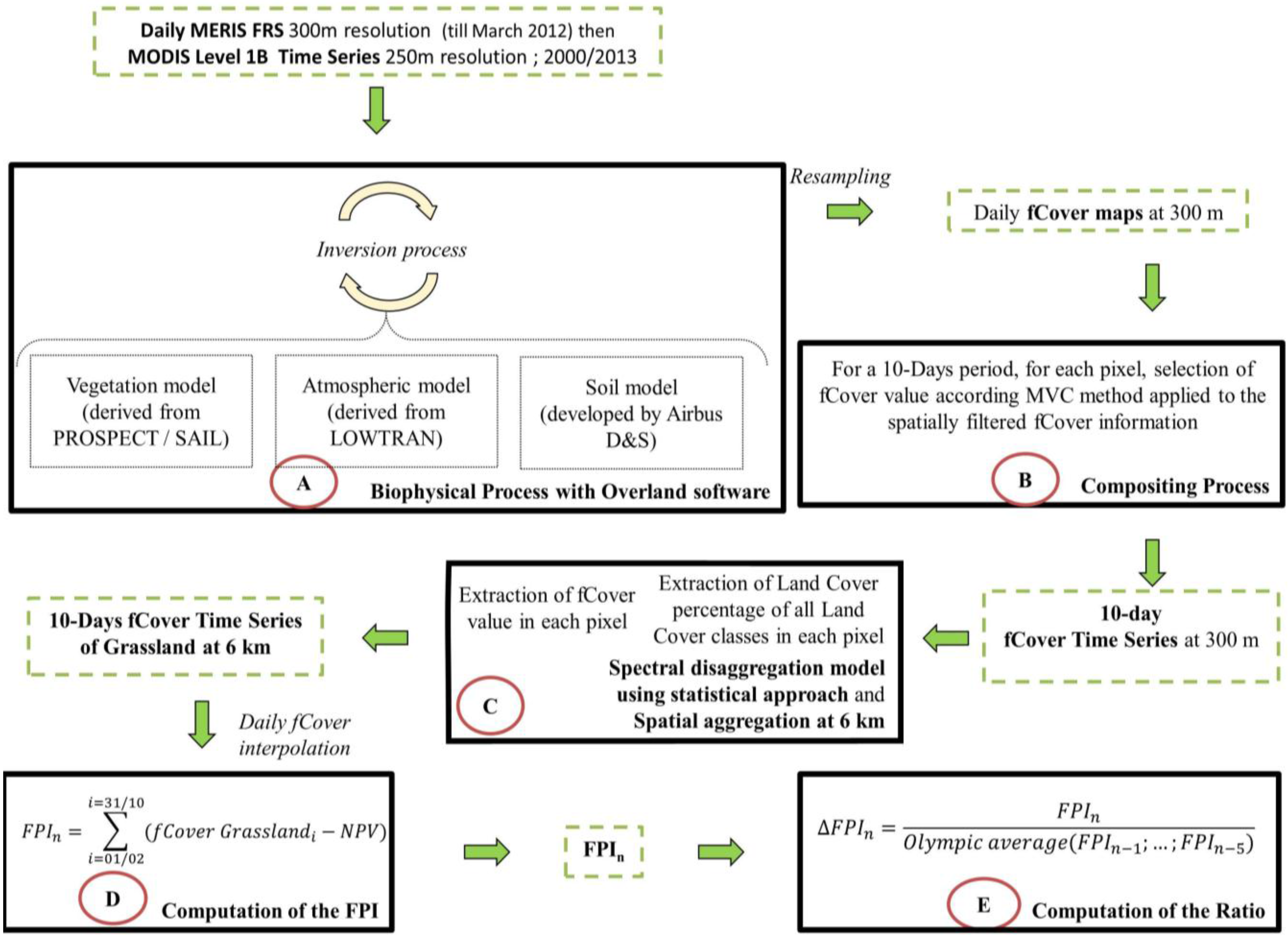
The FPI processing chain is a fully automatic process (Figure 1). Biophysical parameters, in particular fCover and fAPAR, were calculated using the Overland image processing software developed by Airbus Defence and Space. This tool extracts vegetation parameters by inverting a radiative transfer model that couples scene and atmospheric models [41]. Overland integrates most recently developed models [42] (Figure 1A), Low Resolution Transmission (LOWTRAN) [43] for the atmospheric component, a model of leaf optical Properties Spectra (PROSPECT) [44] and Scattering by Arbitrarily Inclined Leaves (SAIL) [45] for the vegetation component. The vegetation model has been upgraded by adding a “brown” contribution (for non-productive vegetation) to the foliage. A uniform canopy model would consider a homogeneous mixture of green and brown leaves, characterized by separate PROSPECT variable descriptions. Because vegetation in one MR pixel is likely heterogeneous, a dedicated composite canopy model was designed that adds separate contributions from green and bare, or senescent, plots. The overall model is full Bidirectional Reflectance Distribution Function (BRDF) and takes into account the sensor viewing and sun illumination directions, though fCover is ultimately computed in a normalized vertical direction. The fCover produced from MR products with this processing chain was previously validated in the Geoland project [41]. Soil reflectance is a needed input to the overall model and is obtained once by capturing a spectral signature of local soils from one satellite image. However, this reflectance is allowed to vary locally both in time and space depending on wetness and roughness of the soil surface.

Figure 1. The processing chain of the Forage Production Index (FPI). Rectangles in black bold illustrate the main step of the processing chain. Green dotted rectangles are the intermediate products. PROSPECT = Properties Spectra; SAILn = Scattering by Arbitrarily Inclined Leaves; LOWTRAN = Low Resolution Transmission; D&S = & Space; MVC = Maximum Value Composite; NPV = Non-Productive Vegetation; fCover = Fraction of Green Cover.

Figure 1. The processing chain of the Forage Production Index (FPI). Rectangles in black bold illustrate the main step of the processing chain. Green dotted rectangles are the intermediate products. PROSPECT = Properties Spectra; SAILn = Scattering by Arbitrarily Inclined Leaves; LOWTRAN = Low Resolution Transmission; D&S = & Space; MVC = Maximum Value Composite; NPV = Non-Productive Vegetation; fCover = Fraction of Green Cover.

Model inversion was achieved by minimizing a cost function using an optimization technique with a Gauss-Newton iterative procedure. A parameter, called “Fit”, is produced that defines the quality of the inversion process by measuring the difference between estimated and observed reflectance values. Lowest values correspond to situations where vegetation cover characteristics are well modeled. In addition to the biophysical processing, clouds are automatically masked in each image. A compositing algorithm then generates seamless 10-day maps of major vegetation parameters, including fCover. For each pixel, fCover in a 10-day period was selected according to the Maximum Value Composite method [46] applied to the spatially filtered fCover information of each observation (Figure 1B).

Because one MR pixel may contain different land cover types, a disaggregation method based on a statistical approach originally applied to reflectances [47,48] was used to determine fCover values for grassland (Figure 1C). This method estimates fCover values for each land cover class from the input of fCover estimates for a population and the a priori knowledge of each land cover class’s contribution to each pixel (local aspect). Consequently, fCover was calculated at an Elementary Statistical Unit (ESU) scale of 6 km × 6 km. The land cover database used for disaggregation was provided by farmer declarations in the 2012 Common Agricultural Policy (RPG Anonyme ASP 2012) and completed with the Corine Land Cover Database 2006 (European Environment Agency, 2012). Surfaces of each land cover in the ESU are combined and form the final land cover database. The grassland class contains natural (native or sown six years or more) and temporal (sown less than six years with a minimum of 20% Poaceae) grassland, but does not include artificial grassland (sown less than six years with a minimum of 80% Fabaceae).

The 10-day ESU fCover values were then interpolated to daily fCover with the moving average method allowing for a daily profile to be extracted for each ESU. The FPI was derived from the fCover integral and used as a surrogate for forage production for a given period of time (Equation (1)).

$$FP{I}_n={\displaystyle \sum }_{i=01/02}^{i=31/10}\left(fCoverGrasslan{d}_i-NPV\right)$$

(1)

The FPI was calculated for a year n and is the sum of daily fCover grassland between February 1st and October 31st (fCover Grassland_i) from which the part characterizing the proportion of Non-Productive Vegetation (NPV) is subtracted (Figure 1D). This parameter corresponds to biomass that could not be harvested. It is an empirical value, fixed in time and variable across space, based on statistical grassland yield data provided by the French Ministry of Agriculture at department scale. The variation in biomass production is defined as a ratio between the annual FPI and the historical average FPI. In the insurance product, payouts are indexed based on the ratio between annual FPI and the Olympic average of FPI (ΔFPI_n) of the last five years (Equation (2); Figure 1E).

$$\Delta FP{I}_n=\frac{FP{I}_n}{Olympic average\left(FP{I}_{n-1};\dots ;FP{I}_{n-5}\right)}$$

(2)

This averaging method excludes both the highest and lowest observations from a sample before calculating the average and is a common strategy in agricultural insurance schemes to calculate reference production levels [49].

The required inputs for the processing chain are two MODIS/Terra products: Calibrated radiances with five bands (between 0.45 and 2.20 µm) L1B at 500 m spatial resolution (MOD02HKM) and calibrated radiances with two bands (between 0.62 and 0.88 µm) L1B at 250 m spatial resolution (MOD02QKM).

Geometric corrections for the images were applied using the auxiliary file containing geolocation fields L1A at 1 km spatial resolution (MOD03) with the MODIS Reprojection Tool Swath (MRTSwath deployed by the Land Processes Distributed Active Archive Center) [50].

Biophysical processing was then conducted on the two bands at 250 m (bands 1 and 2) and the five bands at 500 m (bands 3 to 7). Finally, daily fCover were produced at a 300 m spatial resolution in order to be similar to, and compatible with, previous products generated from MERIS data prior to the loss of the Envisat satellite in March 2012.

3. Direct Comparison of Field Measurements and MR Product

Direct comparison focused on analyzing the accuracy of information used in the insurance product to calculate the payouts. It consisted of evaluating the performance of the ratio of annual biomass variation and baseline values derived from MR fCover grassland time series by comparing it to ones obtained with field measurements.

3.1. Study Site

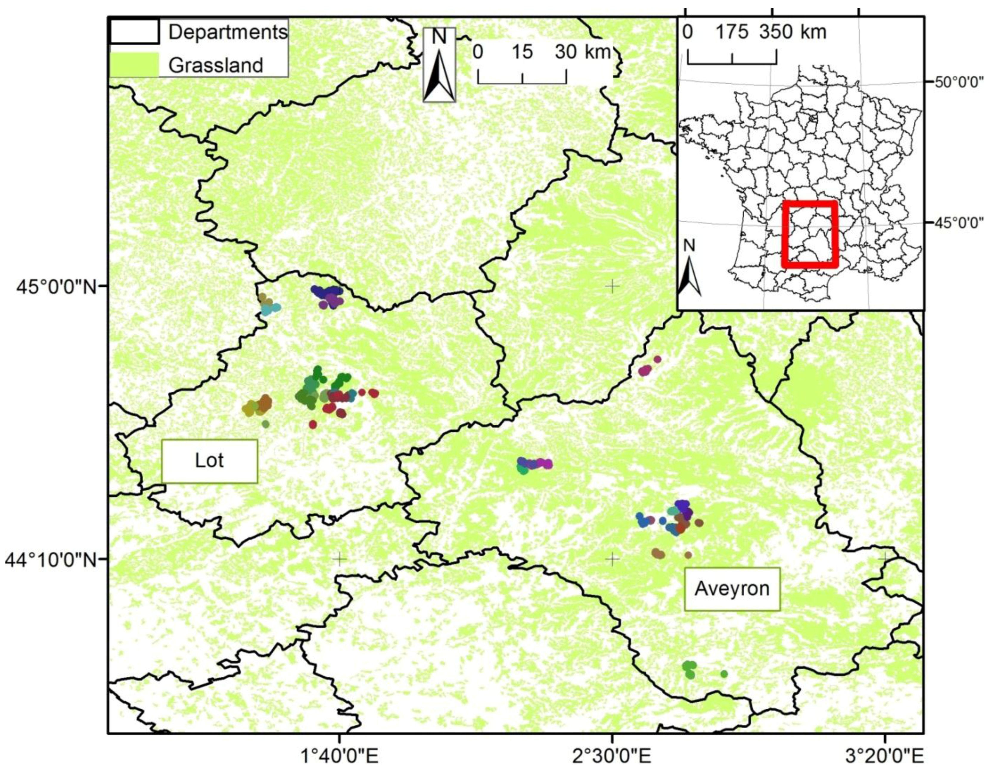
The study site was located in the Lot and Aveyron departments of southwestern France (Figure 2). Agricultural lands in this area are dominated by grassland and pasture used mainly for breeding sheep and cattle [51] (90% in Aveyron and 66% in Lot). The period for direct comparison of the FPI was 2012–2014, beginning in February and ending (for each ESU) according to farmers’ practice and grassland production.

Figure 2. Sampling sites in the Lot and Aveyron departments. Colored dots represent the grassland plot sampled with each color representing one of 28 participating farms.

Figure 2. Sampling sites in the Lot and Aveyron departments. Colored dots represent the grassland plot sampled with each color representing one of 28 participating farms.

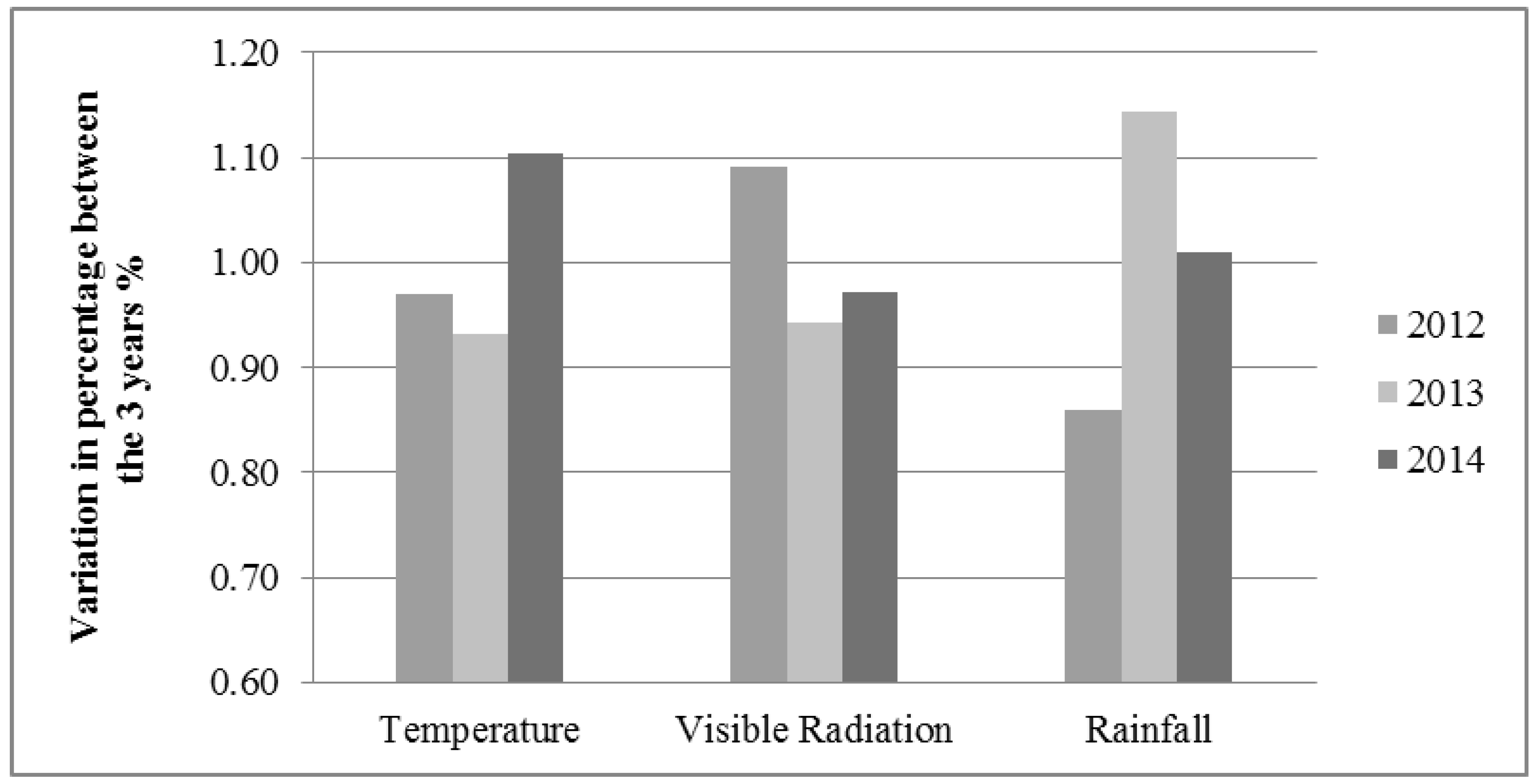
Figure 3 shows variation in three main meteorological parameters (temperature, visible radiation (electromagnetic radiation with wavelengths between 380 and 780 nanometers), and rainfall) associated with grassland production. Variations were calculated by dividing the annual value of a given year by the average annual values of the other two years. Each parameter was summed from 1 February to 31 July [52]. This period is forced because of data non-availability after 31 July 2014. This is not really an issue because biomass produced in the first part of the year is the most important for breeders. It provides forage of high nutrient quality and in quantities sufficient to provide approximately 65% of annual needs [53]. Second, if cutting spring grass for hay stock is a common strategy within the study area, grassland management in summer and fall would be quite variable (e.g., it could be cut or grazed). Spring, then, is the main season when biomass production data could be consistently collected each year according to our protocol requirements (see Section 3.2).

The year 2012 had a water deficit of 10% compared to 2013 and 2014 and a high level of visible radiation, based on the percentage of variation of the averaged sum of rainfall and visible radiation within the study area. For 2013 and 2014, though cumulative rainfall and temperature are slightly different (2014: 1.01% and 1.10%; 2013: 1.14% and 0.93%, respectively, for cumulated rainfall and temperature), generally wet conditions resulted in a similar level of biomass production in the study area.

Figure 3. Variation in percentage of the averaged sum of temperature (°C), visible radiation (J·cm⁻¹) and rainfall (mm) from February 1 to July 31 in the defined ESU of the study area. Values were calculated by the value of a given year divided by the average of the other two years for each parameter.

Figure 3. Variation in percentage of the averaged sum of temperature (°C), visible radiation (J·cm⁻¹) and rainfall (mm) from February 1 to July 31 in the defined ESU of the study area. Values were calculated by the value of a given year divided by the average of the other two years for each parameter.

3.2. Method

Biomass production measurements during 2012, 2013 and 2014 were collected from 28 farms (Figure 2). The complete dataset contained 290 (679 ha), 768 (1739 ha) and 557 (1203 ha) natural and temporary grassland plots in 2012, 2013, and 2014, respectively. Yields (in tons of dry matter per hectare) for each plot were estimated by multiplying the total number of harvested hay bales by the average plot-specific bale yield. To obtain the latter estimate, measurements of weight and moisture were taken with a pallet scale and portable moisture meter from approximately 5% of the bales harvested in each plot (Figure 4A). Because grasslands have several growing cycles in a year, the annual biomass estimation of the plot corresponds to the sum of the yield after each mowing.

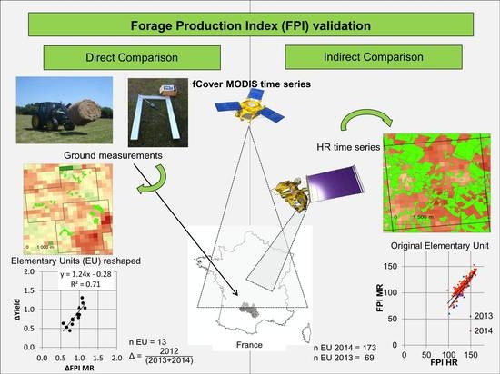
Figure 4. Workflow of the direct comparison methodology. fCover = fraction of green vegetation cover; MODIS = Moderate Resolution Imaging Spectroradiometer; MR = Moderate Resolution; FPI = Forage Production Index.

Figure 4. Workflow of the direct comparison methodology. fCover = fraction of green vegetation cover; MODIS = Moderate Resolution Imaging Spectroradiometer; MR = Moderate Resolution; FPI = Forage Production Index.

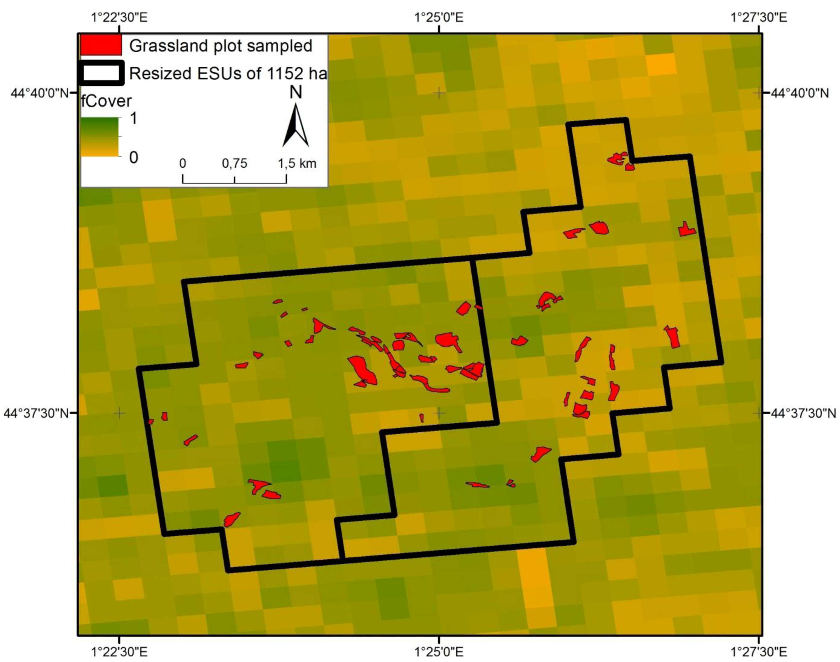
The difficulty of acquiring ground data over large areas and the need to create a representative grassland sample required resizing the original ESU (e.g., 6 km × 6 km) (Figure 4B). In each area where plot data were collected, ESU areas were downscaled from 3600 ha to 1152 ha. This spatial scale of 1152 ha is the best compromise between a high number of ESUs analyzed, a good sampling rate, and consistency with the initial size of 3600 ha. Resized ESUs, each of which represents 1152 ha, were delineated in the MODIS fCover layer based on the distribution of the sample plots (Figure 5). As a consequence, the percentage of grassland sampled increased from 2% for the original ESU of 3600 ha to 13.4% for the resized ESU of 1152 ha. Modifying the ESUs was expected to improve the accuracy of plot-level biomass production estimates by reducing the Root Mean Square Error (RMSE). A total of 13 ESUs of 1152 ha were analyzed.

Figure 5. Examples of two resized ESUs containing sampled grassland plots and designed for FPI direct comparison. The background image is a 10-day MODIS fCover image from 11 February 2012 to 20 February 2012 at a spatial resolution of 300 m.

Figure 5. Examples of two resized ESUs containing sampled grassland plots and designed for FPI direct comparison. The background image is a 10-day MODIS fCover image from 11 February 2012 to 20 February 2012 at a spatial resolution of 300 m.

For each of the 13 ESUs analyzed, a Yield_n index was computed using Equation (3) where YieldPlot_i is the annual biomass estimation of plot i and Surface_i the plot area. The Yield_n index was the annual ESU n biomass estimate in tons of dry matter per hectare that was compared with estimates obtained from the MR product.

$$Yiel{d}_n=\frac{{{\displaystyle \sum }}_{i=1}^j(YieldPlo{t}_i\times Surfac{e}_i)}{{{\displaystyle \sum }}_{i=1}^j(Surfac{e}_i)}$$

(3)

Each year, the ESU biomass production was computed from February 1 to the last harvest in the ESU (information collected during field campaign). FPI_MR was obtained with MODIS fCover grassland time series (Equation (1)) and Yield_n was computed with Equation (3) using field measurements. In the case of the FPI_MR, the proportion of non-productive vegetation (NPV) is not subtracted.

Next, the biomass production variation index (ΔFPI_MR or ΔYield depending on the data source) corresponding to the ratio of biomass produced for a given year divided by a baseline value (Equations (4) and (5)) was computed (Figure 4C). Because 2013 and 2014 are similar weather years and significantly different from 2012, the average of 2013 and 2014 biomass production is defined as the reference (or baseline) and 2012 is the year for which the variation of biomass production was analyzed.

$$Yiel{d}_n=\frac{{{\displaystyle \sum }}_{i=1}^j(YieldPlo{t}_i\times Surfac{e}_i)}{{{\displaystyle \sum }}_{i=1}^j(Surfac{e}_i)}$$

(4)

$$\Delta Yield=\frac{Yiel{d}_{2012}}{Mean\left(Yiel{d}_{2013};Yiel{d}_{2014}\right)}$$

(5)

The relationship between indices was quantified using RMSE and the coefficient of determination (R²) was assumed to be a good indicator of model fit. The RMSE obtained with a three-fold cross-validation method (RMSE_Pred) was also analyzed and allowed the models to be classified. Cross-validation gives an accurate measure of prediction capabilities [54]. The higher the RMSE_Pred, the greater overfitting of the model [55].

3.3. Results and Discussion

Figure 6 presents the relationship between ΔFPI_MR and ΔYield. The R² is 0.71 and indicates a good overall relationship between the indices. The ranges of biomass production variation indices were quite similar: 0.51 for ΔFPI_MR (from 0.56 to 1.07) and 0.88 for ΔYield (from 0.44 to 1.32). In 12 of the 13 ESUs (illustrated by dots in Figure 6), ΔFPI_MR varies in the same way as ΔYield meaning that variations in production were detected similarly. One ESU (symbolized by a triangle on Figure 6) highlights the single instance where the indices varied in opposite directions. The ratios obtained with field measurements (ΔYield) indicates a higher biomass production in 2012 compared to the reference value, whereas the ratio from the MR product shows a loss of biomass production (ΔFPI_MR = 0.99; ΔYield = 1.06). The difference between these values is small and does not represent a significant mismatch of the index variation. Overall, the relationship between ΔFPI_MR and ΔYield supports FPI derived from MR products as a suitable index to monitor variations in annual biomass production.

Figure 6. Scatterplot of the linear regression between ΔFPI_MR and ΔYield measured at 13 resized ESUs of 1152 ha for the period 2012–2014 in the Lot and Aveyron departments. Circles represent ESUs with the triangle highlighting one ESU where the indices vary in opposite directions. ΔFPI_MR and ΔYield are respectively given by Equations (4) and (5).

Figure 6. Scatterplot of the linear regression between ΔFPI_MR and ΔYield measured at 13 resized ESUs of 1152 ha for the period 2012–2014 in the Lot and Aveyron departments. Circles represent ESUs with the triangle highlighting one ESU where the indices vary in opposite directions. ΔFPI_MR and ΔYield are respectively given by Equations (4) and (5).

The RMSE, expressed as a percentage of biomass variation, was 14.5% and the RMSE_Pred from the three-fold cross validation was slightly higher (17.2%). Though this level of error (around 15%) could be considered low, it has to be compared with the range of error deemed acceptable for an index-based insurance product. Given an insurance deductible of 30%, likely to be the most chosen option in the French context (unpublished data), the estimation error is half of the deductible. In the context of this work, the potential mismatch between payouts and actual losses is significant [56]. However, this level of error was computed from a limited number of data points spanning a narrow geographic extent and is likely not representative of the national situation. Finally, it is important to consider that accumulated errors from both the MR image processing chain and ground data collection are reflected in the RMSE and RMSE_Pred.

It is also important to note that sampling plots were not randomly selected because of the likelihood that sampled plots the same ESU belong to the same producer. It is difficult to involve many different landowners from the same place. Second, it was not always possible to weigh all harvested bales for yield estimates in a specific plot. In this case, an alternative solution was adopted that used average bale weight for those from similar plots and comprised of the same grass species. This part of the protocol required much time and the total number of sampled bales depended on farmer availability. Third, the necessity to reduce ESU size was a consequence of the difficulty of investigating many plots in the same area. The percentage of grassland sampled in the ESUs was higher and sufficient to conduct an analysis. However the scale of the index insurance product resulting from this protocol is different and could induce change scaling effects [57] and consequently modify the error estimates.

With this method of FPI validation, replicating accuracy measurement over large areas is limited by time and cost associated with collecting field production data. Moreover, it implies a new scale of comparison, different from the one of the insurance product. To overcome this issue, an indirect comparison was carried out with HR remote sensing data.

4. Indirect Comparison of Field Measurements and MR Product Using HR Product as Intermediate

Indirect comparison consisted of assessing the performance of FPI and ΔFPI derived from the MODIS (300 m) and HR (6–30 m) fCover grassland time series. Indirect comparison presents two major advantages compared to the direct method. Using the HR images as the reference allows all grassland plots (defined by the Common Agricultural Policy (CAP)) to be taken into account within an ESU (Figure 7). It also negates the sampling issues previously discussed and the need for resizing the original ESUs. In addition, more ESUs could be analyzed thus increasing the reliability of subsequent statistical procedures.

When analyzing results, specific attention was paid to quantifying disaggregation effects in the production of a grassland fCover from MR images and in the assessment of variation in levels of error within an ESU for estimates of grassland biomass production.

Figure 7. Grassland plots extracted from the Common Agricultural Policy database and used for indirect comparison. The background image is a 10-day MODIS fCover product for the period 11 February 2012 to 20 February 2012 at a spatial resolution of 300 m.

Figure 7. Grassland plots extracted from the Common Agricultural Policy database and used for indirect comparison. The background image is a 10-day MODIS fCover product for the period 11 February 2012 to 20 February 2012 at a spatial resolution of 300 m.

4.1. Study Site

Indirect comparison was limited to the Lot department and the years 2013–2014 due to the spatial and temporal coverage of the HR images. As previously mentioned, agricultural lands in this study area are dominant. However, the variability in soil and topographic conditions results in diverse production systems across the region. The south is suitable for crop farming and vine-growing whereas the north is specialized in cattle and sheep breeding. Consequently, grasslands are not homogeneously distributed and proportion of grasslands within an ESU varies from 10% in the southwest to more than 70% in the northeast and central parts of the department (Figure 8). A total of 178 ESUs (3600 ha) were analyzed.

Figure 8. Geographic extent of the Lot department with the original ESUs used for indirect comparison of Forage Production Index (FPI).

Figure 8. Geographic extent of the Lot department with the original ESUs used for indirect comparison of Forage Production Index (FPI).

4.2. Method

In 2013, 26 HR images from four different sensors acquired between 16 February and 23 October were analyzed (Table 1). Almost half were acquired from the SPOT4 Take5 program [58]. In 2014, 22 HR images from three sensors (Landsat7, Landsat8 and Deimos) acquired between 12 February and 20 November were processed. All images were supplied in orthorectified form, reprojected to Extended Lambert-2 and resampled to a resolution of 20 m using bilinear interpolation.

For all images, fCover was obtained from the Airbus D&S Overland software as described in Section 2. A reference of local mean reflectance values for soils was obtained over the whole study site by using a zone of bare soil from one HR image. Each fCover pixel with a satisfying “Fit” value was conserved for further analysis. Based on Airbus D&S expertise, we used a range from 0.7 to 1.0 as threshold values, depending on the spectral resolution of the sensors and the percentage of cloud cover.

For the specific case of the SPOT4 images that were pre-processed in “Top Of Atmosphere” (TOA) reflectance (Level 1C) as part of the Take 5 program, a modification to the Overland processing algorithm was required to convert TOA reflectance to radiance before producing the fCover biophysical variable. The method to convert TOA reflectance to TOA radiance uses the knowledge of the reference (i.e., for sun at zenith) solar irradiance in the SPOT4 sensor bands and the knowledge of actual sun elevation, and applies the standard formula that relates TOA radiance and TOA reflectance.

Table 1. List of the high resolution images processed for the computation of the Forage Production Index.

Sensors	Dates		Spatial Resolution	Pre-Processing	Source
	2013	2014
SPOT4	16/02; 21/02; 03/03; 03/04; 13/04; 17/04; 22/04; 27/05; 06/06; 12/06; 16/06		20 m	Level 1C TOA 1 Orthorectified	Spot4 Take5 Version 2 CNES 2
SPOT6	17/05; 08/07		6 m	Radiance Orthorectified	Airbus D&S 3
Deimos	23/09	15/05; 07/06; 03/07	22 m	Radiance Orthorectified	Airbus D&S
Landsat8	14/04; 23/04; 26/06; 12/07; 19/07; 04/08; 13/08; 20/08; 29/08; 05/09; 07/10; 23/10	12/02; 09/03; 01/04; 10/04; 17/04; 19/05; 28/05; 13/06; 20/06; 15/07; 31/07; 16/08; 01/09; 17/09; 03/10; 19/10; 26/10; 20/11	30 m	Radiance Orthorectified	USGS 4
Landsat7		04/05	30 m	Radiance Orthorectified	USGS

¹ Top Of Atmosphere; ² Centre National d’Etudes Spatiales; ³ Airbus Defence and Space; ⁴ United States Geological Survey.

Table 1. List of the high resolution images processed for the computation of the Forage Production Index.

Sensors	Dates		Spatial Resolution	Pre-Processing	Source
	2013	2014
SPOT4	16/02; 21/02; 03/03; 03/04; 13/04; 17/04; 22/04; 27/05; 06/06; 12/06; 16/06		20 m	Level 1C TOA 1 Orthorectified	Spot4 Take5 Version 2 CNES 2
SPOT6	17/05; 08/07		6 m	Radiance Orthorectified	Airbus D&S 3
Deimos	23/09	15/05; 07/06; 03/07	22 m	Radiance Orthorectified	Airbus D&S
Landsat8	14/04; 23/04; 26/06; 12/07; 19/07; 04/08; 13/08; 20/08; 29/08; 05/09; 07/10; 23/10	12/02; 09/03; 01/04; 10/04; 17/04; 19/05; 28/05; 13/06; 20/06; 15/07; 31/07; 16/08; 01/09; 17/09; 03/10; 19/10; 26/10; 20/11	30 m	Radiance Orthorectified	USGS 4
Landsat7		04/05	30 m	Radiance Orthorectified	USGS

¹ Top Of Atmosphere; ² Centre National d’Etudes Spatiales; ³ Airbus Defence and Space; ⁴ United States Geological Survey.

In order to indirectly assess accuracy of FPI derived from MR imagery (FPI_MR), high resolution FPI (FPI_HR) was generated as follows. Only HR fCover pixels with a good quality (“Fit” parameter) and belonging to grassland plots within the ESUs were selected. The grassland data source used was the 2012 register of declaration made by the farmers in the Common Agricultural Policy. We consider as grassland all plots declared as natural or temporary grassland, moors and heathland. For grassland plots containing less than 40% of bad quality HR pixels, the plot HR fCover is obtained by computing the weighted-average of the HR fCover pixels. The same process was applied within each ESU. This resulted in an HR fCover grassland time series for each ESU composed of a variable number of HR images with an irregular frequency of acquisition depending on the cloud cover and the location in the study site (spatial extent of the images). The FPI_HR was calculated using Equation (1) for the ESU that presented periods between two fCover values of 40 days or less [23]. Daily HR fCover was obtained by applying a spline-based time interpolation function between each HR fCover data. As for the FPI_MR in the direct comparison, the proportion of non-productive vegetation (NPV) is not subtracted. From the 178 potential ESUs, only 69 remained after accounting for persistent cloud cover during spring 2013.

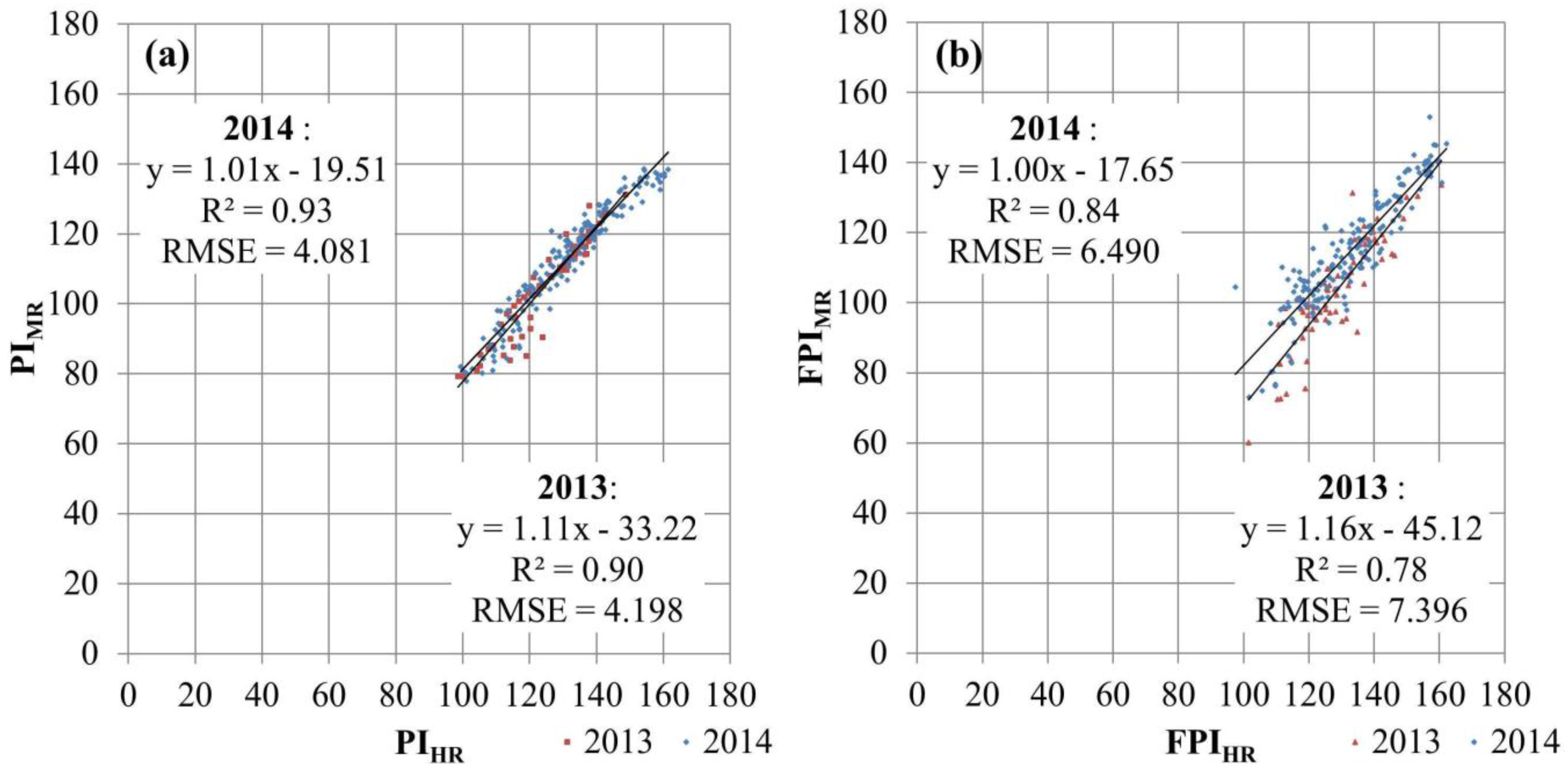
The agreement between FPI_MR and FPI_HR was examined. The indices were calculated for 2013 and 2014 over the same period (March 1 to October 23) according to the temporal coverage of the HR image time series used. The quality of the HR time series used to produce the reference data is discussed in relation with the results. The effect of the disaggregation step is addressed by comparing the characteristics of the linear regressions (slope, R², and RMSE) obtained between the HR and MR indices derived from whole pixel surfaces without land cover distinction (Production Index: PI_HR and PI_MR) or taking into account only grassland surface (FPI_HR and FPI_MR). This specific analysis is important in this study because it is assumed that disaggregation required by the use of MR images had a significant influence on the quality of biomass production estimation. To better understand the source of error, standardized residuals of the linear regressions between FPI_HR and FPI_MR are evaluated in relation to two characteristics of the ESU: the percentage of grassland within each ESU and the sampled grassland surfaces in the ESU to compute the FPI_HR.

Finally, the same analysis as the one conducted in the direct comparison was performed (cf. 2.2.4). In this case, the ΔFPI_MR was compared to the ΔFPI_HR (Equations (6) and (7)). The HR time series included images only from 2013 and 2014. Variation in biomass production in 2014 was quantified based on the one for 2013.

$$\Delta FPI{}_{MR}=\frac{FP{I}_{MR 2014}}{FP{I}_{MR 2013}}$$

(6)

$$\Delta FPI{}_{HR}=\frac{FP{I}_{HR 2014}}{FP{I}_{HR 2013}}$$

(7)

To better understand the level of error in estimates of ΔFPI_MR, the correlation between ΔFPI_MR and ΔFPI_HR was assessed while a threshold based on the grassland surface decreased the number of available ESU.

4.3. Results

4.3.1 Comparison of Annual Biomass Estimations Derived from HR and MR Product

Figure 9 illustrates the scatterplot MR indices and HR indices for 2013 and 2014.

The indicators (slope, R² and RMSE) used to characterize the linear regression all suggest a strong correlation between the MR and HR indices with R² values ranging from 0.78 to 0.93, slopes always equal or close to 1 (from 1.00 to 1.16), and RMSEs less than 8%. These results confirm those obtained with direct comparison that FPI derived from MR product could be considered as a suitable index to monitor annual biomass production variations. However, two main differences are observed.

The R² and the RMSE were consistently better in 2014 than in 2013 for both PI and FPI. This may be partly explained by differences in the number of ESUs processed (69 in 2013 and 173 in 2014) which depended on the quality (cloud cover) and the spatial coverage of HR images. Even with a potentially higher number of HR images in 2013 than in 2014 (26 vs. 22 images), the availability of HR images in 2013 was not consistent spatially and temporally. This is due to longer periods of cloud cover (greater than the 40 threshold used for interpolation of daily fCover between two dates) and a more variable spatial extent of HR images used. These results confirmed the importance of assessing the accuracy of the HR time series if it is used as reference data in MR product validation.

Figure 9. (a) Scatterplots of the Production Index (PI) and (b) Forage Production Index (FPI) derived from high resolution (HR) and moderate resolution (MR) images of 2013 and 2014. While PI indicates overall productivity without land cover distinction, FPI exclusively focuses on productivity in grassland.The HR and MR index values shown were obtained from 69 and 173 ESUs, respectively in 2013 and 2014. RMSE = Root Mean Square Error.

Figure 9. (a) Scatterplots of the Production Index (PI) and (b) Forage Production Index (FPI) derived from high resolution (HR) and moderate resolution (MR) images of 2013 and 2014. While PI indicates overall productivity without land cover distinction, FPI exclusively focuses on productivity in grassland.The HR and MR index values shown were obtained from 69 and 173 ESUs, respectively in 2013 and 2014. RMSE = Root Mean Square Error.

The R² and the RMSE were consistently better with indices calculated from fCover obtained without land cover distinction than when derived from an fCover based only on grassland pixels. This could be caused by the disaggregation process. Although disaggregation was required when monitoring grasslands with MR data, it could have a negative impact on the quality of the FPI_MR produced. Figure 10a illustrates the standardized residual of the linear regression between FPI_HR and FPI_MR in 2014 according to the percentage of grassland surface in all ESUs analyzed. The percentage of grassland had an influence on the performance of the disaggregation method with the variability of standardized residuals decreasing as the percentage of grassland increased (from 0.5% to 48%). This suggests that the performance of the FPI derived from the MR product will vary according to the proportion of grassland in a landscape. Further analysis is required to study the relation between the quality of FPI estimates and the grassland spatial heterogeneity (fragmented or continuous) [59,60]. To minimize the effect of the disaggregation step in the FPI_MR validation, it is recommended that ESU with a high percentage of grassland be sampled. This selection will necessarily induce a bias in the analysis and it will reduce the robustness of the validation regarding the ESU with little grassland. It is thus important to better define this threshold according to the level of error expected.

Regardless of the percentage of grassland within an ESU, part of the increase in the error measured on certainty in the FPI_MR based on fCover grassland pixels would have been associated with the quality of the reference data. The way to calculate the HR fCover for grasslands to produce the FPI_HR introduces a bias. If all grasslands in an ESU are used, or only a sample, consequences on the FPI_MR error are different. Figure 10b illustrates the standardized residual of the linear regression between FPI_HR and FPI_MR in 2014 according to the grassland sample rate in the ESU used to compute the FPI_HR. The bias introduced by the reference data is minimized if all grasslands within an ESU are accounted for because the heterogeneity of the grasslands within the ESU is better represented. In addition, this bias could be even more important depending on the quality of the data source used to identify the grasslands. For this latter point, investigation on the best data source is under way as no rule exists in the literature.

Figure 10. Standardized residuals of the linear regression for 2014 between FPI_MR and FPI_HR according to (a) the percentage of grassland surface in the ESU (for 173 ESUs of 3600 ha). (b) The percentage of grassland sampled to build the FPI_HR in the ESU (for 173 ESUs of 3600 ha).

Figure 10. Standardized residuals of the linear regression for 2014 between FPI_MR and FPI_HR according to (a) the percentage of grassland surface in the ESU (for 173 ESUs of 3600 ha). (b) The percentage of grassland sampled to build the FPI_HR in the ESU (for 173 ESUs of 3600 ha).

4.3.2. Comparison of Annual Biomass Ratio Derived from High Resolution and Moderate Resolution Products

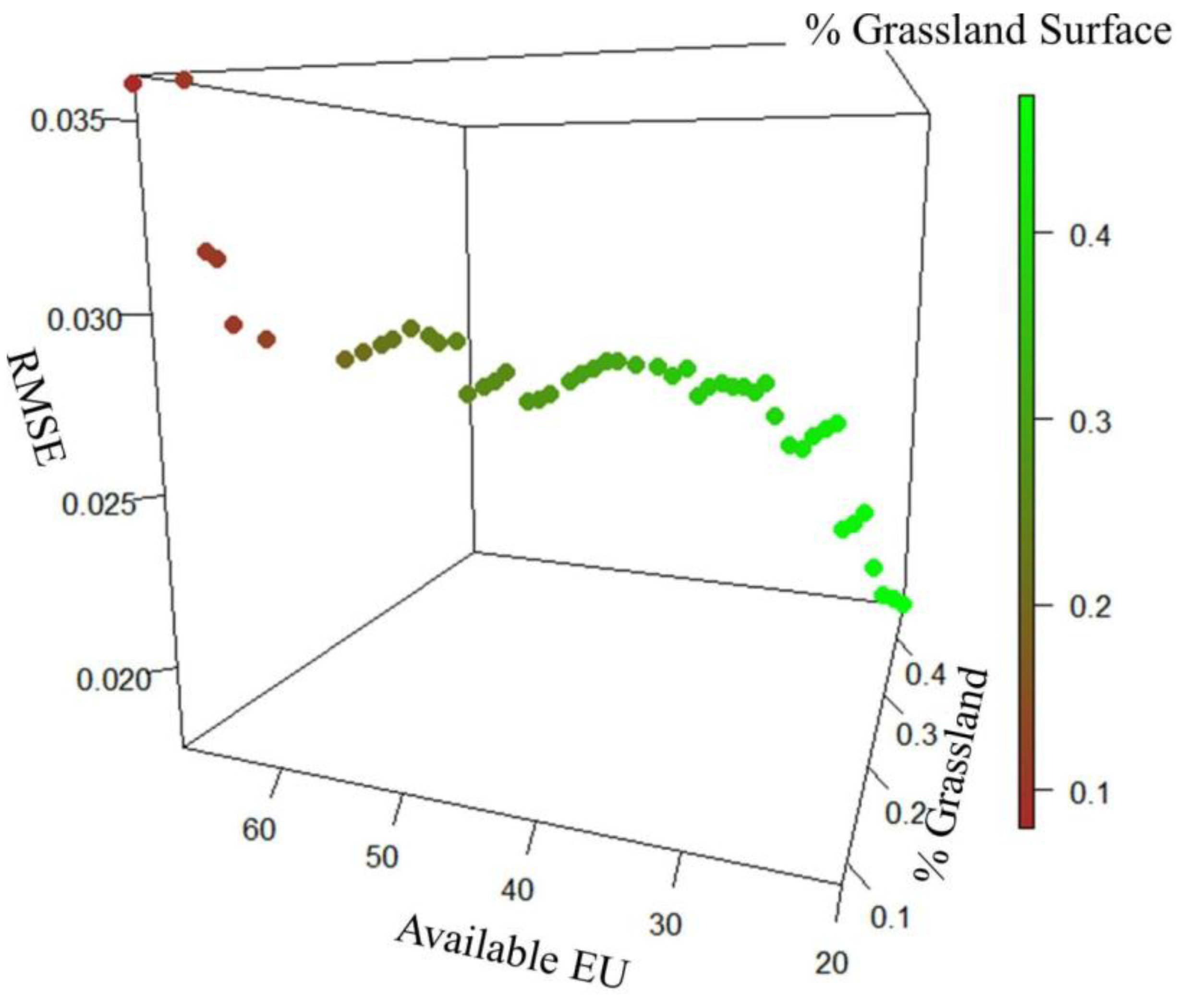
To analyze the effect of the grassland surface on the relationship between ΔFPI_MR and ΔFPI_HR, available ESUs were selected according to a threshold of the grassland surface. RMSE is subsequently calculated in each case. Figure 11 presents patterns of the RMSE according to the threshold of the grassland surface. RMSE decreases as the amount of grassland surface in the ESU increases. The number of available ESU decreases at the same time. It confirms the previous observations between annual biomass estimations (FPI_MR and FPI_HR) and highlights the importance of the grassland sampling strategy in the validation activity.

Even if the RMSE is acceptable (from 2% to 4%), the best coefficient of determination is low (R² = 0.33) compared to the one obtained from direct comparison (R² = 0.71). It was found with a sample of 28 ESUs and a minimum of 45% of grassland per ESU. A main reason is a small range of variability in biomass production observed between 2013 and 2014 (range of ΔFPI_MR = 0.15) compared to the one recorded between 2012 and 2013 (range of ΔFPI_MR = 0.59). Providing a conclusion based on this result is misleading. With the SPOT5 Take5 program conducted in 2015, the HR time series dataset could be enriched with an additional year (2013-2014-2015) providing a way to potentially get more interannual biomass production [61].

Figure 11. Root Mean Square Error of the linear regression for 2014 between ΔFPI_MR and ΔFPI_HR (Y-axis) according to the percentage of grassland surface in the ESU (Z-axis) and the available ESUs for the analysis according to the grassland surface threshold (X-axis).

Figure 11. Root Mean Square Error of the linear regression for 2014 between ΔFPI_MR and ΔFPI_HR (Y-axis) according to the percentage of grassland surface in the ESU (Z-axis) and the available ESUs for the analysis according to the grassland surface threshold (X-axis).

5. Discussion

A quality assessment of FPI derived from MODIS products and developed to support index-based forage production insurance in France was performed for three years (2012/2013/2014) over a limited geographic extent of two departments (Lot and Aveyron). Given the availability of MR vegetation index time series datasets within the scientific community, the number of index-based insurance products has increased. However, validation is often not performed. This work highlights why rigorous validation is critical before releasing a product to the user community.

Validating MR satellite products directly with biomass production data remains difficult. Given the various source of uncertainty in the data, results show satisfactory FPI accuracy (i.e., slope close to 1; R² between 0.78 and 0.93; RMSE less than 8%). Collecting sufficient production data with high quality biomass measurements to obtain a statistically meaningful dataset at the scale of a 6 km × 6 km ESU was very difficult. In this protocol, sampling rate was maximized by collecting biomass data from the highest number of plots possible (290 plots in 2012, 768 in 2013 and 557 in 2014). However, maximizing the sampling rate required use of biomass measurement methods that were less accurate than ones traditionally used at the plot level (e.g., mowers, mechanical and electronic plate meters). Despite these procedural decisions, the sampling rate within original ESUs remains low (below 2%). Resized ESUs were defined (from 3600 ha to 1152 ha) using the spatial distribution of grassland plots belonging to a set of farmers. At the scale of the ESU, this enabled reaching a reasonable sampling rate (an average of 13.2%). At the same time, however, it decreased the representativeness of the production data. Plots were not selected randomly in the ESU and often belonged to only one or two producers whose adopted management practices may have led to biomass production differences compared to other local operations.

The validation methodology applied here followed recommendations suggested in the context of the Committee on Earth Observing Satellites—Land Product Validation (CEOS LVP) sub-group for validation of remote sensing vegetation products. Upscaling the fCover value over a larger area was a meaningful way to decrease the influence of the signal coming from surrounding pixels while producing the HR fCover reference data [29,62]. Nevertheless, modifications to the validation guidelines were made based on the target variable (FPI_MR derived from MODIS fCover) and the scale of application (France). Results showed that FPI_MR could be used as a proxy to monitor annual biomass production of grasslands and its variations with a satisfactory levels of error. This suggests that FPI has reached validation stage level 1 according to CEOS-LVP criteria [28] and is now ready to be tested with the same methodology in other geographic contexts and compared with similar products (definition of validation stage level 2).

Considering the future availability of continuous HR time series data from platforms such as Landsat-8 and Sentinel-2, the accessibility of HR time series provided by the SPOT4 Take5 program was a good opportunity to test their potential for an index-based insurance product. Previous work with HR data yielded satisfactory results concerning the link between biomass and the integral of biophysical parameters like fAPAR or fCover [37,63]. With this study, the comparison of the FPI_MR with the FPI_HR provided additional important information about the strengths and weaknesses of such data. The two indices are highly correlated (R² = 0.78 and 0.84, respectively, for 2013 and 2014) and present a similar capacity to monitor interannual grassland biomass variation. However, using HR time series in the FPI processing chain avoids many issues caused by the use of MR images including disaggregation (direct observation of grassland surface), sampling (capacity to get fCover information on grasslands in ESUs with less than 15% grassland cover [64]), and validation (direct comparison with field measurements). On the other hand, other problems emerged. The consistency of FPI_HR relies on HR times series availability (space-time continuous data available at a national scale), the capacity to process images from different sensors to produce a robust biophysical variable [41], and the management of large datasets, all of which represent needs and active research questions.

In the case of the index-based insurance product, producing a ΔFPI with HR time series will not be possible before 2022, the time required to constitute a reference after the launch of both Sentinel-2 satellites in 2016. If needed, a possible transition could consist of using both HR and MR products by data fusion as it has been demonstrated that the precision of HR images and the repeatability of MR time series provide an optimal configuration for monitoring grassland production [65].

6. Conclusions

In the context of developing an index-based insurance product, this study presents a bottom-up approach for validating the use of an annual FPI as a surrogate for interannual biomass variation at a kilometric scale. Validating MR products remains challenging and constraining, especially given difficulties with ground data collection. Two protocols were designed to achieve a complete assessment of the FPI accuracy.

Direct comparison, where FPI_MR is compared with ground measurements of yield, led to good accuracy with R² = 0.71 and RMSE = 14.5%. The weakness of this analysis, the small number of ESU considered, is overcome by the indirect comparison approach. The HR time series, with images mainly from the SPOT4 Take 5 program and Landsat8 satellite, allow for an increase in the number of ESUs that can be processed (13 for the direct vs. 69 for indirect comparison). The relationships between HR and MR indices were quantified before disaggregation (PI_HR and PI_MR, R² = 0.90 and 0.93, respectively, for 2013 and 2014) and after (FPI_HR and FPI_MR, R² = 0.78 and 0.84, respectively, for 2013 and 2014). The percentage of grassland in the ESU was a key parameter for both variables. Whatever comparison is made, results showed that FPI can be improved by integrating meteorological variables to reduce remaining error [66]. The assimilation of farmer practices like the method and number of harvests or fertilization should also improve the accuracy of the FPI [67].

Moreover, given the pending release of Sentinel2 data, the feasibility of using HR sensors was discussed. This evolution in the processing chain is important and leads to mandatory modifications in data management. The interest in using HR time series is due primarily to elimination of the disaggregation step in the computation of FPI_MR [68]. Quantitative results and operational simulation of the final product are nevertheless still required. Moreover, prior to adopting data from new HR platforms, it is important to keep in mind that several years are needed to constitute a reference from Sentinel-2 data. Beyond index-based insurance, FPI may find other potential applications by providing information about local grassland production in near-real time for farmers to better manage their resources or for public authorities to assess regional production anomalies [69,70].