A Thin Plate Spline-Based Feature-Preserving Method for Reducing Elevation Points Derived from LiDAR

Abstract

Light detection and ranging (LiDAR) technique is currently one of the most important tools for collecting elevation points with a high density in the context of digital elevation model (DEM) construction. However, the high density data always leads to serious time and memory consumption problems in data processing. In this paper, we have developed a thin plate spline (TPS)-based feature-preserving (TPS-F) method for LiDAR-derived ground data reduction by selecting a certain amount of significant terrain points and by extracting geomorphological features from the raw dataset to maintain the accuracy of constructed DEMs as high as possible, while maximally keeping terrain features. We employed four study sites with different topographies (i.e., flat, undulating, hilly and mountainous terrains) to analyze the performance of TPS-F for LiDAR data reduction in the context of DEM construction. These results were compared with those of the TPS-based algorithm without features (TPS-W) and two classical data selection methods including maximum z-tolerance (Max-Z) and the random method. Results show that irrespective of terrain characteristic, the two versions of TPS-based approaches (i.e., TPS-F and TPS-W) are always more accurate than the classical methods in terms of error range and root means square error. Moreover, in terms of streamline matching rate (SMR), TPS-F has a better ability of preserving geomorphological features, especially for the mountainous terrain. For example, the average SMR of TPS-F is 89.2% in the mountainous area, while those of TPS-W, max-Z and the random method are 56.6%, 34.7% and 35.3%, respectively.

1. Introduction

The light detection and ranging (LiDAR) technique is currently one of the most prominent and effective tools for capturing high-density elevation data sets [1,2,3,4]. For example, the national wide raw LiDAR data in the Netherlands has approximately 640 billion points with the density of 6–10 points/m², and an approximately 1 km² of a Dublin city center point cloud has 225 million points with the density of 225 points/m² [5]. Such a huge amount of data always leads to serious time and memory problems in data processing, storage, visualization and transmission [6,7]. Thus, given the high density of LiDAR points, it is possible to substantially optimize data density and maintain the required accuracies of digital elevation models (DEMs). It should be noted that the points located on non-ground objects such as trees, buildings, cars and bridges in the raw LiDAR data set must be filtered before DEM generation [8]. Thus, our data density optimization method only deals with the randomly distributed ground points derived from LiDAR.

Data density optimization can generally be achieved by two schemes, i.e., progressive sampling and data reduction. The former attempts to maximize accuracy as efficiently as possible, starting with a small terrain points and using progressively larger ones until the terrain model reaches an acceptable accuracy level [9,10]. This method is relatively efficient when deriving points from photogrammetric mapping. Data reduction is achieved by selecting the most significant points from the raw data to best approximate the terrain surface in terms of some accuracy measures [11,12,13]. An excellent data reduction method should decrease the number of sample points without losing information about the described topography. Generally, data reduction ratio is much dependent on terrain characteristics. Namely, simple topographic roughness (e.g., flat terrain) needs a low data density to represent the morphology in comparison to complex morphologies with break slopes [14].

One of the key steps in the process of data reduction is to assess the importance of data points. A point is considered as ‘important’ when its elevation cannot be accurately interpolated using its neighbor sample points. Consequently, it will be included in the final terrain model. Various data reduction algorithms have been developed to generalize different forms of DEMs, such as contours, TIN and grid [11,15,16]. Lee [11] classified the existing algorithms into four groups: the skeleton, filter, hierarchy, and heuristic methods. Heckbert and Garland [17] categorized the algorithms into six groups, namely, regular grid, hierarchical subdivision, feature, refinement, decimation, and optimal methods. Cignoni et al. [18] classified the existing methods into seven groups: coplanar facets merging, mesh decimation, re-tiling, mesh optimization, vertex clustering, wavelet-based approaches and intermediate hierarchical representation. According to these fundamental principle and suitability for reducing 2.5D LiDAR-derived ground data, the existing algorithms can be classified as two groups: the point additional method and the point subtractive method.

The point additive method [12,19], also termed as maximum-z tolerance (max-Z), was originally derived from hierarchical triangulation, where a surface is approximated in a successively finer levels of detail by triangular patches whose projections in the horizontal plane are nested [20]. It guarantees that elevation differences between the original and the resulting TINs at any location are not more than a specified z tolerance. For dealing with LiDAR data set, max-Z first generates a candidate TIN using sufficient points to fully cover the perimeter of the original points. It then incrementally improves the TIN surface until it meets the specified z-tolerance. It does so by adding more points on an as-needed basis during an iterative process. Unfortunately, this method tends to produce long and thin TINs since it never alters previous results during the addition of points [11]. Furthermore, subtle terrain features located in flat areas are always omitted [21].

The point subtractive method is the reverse of the point additive one [11]. It starts a triangulation of all points and iteratively drops points from the triangulation until the threshold of simplification is reached [22,23,24]. During each iteration, all points are assessed, and the point which causes the least elevation difference when dropped will be eliminated. This method generally performs well. Yet, it is time consuming, especially for processing LiDAR data points with a high density. Similar to the point additive method, the subtractive method also misses the shape and topological relationships of drainage features, particularly in flat areas [21].

It can be concluded that almost all the classical data reduction methods use the simple linear interpolation methods to assess the importance of each candidate. This may lead to poor interpolation accuracy, especially for areas with complex topography. In order to overcome the shortcoming of linear interpolators, a greedy-based multiquadric (MQ) method (MQ-G) was recently developed for LiDAR-derived ground data reduction [25]. Numerical tests indicated that MQ-G is more efficient to select critical points than the classical methods including the random method and max-Z. Furthermore, MQ-G outperforms the other methods in retaining geomorphologic features based on the same number critical points (e.g., 100, 200, 400, 600, 800 and 1000). However, MQ-G is very time-consuming, as selecting one significant point requires the solution of an O (n³) system, where n is the number of pre-selected critical points. In addition, it does not do a good job for retaining geomorphological features, particularly in flat landscapes [25].

In digital terrain analysis, geomorphological feature lines are important terrain formations, since they accurately describe changes in surface smoothness or continuity [26,27]. Insertion of feature lines into the elevation grids is more prone to obtain morphologically and hydrologically enhanced DEMs, especially in flat landscapes [4,14,28,29,30]. In addition, when feature lines are included in DEMs, the number of points needed to represent the terrain can then be significantly reduced in the context of DEM generalization. Thus, many researchers [21,31,32] tried to insert feature lines into the generalized DEMs. However, this process is simply achieved with a constrained TIN.

In order to overcome the shortcoming of linear interpolation in critical point selection and feature line integration, the aim of this paper is to propose a TPS-based feature-preserving method (TPS-F). The TPS-F method iteratively evaluates the importance of all candidate points by computing these interpolation errors. The point with the largest interpolation error is regarded as the most significant and will be classified into the critical points. The process is repeated until the number of selected points reaches a pre-set level or no point is found to have the interpolation error exceeding a user-specified accuracy tolerance. In addition, by means of Australian National University DEM (ANUDEM) algorithm, geomorphological feature lines, extracted from the whole LiDAR ground points, are integrated into DEMs.

The advantages of taking TPS as the basis function are as follows:

• the interpolation accuracy of TPS is comparative to that of MQ, yet the former is much faster than the latter by means of some advanced algorithms to solve the finite difference form of TPS. For example, the discrete cosine transform (DCT)-based TPS has the computational complexity of O (n log (n)) [33].
• hydrological features can be easily incorporated into DEMs by the available variant of TPS, i.e., ANUDEM. This leads to the hydrologically corrected DEMs.

Thus, compared with MQ-G, our newly developed method (i.e., TPS-F) is not only fast, but also feature-preserving for LiDAR data reduction in the context of DEM construction. This greatly supports hydrological applications that depend on accurate representation of surface drainage structure, such as stream network modeling, catchment area computation and hydrological response prediction [34,35].

The remainder of this paper is organized as follows. The methodology of TPS-F is introduced in Section 2. In Section 3, four study sites with different morphologies are employed to compare the performance of TPS-F with those of the classical methods including TPS-based algorithm without feature lines (TPS-W), max-z tolerance (max-Z) and the random method. The only difference between TPS-F and TPS-W is whether the feature lines are integrated into DEMs. Discussion and conclusions are respectively given in Section 4 and Section 5.

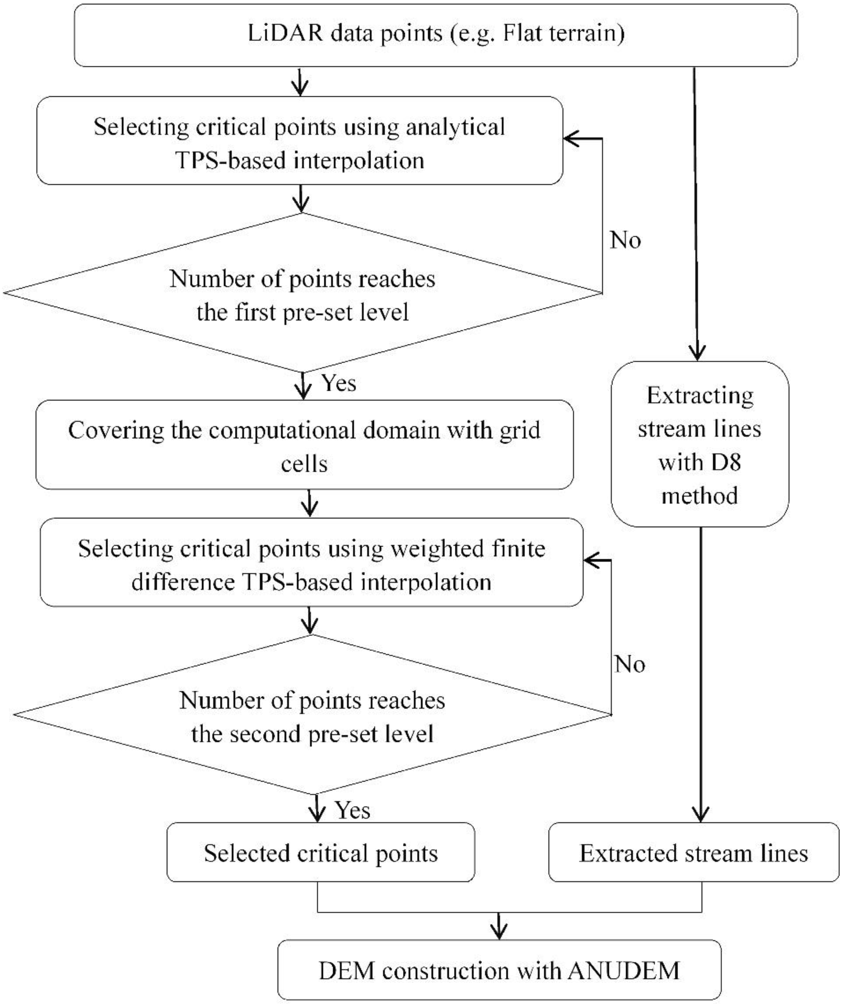
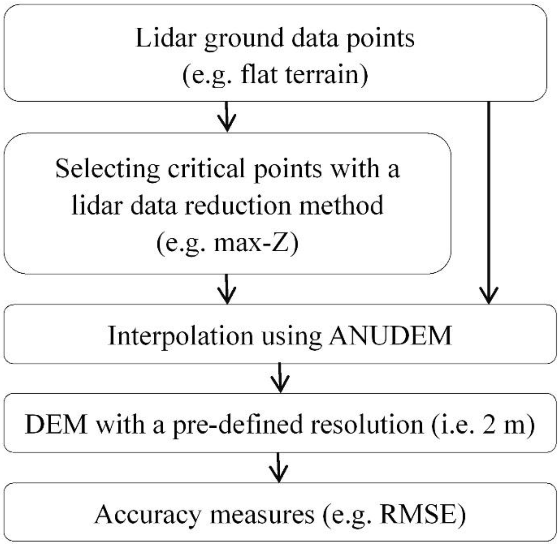
2. Proposed LiDAR Data Reduction Method

2.1. Thin Plate Spline (TPS)

In statistics and data analysis, smoothing is used to reduce experimental noise or small-scale information while keeping the most important features of a dataset [36]. Consider the following model for noisy sampling value f(x_i) at point x_i,

$$\left[f\left(x_i\right)=h\left(x_i\right)+e\left(x_i\right),i=1,2,\cdots ,n\right]$$

(1)

where e(x_i) is the random error term with zero mean and unknown variance, which is due to random measurement error and short range micro-scale variation that occurs over a range below the resolution of the dataset; h(x_i) is supposed to be the smoothed value of f(x_i); n is the number of sample points. Theoretically, TPS minimizes a criterion function that balances the tradeoff between the fidelity to the data and a smoothness penalty term that represents the roughness of the function estimate. This leads to the following regularized least-squares problem:

$$\left[\underset{h}{\min }{\displaystyle \sum _{i=1}^n{\left(f\left(x_i\right)-h\left(x_i\right)\right)}^2}+sP\left(h\right)\right]$$

(2)

where s is the smoothing parameter; P(h) represents the penalty term. For the two-dimensional Cartesian coordinate space (x, y), P(h) is expressed as,

$$\left[P\left(h\right)={\displaystyle {\int }_{R^2}\left(h_{xx}^2+2h_{xy}^2+h_{yy}^2\right)}dxdy\right]$$

(3)

where h_xx and h_yy are the second order partial derivatives of h(x, y) with respect to x and y, respectively, and h_xy is the cross partial derivative.

There are generally two approaches to fitting surfaces by means of TPS, namely analytical computation [37] and finite difference approximation [38]. For the former technique, the value of variable h at the ith position (x_i, y_i) can be expressed as a sum of two components [37]:

$$\left[h(x_i,y_i)={\displaystyle \sum _{j=1}^n{c}_{j}b(r_{ij})}+{\displaystyle \sum _{j=1}^k{d}_j{p}_j(x_i,y_i)}\right]$$

(4)

where r_ij is the distance from the interpolated point (x_i, y_i) to the jth sample point; b(r) is a radial basis function; p_j, j=1,…, k is a set of k polynomials forming the basis of polynomials; c_j and d_j are the coefficients, obtained by solving the following system of linear equations:

$$\left[\left(\begin{array}{cc}\mathit{B}+\raisebox{1ex}{$\mathit{I}$}\!\left/ \!\raisebox{-1ex}{$s$}\right.& \mathit{P}\\ {\mathit{P}}^T& 0\end{array}\right)\left(\begin{array}{c}\mathit{c}\\ \mathit{d}\end{array}\right)=\left(\begin{array}{c}\mathit{f}\\ 0\end{array}\right)\right]$$

(5)

where, $\mathit{B}=\left(\begin{array}{ccc}{b}_{11}& \cdots & b_{1n}\\ ⋮& \ddots & ⋮\\ b_{n1}& \dots & b_{nn}\end{array}\right)$; $b_{ij}=b\left(r_{ij}\right)$; $\mathit{c}=\left(\begin{array}{c}{c}_1\\ ⋮\\ c_n\end{array}\right)$; $\mathit{d}=\left(\begin{array}{c}{d}_1\\ ⋮\\ d_k\end{array}\right)$; $\mathit{f}=\left(\begin{array}{c}{f}_1\\ ⋮\\ f_n\end{array}\right)$.

In practice, the optimal value of the smoothing parameter s in Equation (5) is generally determined by the k-fold cross-validation algorithm [39].

For TPS, b(r) is expressed as,

$$\left[b(r)=r^2\log \left(r\right)\right]$$

(6)

Equation (5) indicates that the values of all candidate points can be directly estimated by the analytical TPS. Thus, the interpolation errors are the differences between the interpolated and sampled elevations. Considering the fact that the finite difference TPS is only valid in case of gridded data, the computational domain of the study site must be covered by grid cells with the resolution same to the DEM to be constructed when performing interpolations with finite difference TPS. Moreover, the values of the critical points, pre-selected by the analytical TPS, should be assigned to the corresponding grids where they are located. Thus, there are two groups of grids with and without values, which are termed known and unknown grids. The values of the unknown grids are estimated by the weighted finite difference TPS [33]. Therefore, the interpolation errors of candidate points are the elevation differences between the sampled points and the corresponding grids where they are located.

In case of gridded data, the principle of the weighted finite difference TPS is as follows. For the finite difference TPS in case of gridded data, the finite difference of P(h) can be expressed as,

$$\left[P\left(h\right)={\Vert \mathit{B}\mathit{h}\Vert }^2\right]$$

(7)

where h=[h₁₁ … h_1m h₂₁ … h_2m … h_n1 … h_nm]^T; n and m respectively represent the row and column of grid cells in the computational domain; B=(B₁, 2B₂, B₃)^T; B₁, B₂ and B₃ represent the second-order difference operators of h_xx, h_xy and h_yy, respectively; ||•|| is the norm computation.

For estimating the values of unknown grids, a weighted version of Equation (2) is used (i.e., weighted finite difference TPS) and its matrix formulation is expressed as,

$$\left[\underset{\mathit{h}}{\min }\left({\Vert {\mathit{W}}^{1/2}\left(\mathit{f}-\mathit{h}\right)\Vert }^2+s{\Vert \mathit{B}\mathit{h}\Vert }^2\right)\right]$$

(8)

where W is the diagonal matrix diag(w_i) that contains the weights w_i∈[0,1]. For the known grid, w=1, and for the unknown grid, w=0.

Minimizing Equation (8) with respect to h, we can obtain the following expression as,

$$\left[\mathit{W}\mathit{h}-\mathit{W}\mathit{f}+s{\mathit{B}}^T\mathit{B}\mathit{h}=0\right]$$

(9)

Or,

$$\left[\left(\mathit{W}+s{\mathit{B}}^T\mathit{B}\right)\mathit{h}=\mathit{W}\mathit{f}\right]$$

(10)

Equation (10) can be reformulated as,

$$\left[\left(\mathit{I}+s{\mathit{B}}^T\mathit{B}\right)\mathit{h}=\left(\mathit{I}-\mathit{W}\right)\mathit{h}+\mathit{W}\mathit{f}\right]$$

(11)

Equation (11) is always solved with an iterative procedure, which is expressed as,

$${\mathit{h}}^{i+1}={\mathit{H}}^{-1}\left(\mathit{W}\left(\mathit{f}-{\mathit{h}}^i\right)+{\mathit{h}}^i\right)$$

(12)

where i is the iterative times; H is the hat matrix, expressed as,

$$\left[\mathit{H}=\mathit{I}+s{\mathit{B}}^T\mathit{B}\right]$$

(13)

Direct solving Equation (12) has the computational complex of O ((n·m)³). Garcia [33] indicated that in case of gridded data, Equation (12) can be solved by means of the discrete cosine transform (DCT). Thus, Equation (12) can be reformulated as,

$$\left[{\mathit{h}}^{i+1}=\text{IDCT}\left(\mathit{\Omega }\text{DCT}\left(\mathit{W}\left(\mathit{f}-{\mathit{h}}^i\right)+{\mathit{h}}^i\right)\right)\right]$$

(14)

where DCT and IDCT refer to the discrete cosine transform and the inverse discrete cosine transform, respectively; Ω is a diagonal matrix with each nonzero element being the function of the smoothing parameter s and eigenvalues of B. The optimal value of s is determined by the generalized cross-validation (GCV), expressed as [33],

$$GCV(s)=\frac{{\Vert {\mathit{W}}^{1/2}\left(\mathit{h}-\mathit{f}\right)\Vert }^2/\left(m\cdot n-N_{\text{miss}}\right)}{{\left(1-\text{Tr}\left(\mathit{H}\right)/\left(m\cdot n\right)\right)}^2}$$

(15)

where N_miss is the number of unknown grid cells. Tr(H) is the trace of H. Theoretical and numerical tests showed that the computational cost of solving Equation (14) is O (n·m log(n·m)), which is much smaller than that of the direct method.

Theoretically, two sample points are enough to give a solution to (c, d) based on the analytical computation (i.e., Equation (5)). Thus, it is very suitable to perform interpolations at the beginning steps of critical point selection. However, with the increasing number of selected points, the computational cost of solving Equation (5) grows significantly. Moreover, for the irregularly distributed data points, Equation (5) is often numerically unstable due to the rank deficient of coefficient matrix. The above problems can be easily overcome by the finite difference approximation (i.e., Equation (14)) with gridded data. Hence, the two versions of TPS are respectively used for conducting interpolations in the process of critical point selection. Namely, we first perform interpolations using the analytical TPS, and then it will be replaced by the finite difference one when a certain number of critical points have been selected.

2.2. Selecting Critical Points Based on TPS-Based Algorithms

One of the main steps for selecting significant points is to assess the importance of all candidate points. In our study, we assume that a point is considered to be important if the elevation difference between the interpolated and sampled ones (i.e., interpolation error) exceeds a pre-defined tolerance. For example, according to the standard of digital products of fundamental geographic information 1:5000 DEM published by National Administration of Surveying, Mapping and Geoinformation of China in the year of 2010, the maximum error should not be bigger than 2 m and 10 m in the flat and hilly terrains, respectively. In our method, each point is interpolated with the pre-selected critical points. The point with the largest interpolation error is grouped into the critical points. The process is terminated when the number of selected points reaches a pre-defined level or when no point is found to have the interpolation error exceeding a user-specified tolerance.

The detailed steps for selecting critical points are as follows:

• Initial critical point selection. In principle, all LiDAR points can be considered as candidates for the critical points. The two data points with the maximum and the minimum elevations are first selected, as they are the most probable to be terrain feature points. Thus, there are two groups of dataset, i.e., critical points and candidate points.
• Performing interpolation to all candidate points by the analytical TPS with the pre-selected critical points. The interpolation errors of all candidate points are computed.
• Selecting the critical point. Based on above explanation, the point with the largest interpolation error is more important than others. Thus, it is selected as the critical point.
• Repeating 2 and 3 until the number of selected points reaches a pre-determined threshold (e.g., 100).
• Covering the computational domain of the study site using the grid cells whose resolution is same to the DEM to be constructed.
• Assigning the values of the pre-selected critical points to the grid cells where they are located.
• Performing interpolation by the weighted finite difference TPS. Thus, the values of the unknown grids are estimated.
• Computing interpolation error of each candidate point. We first find the grid cell where the candidate point locates, and then compute the elevation difference between the point elevation and the corresponding grid cell value. By means of this scheme, the location difference between the sample points and the corresponding central points of DEM grids can be avoided [40].
• Selecting the critical point whose interpolation error is the largest.
• Assigning the value of the newly selected critical point to the grid cell where it is located.
• Repeating (7) and (10) until the total number of selected points reaches a pre-specified level or the largest interpolation error is smaller than a pre-defined tolerance.

2.3. Hydrologically Corrected DEM Construction

In our method, ANUDEM, specifically designed for the creation of hydrologically corrected DEMs [28], was employed to merge the feature lines into DEMs. Key features of ANUDEM include its computational efficiency, allowing it to be applied to very large data sets, and a range of locally adaptive features, including a drainage enforcement algorithm that attempts to maintain connected drainage structure in the interpolated DEM, and algorithms to incorporate data streamlines, lakes and cliffs [41].

In our study, the stream lines are extracted from the LiDAR-derived DEM by using the simple D8 flow algorithm [42], and the feature-preserving DEMs are constructed using ANUDEM by taking the pre-selected critical points as the basis, supplemented with the incorporation of stream line data. In principle, the detail degree of stream network is controlled by the magnitude of the flow accumulation threshold. With a small threshold, a detailed stream network is formed, and vice versa. Based on ANUDEM, the extracted streamline can be accurately incorporated into DEMs [41]. Thus, flow accumulation threshold should be determined according to the required detail degree of stream network. In our following examples, the flow accumulation threshold is 1000.

The flow chart of TPS-F for LiDAR data reduction in the context of DEM construction is shown in Figure 1.

Figure 1. Flow chart of TPS-F for LiDAR data reduction in the context of DEM construction.

Figure 1. Flow chart of TPS-F for LiDAR data reduction in the context of DEM construction.

3. Materials and Results

3.1. Study Sites and LiDAR Data Collection

An area located in the Heihe River basin (HRB) in the arid region of northwest China was selected as the study site. HRB has approximately 1,432,000 km², located from 37.7°N to 42.7°N and from 97.1°E to 102.0°E. This basin is characterized by its distinct cold and arid landscapes: glaciers, frozen soil, alpine meadow, forest, irrigated crops, riparian ecosystem, and desert, which are distributed upstream to downstream [43]. In order to cover different topographies, four sites with different terrain morphologies (i.e., flat, undulating, hilly and mountainous terrains) were selected. The four sites are respectively characterized by flat terrain with some U-shaped gullies (Figure 2), by undulating land with prominent ridge and valley lines cross the area (Figure 3), by steep hilly slopes with a deep-cutting stream channel (Figure 4) and by mountainous terrain with an obvious ridge line (Figure 5). The four study sites have the same area of about 0.363 km² (i.e., 602 m × 602 m).

Figure 2. Distribution of the 100 critical points selected by (a) TPS-based algorithm, (b) max-Z and (c) the random method in the flat terrain.

Figure 2. Distribution of the 100 critical points selected by (a) TPS-based algorithm, (b) max-Z and (c) the random method in the flat terrain.

Figure 3. Distribution of the 100 critical points selected by (a) TPS-based algorithm, (b) max-Z and (c) the random method in the undulating terrain.

Figure 3. Distribution of the 100 critical points selected by (a) TPS-based algorithm, (b) max-Z and (c) the random method in the undulating terrain.

Figure 4. Distribution of the 100 critical points selected by (a) TPS-based algorithm, (b) max-Z and (c) the random method in the hilly terrain.

Figure 4. Distribution of the 100 critical points selected by (a) TPS-based algorithm, (b) max-Z and (c) the random method in the hilly terrain.

Figure 5. Distribution of the 100 critical points selected by (a) TPS-based algorithm, (b) max-Z and (c) the random method in the mountainous terrain.

Figure 5. Distribution of the 100 critical points selected by (a) TPS-based algorithm, (b) max-Z and (c) the random method in the mountainous terrain.

The raw data of all the study sites were sampled using Leica ALS70 with the laser wavelength of 1064 nm in the year of 2012. During data capture, for the flat site, the relative flying height was about 1500 m with the mean data density of 4 point/m², and for the other three sites, the absolute flying height was about 4800 m with the mean data density of 1 point/m². TerraSolid’s TerraScan software was employed to classify the ground points from the non-ground LiDAR points. Here, we assumed that there were no non-ground points mixed in the ground ones. The number of ground points, the corresponding point post-spacing and some terrain characteristics of the four sites are listed in Table 1.

Table 1. Topography characteristics of the four study sites.

Terrain Statistics	Flat	Undulating	Hilly	Mountainous
Minimum elevation (m)	1405.8	3129.4	1003.2	3891.6
Maximum elevation (m)	1411.9	3384.2	1321.5	4214.4
Mean elevation (m)	1409.1	3241.8	1154.0	4048.8
Standard deviation (m)	1.23	55.2	67.57	74.34
Mean slope (°)	2.993	30.31	38.87	54.04
Terrain roughness	1.002	1.205	1.309	2.9469
Number of ground points	647,516	235,765	100,204	250,736
Point post-spacing (m)	1.3	1.6	1.9	1.2

Table 1. Topography characteristics of the four study sites.

Terrain Statistics	Flat	Undulating	Hilly	Mountainous
Minimum elevation (m)	1405.8	3129.4	1003.2	3891.6
Maximum elevation (m)	1411.9	3384.2	1321.5	4214.4
Mean elevation (m)	1409.1	3241.8	1154.0	4048.8
Standard deviation (m)	1.23	55.2	67.57	74.34
Mean slope (°)	2.993	30.31	38.87	54.04
Terrain roughness	1.002	1.205	1.309	2.9469
Number of ground points	647,516	235,765	100,204	250,736
Point post-spacing (m)	1.3	1.6	1.9	1.2

3.2. Accuracy Measures

In addition to TPS-based algorithms (i.e., TPS-F and TPS-W), the maximum z-tolerance (Max-Z) and the random method were also adopted for LiDAR data reduction. Theoretically, both TPS-based methods and Max-Z have two stopping rules, namely, the maximum interpolation error and the number of points to be selected. In our study, the latter stopping rule was employed to give a comparative analysis between all the data reduction methods since the random method cannot control its performance in terms of the maximum interpolation error. Based on the latter stopping rule, we want to show which method has the best accuracy for DEM construction with the same number of critical points. This can indirectly validate the efficiency of a method for capturing critical points. We respectively set the number of selected critical points as 0.1%, 0.2%, 0.4%, 0.6%, 0.8% and 1% of total number of LiDAR ground points.

Root mean square error (RMSE) and error range (i.e., maximum error minus minimum error) were used for accuracy comparison. The formulation of RMSE is as follows,

$$\left[\text{RMSE}=\sqrt{{\displaystyle \sum _{i=1}^N{\left(H_i-E_i\right)}^2}/N}\right]$$

(16)

where H and E respectively represent the DEMs constructed by all LiDAR points (original DEM) and by the selected critical points (reduced DEM); N is the total number of DEM grids. In our study, the DEM resolution is 2 m, which is approximate to the post-space of LiDAR data points.

Additionally, we also employed mean slope ($\overline{S}$) and terrain roughness (K) to assess the effect of all data reduction methods on preserving the morphological nature of the terrain surface. They are respectively expressed as [21],

$$\left[\overline{S}={\displaystyle \sum _{i=1}^N{S}_i\times A_i}/{\displaystyle \sum _{i=1}^N{A}_i}\right]$$

(17)

$$\left[K={A/A}_p={\displaystyle \sum _{i=1}^N{A}_i\sec S_i}/{\displaystyle \sum _{i=1}^N{A}_i}\right]$$

(18)

where S is the slope, measured in degrees; A_p is the projected area; A is the surface area, i is the ith grid cell; and N is the total number of the grid cells. In principle, the larger the mean slope and surface roughness, the better the data reduction method for preserving morphological nature on the reduced DEMs. Thus, good reduction methods should keep the two measures as large as possible.

In order to quantitatively measure the effectiveness of the aforementioned methods for retaining terrain features, streamline matching rate (SMR) was also adopted [21]. Its expression is as follows,

$$\left[\text{SMR}=L_r\times 100/L\right]$$

(19)

where L_r is the length of feature lines located in the corresponding feature line buffers; L is the total length of the original feature lines. Practically, the original feature lines such as ridges and valleys were first retrieved from the original DEM to generate ‘buffers’ with a threshold. Then the buffer zones were overlaid with the feature lines retrieved from the reduced DEMs. A large SMR means a high accuracy for feature-preserving. In this paper, the buffer threshold was 4 m, and hydrology module in ArcGIS 10.1 was used to extract feature lines.

Figure 6 shows the flow chart of the scheme used to assess the accuracy of data reduction methods.

Figure 6. Flow chart of the scheme used to assess the accuracy of data reduction methods.

Figure 6. Flow chart of the scheme used to assess the accuracy of data reduction methods.

3.3. Results

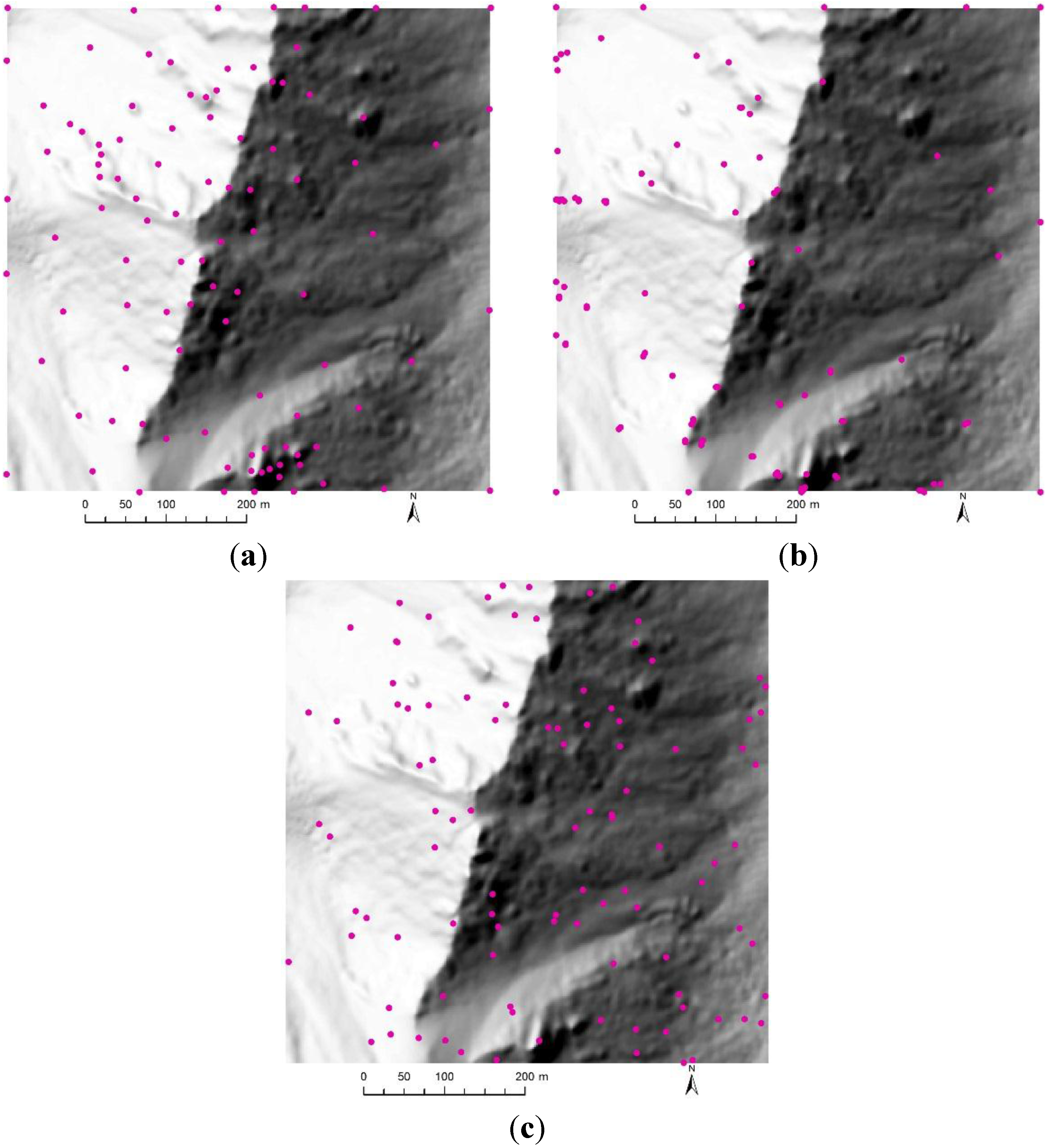
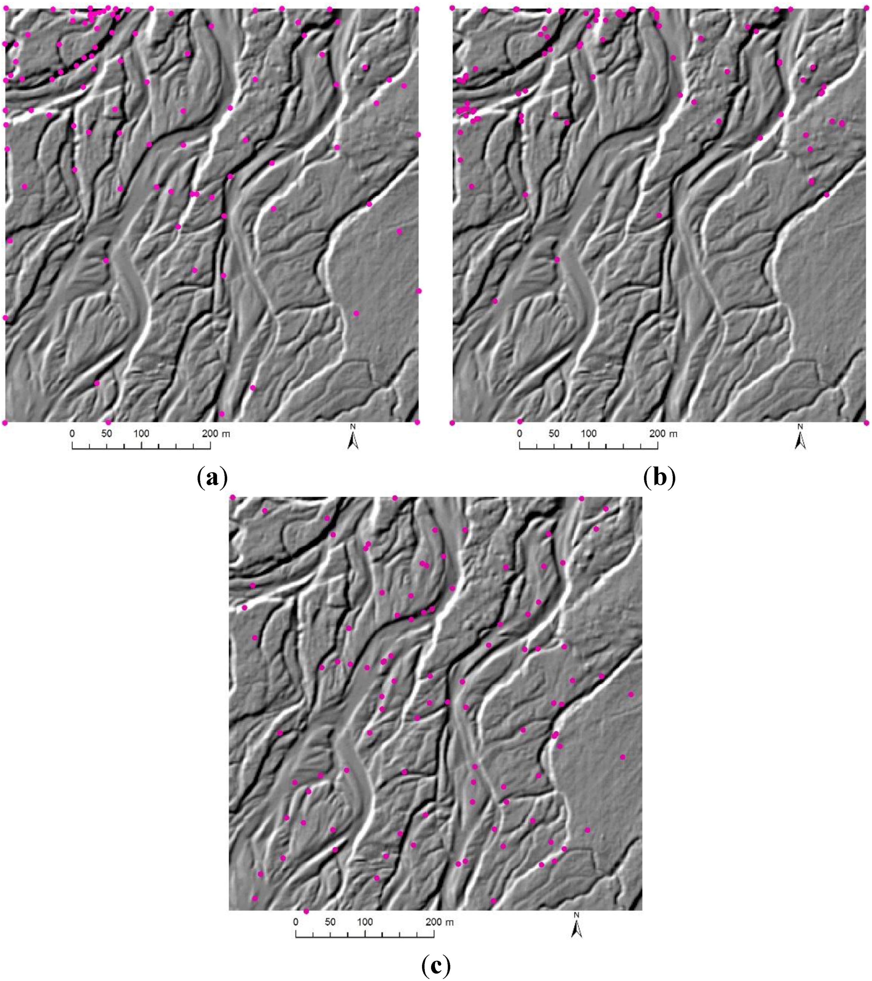
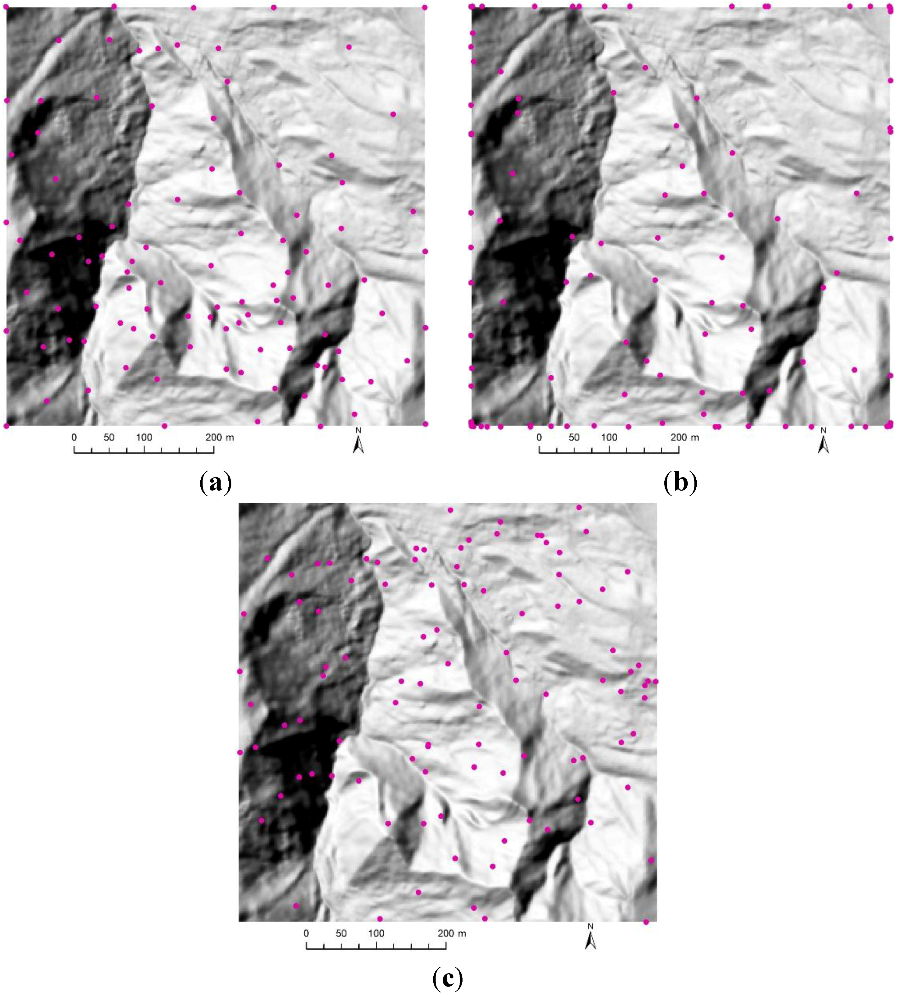
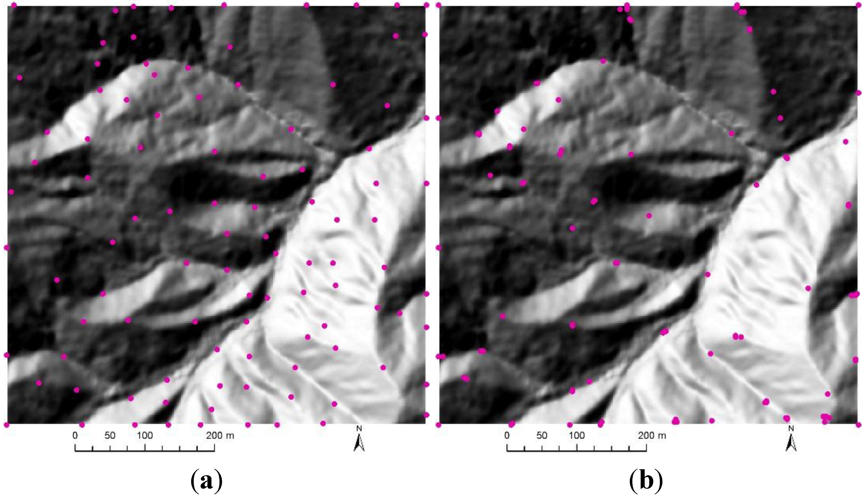
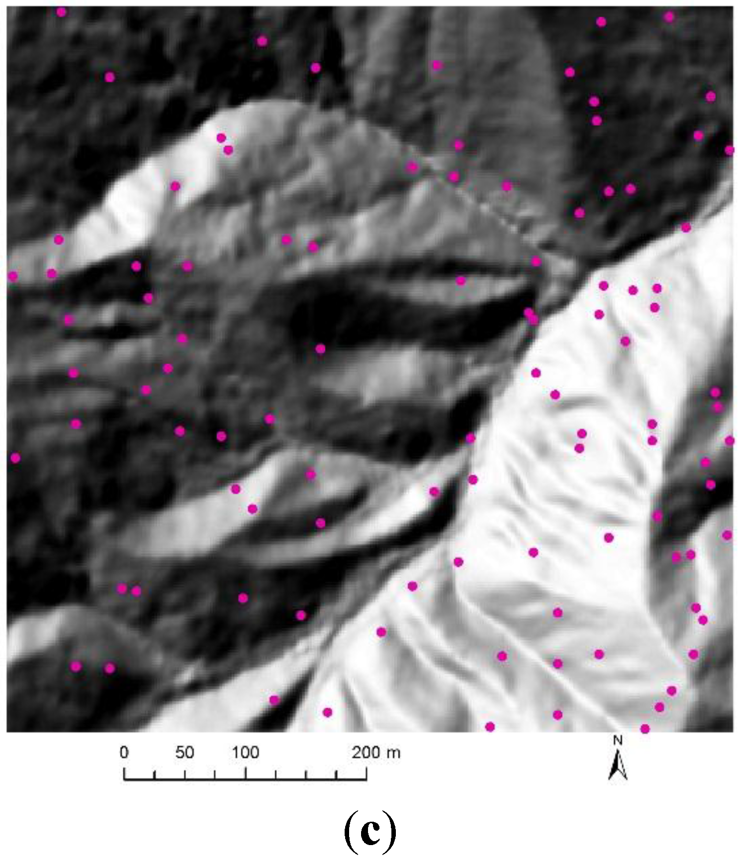
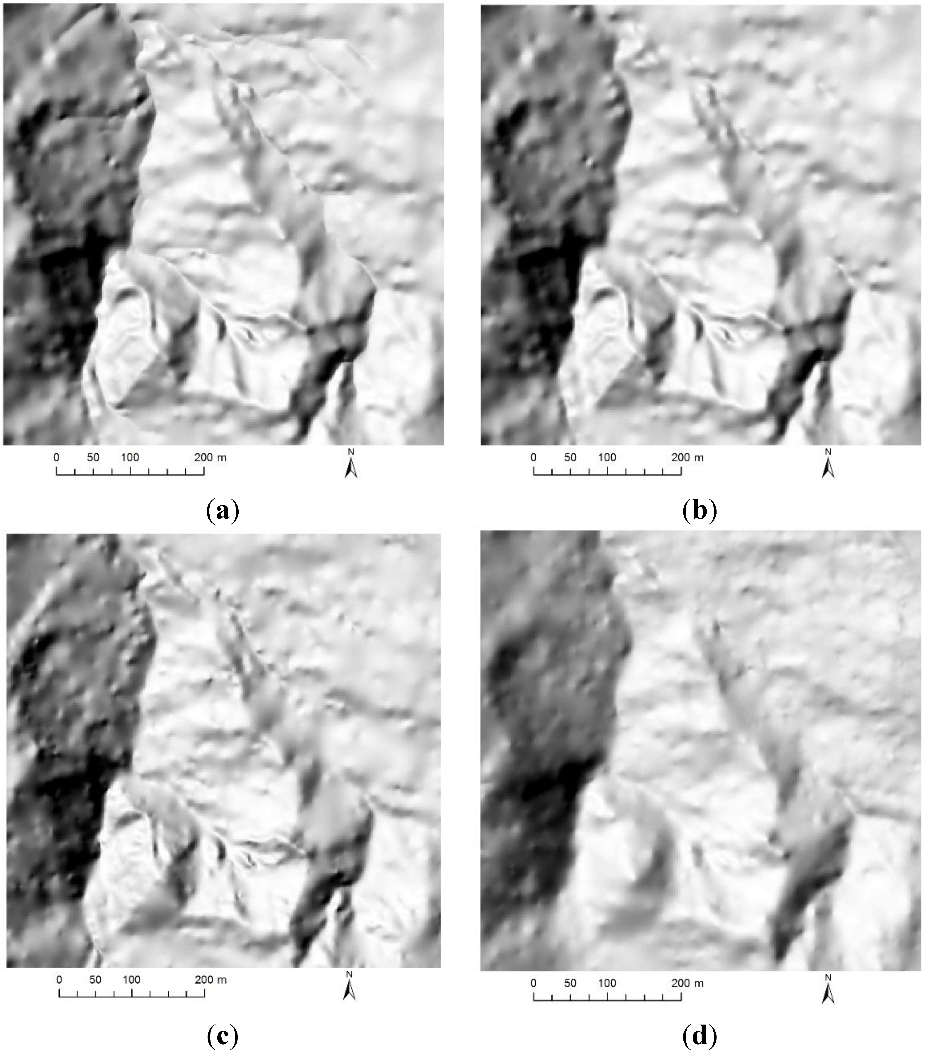
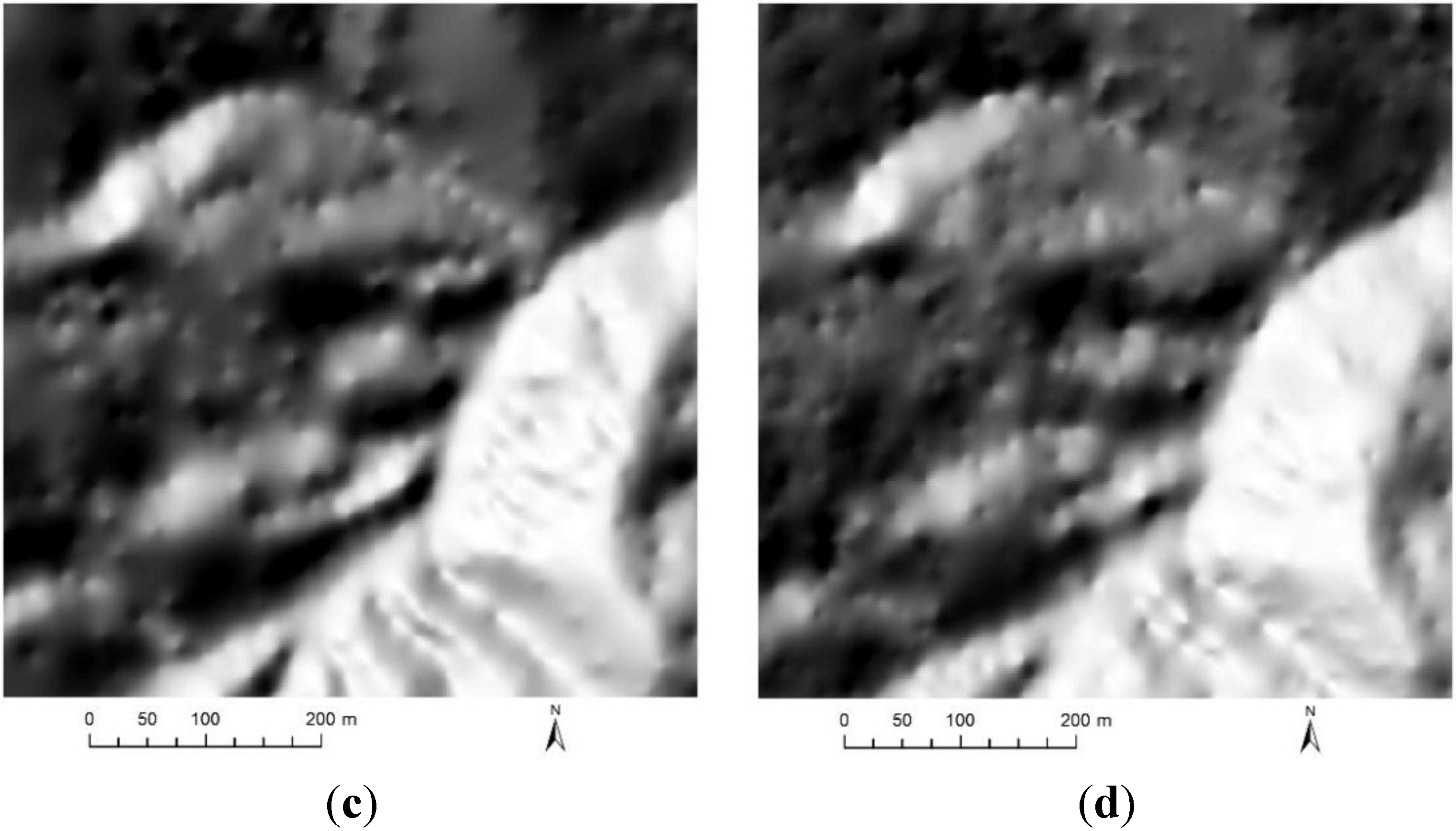
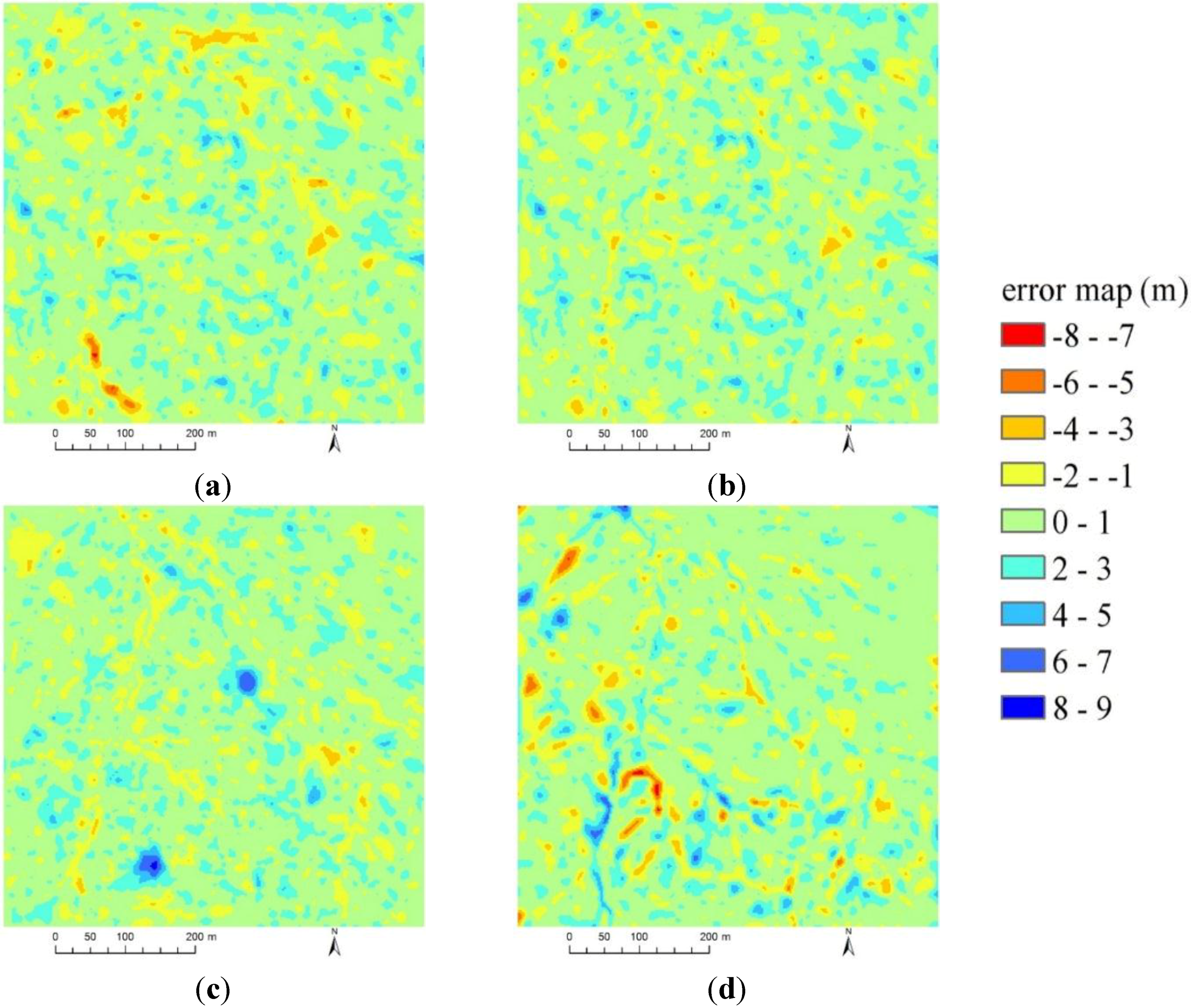
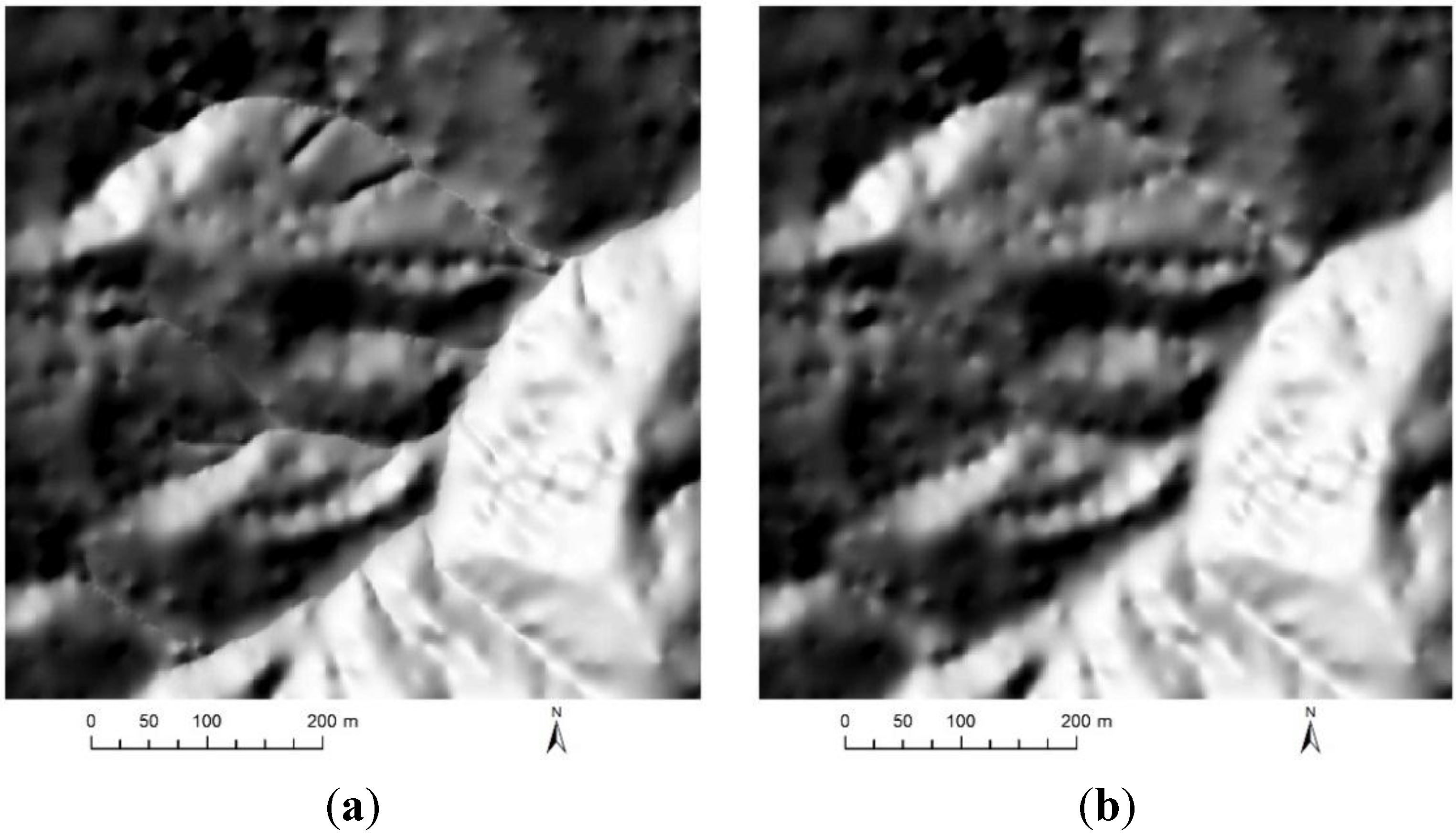
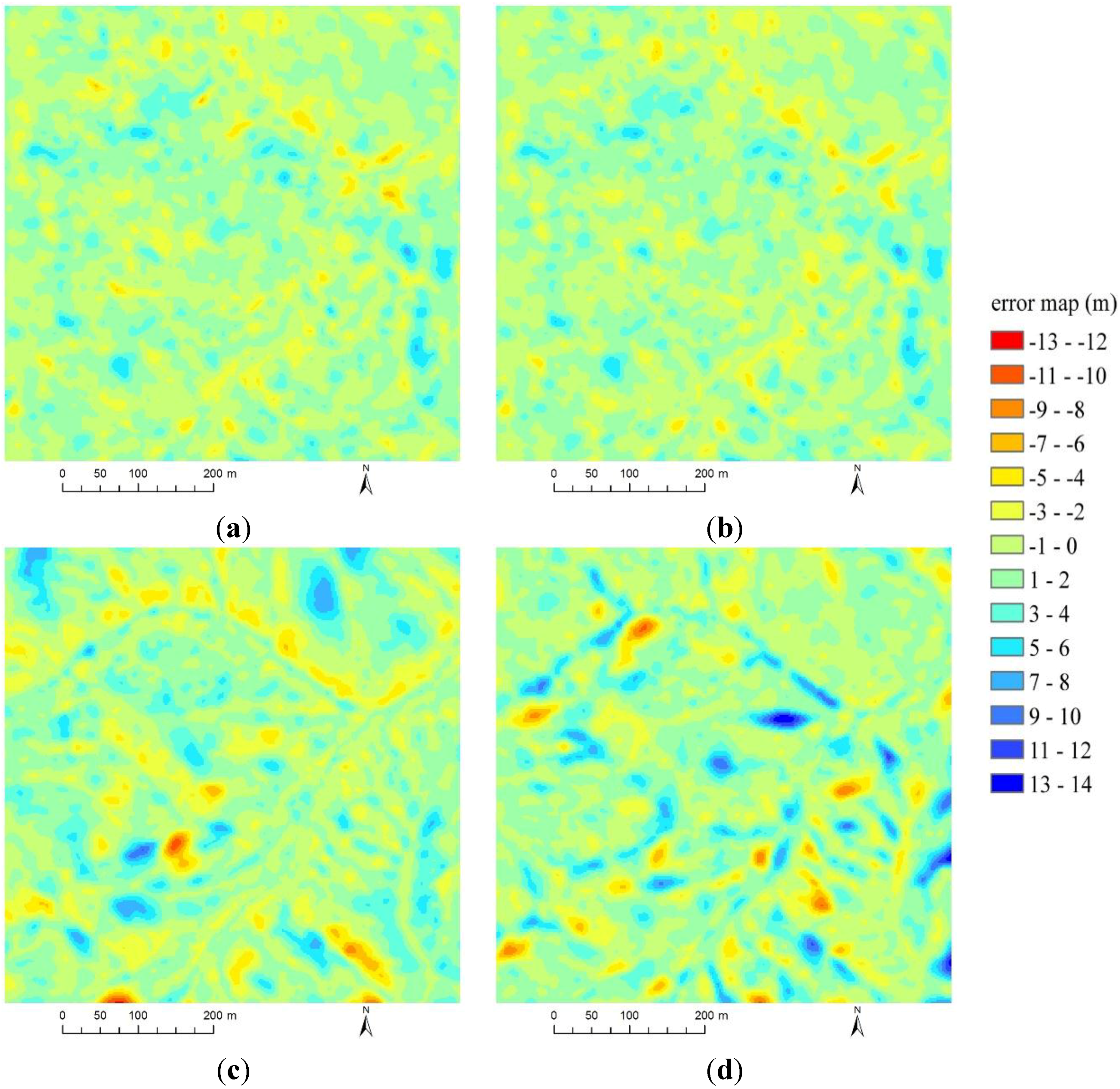
3.3.1. Qualitative Analysis

Figure 2, Figure 3, Figure 4 and Figure 5 show the distribution of 100 critical points selected by the random method, max-Z and TPS-based algorithm in the four study sites. It can be found that TPS-based algorithm tends to select more points located in complex areas than in flat areas. For example, the geomorphological features including the valleys (Figure 2a, Figure 3a and Figure 4a) and ridges (Figure 3a, Figure 4a and Figure 5a) are accurately captured by the TPS-based method. The points selected by max-Z tend to locate in the boundaries of the study sites, especially in the undulating area (Figure 3b). This is due to the poor interpolation accuracy of TIN at the sides of triangle than within the triangle [44]. Furthermore, many points are close to each other with an overly uneven distribution (Figure 2b and Figure 5b), which may make some points redundant for DEM construction. Due to the inherent nature, the points selected by the random method are evenly distributed across the whole study area without considering any geomorphological features Figure 2c, Figure 3c, Figure 4c and Figure 5c). Yet, this may lead to its high interpolation accuracy.

Specifically, for the flat site (Figure 2), the left-upper area is relatively complex. Thus, more points are captured by both TPS-based method (Figure 2a) and max-Z (Figure 2b) in this area. Compared with max-Z, TPS-based algorithm has four additional points located in the flat terrain (i.e., right-middle area). This can guarantee the high interpolation accuracy for DEM construction. For the undulating site (Figure 3), both TPS-based algorithm and max-Z have many points to describe the prominent ridge and valley lines. However, the former (Figure 3a) has more points located in the subtle terrain (e.g., left-bottom area) than the latter (Figure 3b). Similar conclusions are also obtained from the hilly site (Figure 4). For example, TPS-based algorithm is more accurate than max-Z for describing the subtle terrain in the left and bottom areas. Relatively, the mountainous area (Figure 5) has a much coarser appearance than the others, as there are many isolated peaks. It can be found that almost all these peaks are captured by TPS-based algorithm, yet most of them are omitted by max-Z. In summary, the points captured by TPS-based method are more effective than those by max-Z for describing terrain features.

The hillshades of TPS-F, TPS-W, max-Z and the random method with 1% of LiDAR points in the undulating and hilly sites are respectively shown in Figure 7 and Figure 8. It can be found that regardless of data reduction methods, the reduced surfaces are much coarser than the original ones. This is due to the low data density used for DEM construction. However, the prominent terrain features are well kept. Irrespective of terrain complexity, the random method always obtains the poorest results with the heavily blurred terrain features (Figure 7d and Figure 8d). For example, in the undulating site, the valley in the right and the subtle ridges in the bottom are lost (Figure 7d). In the hilly site, the subtle ridges in the right completely disappear (Figure 8d). Max-Z is more accurate than the random method. Yet, it has an obvious pit-filling problem in the two sites (Figure 7c and Figure 8c). Furthermore, for the undulating site, the left area is much coarse with many isolated peaks (Figure 7c). Comparatively, TPS-based methods seem more accurate than the others for keeping morphological features. Moreover, TPS-F has better results than TPS-W. For example, in the undulating site, the valleys in the right and upper are accurately captured by TPS-F, and all valley bottoms of TPS-F are much narrower than those of TPS-W.

Error maps (i.e., elevation difference between the reduced and original DEMs) in the undulating and hilly sites are provided in Figure 9 and Figure 10. It can be found that irrespective of terrain morphology and data reduction method, DEM error is always spatially variable. The random method has more extreme errors than the other methods (Figure 9d and Figure 10d). This indicates that the random method does not accurately capture the morphological features. Max-Z performs slightly better than the random method. However, the former also omits some peaks and pits, proved by many large errors (Figure 9c and Figure 10c). The two versions of TPS obtain similar error maps. Yet, some large negative errors can be found in the map of TPS-F in the undulating site (Figure 9a). This may be due to the fact that ANUDEM gives a biased change to elevations in different spatial patterns and magnitudes to better reflect known hydrology [29].

Figure 7. Hillshades of (a) TPS-F, (b) TPS-W, (c) max-Z and (d) random with1% of LiDAR points in the undulating site.

Figure 7. Hillshades of (a) TPS-F, (b) TPS-W, (c) max-Z and (d) random with1% of LiDAR points in the undulating site.

Figure 8. Hillshades of (a) TPS-F, (b) TPS-W, (c) max-Z and (d) random with1% of LiDAR points in the hilly site.

Figure 8. Hillshades of (a) TPS-F, (b) TPS-W, (c) max-Z and (d) random with1% of LiDAR points in the hilly site.

Figure 9. Error maps of (a) TPS-F, (b) TPS-W, (c) max-Z and (d) random with1% of LiDAR points in the undulating site.

Figure 9. Error maps of (a) TPS-F, (b) TPS-W, (c) max-Z and (d) random with1% of LiDAR points in the undulating site.

Figure 10. Error maps of (a) TPS-F, (b) TPS-W, (c) max-Z and (d) random with1% of LiDAR points in the hilly site.

Figure 10. Error maps of (a) TPS-F, (b) TPS-W, (c) max-Z and (d) random with1% of LiDAR points in the hilly site.

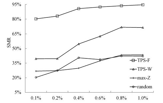
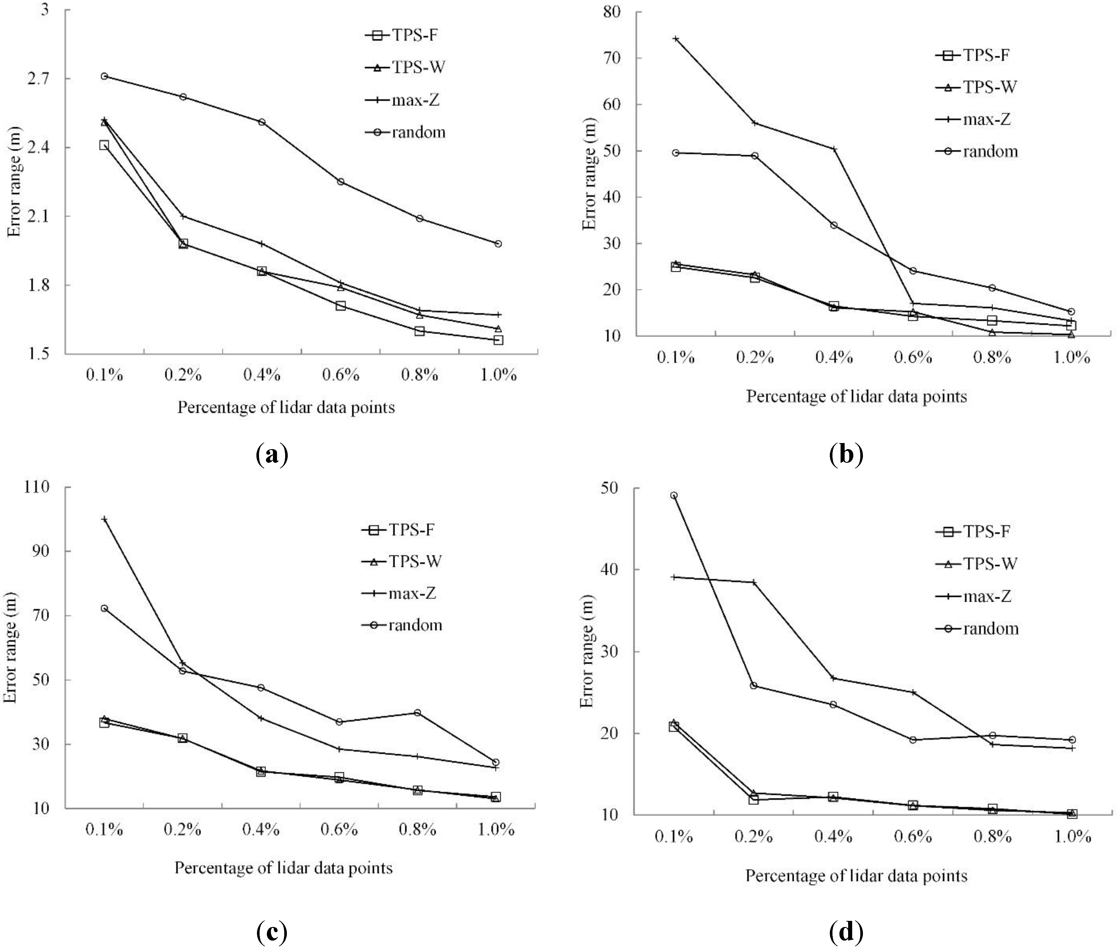
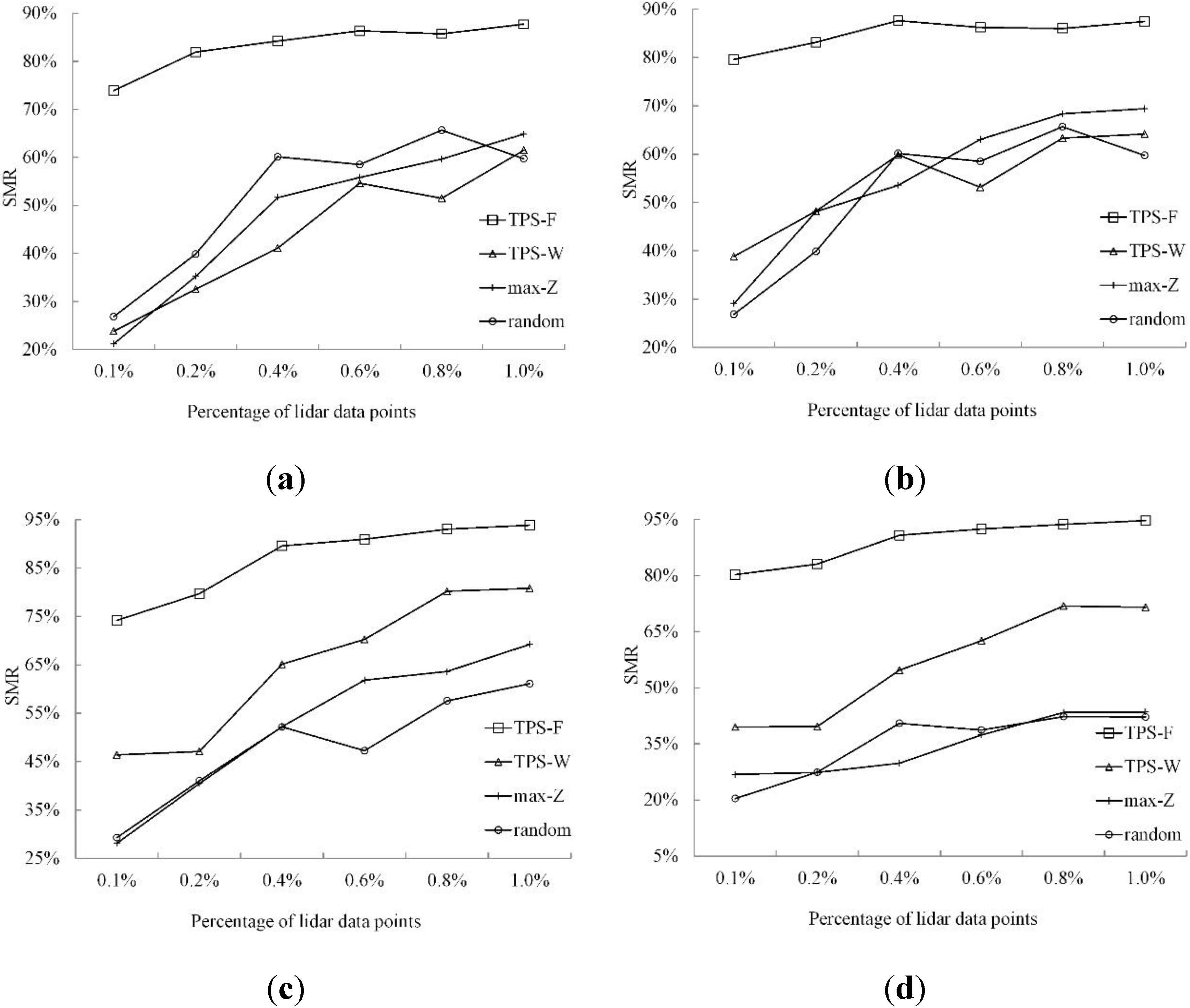
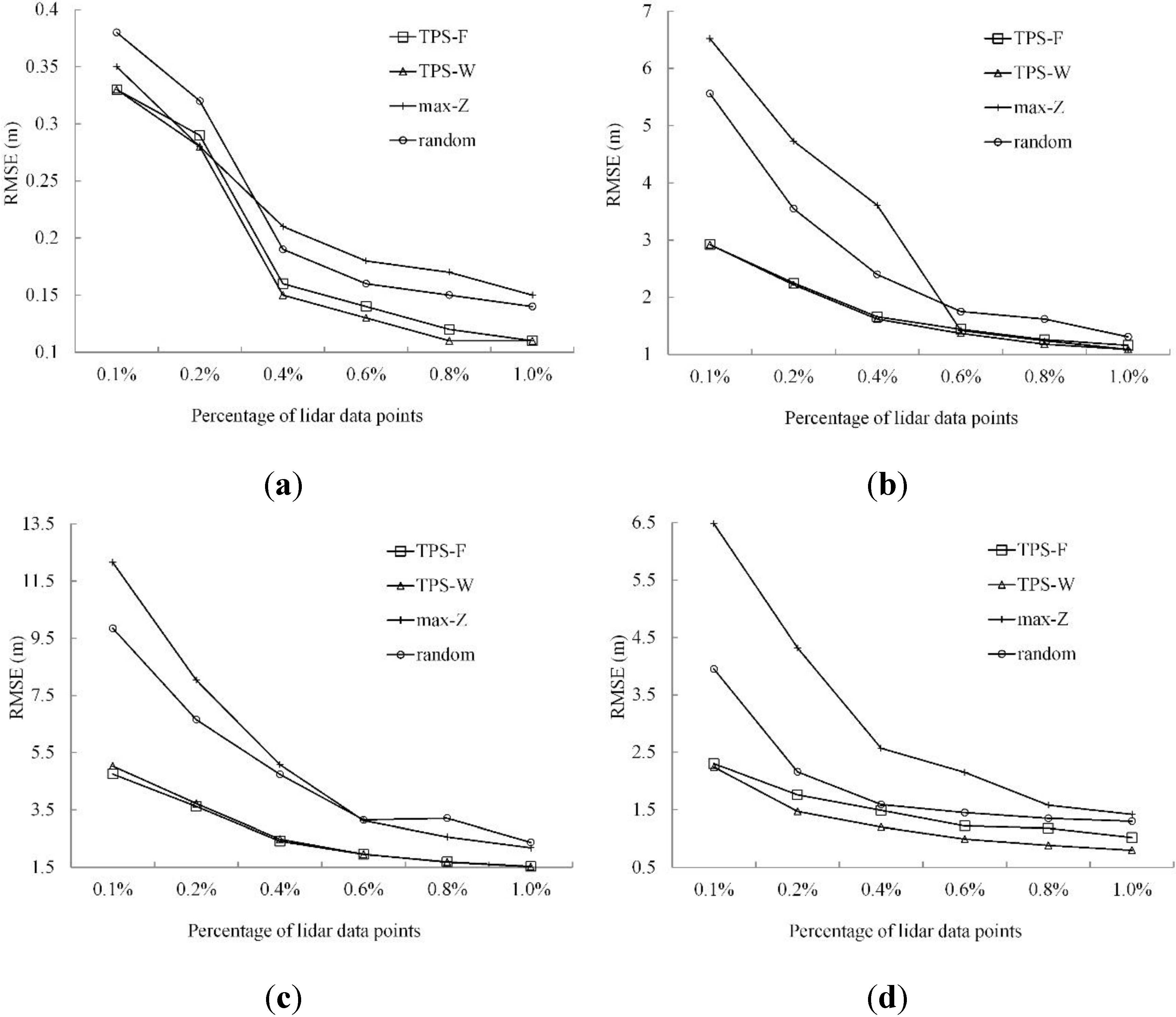
3.3.2. Quantitative Analysis

Here, accuracy measures including error range (maximum error minus minimum error), RMSE, mean slope and terrain roughness were respectively employed to compare the performances of all aforementioned data reduction methods. Moreover, SMR was also adopted to quantitatively assess how well the stream lines retrieved from the reduced DEMs match those from the original DEM.

Figure 11 shows the relationship between error range and number of selected critical points under different terrain morphologies. It can be found that with the increasing number of selected critical points, the error ranges of almost all methods decrease, except for the random method in hilly and mountainous areas. This indicates the unstable performance of the random method. The random method performs better than max-Z in the undulating and mountainous sites for a certain amount of critical points. This may be due to the uneven distribution of data points selected by max-Z (Figure 2b, Figure 3b, Figure 4b and Figure 5b). The two versions of TPS (i.e., TPS-F and TPS-W) are always more accurate than the random method and max-Z, especially for the hilly and mountainous terrains. For example, in the flat terrain, the error range of TPS-F ranges from 1.56 m to 2.41 m, while those of max-Z and the random method range from 1.67 m to 2.52 m and from 1.98 m to 2.71 m, respectively. Thus, we can conclude that the TPS-based algorithms can accurately capture terrain feature points.

Figure 11. Comparison of percentage of LiDAR data points (i.e., ratio of the number of selected critical points to the whole number of LiDAR points) versus error range between the four methods in the sites with (a) flat, (b) undulating, (c) hilly and (d) mountainous terrains.

Figure 11. Comparison of percentage of LiDAR data points (i.e., ratio of the number of selected critical points to the whole number of LiDAR points) versus error range between the four methods in the sites with (a) flat, (b) undulating, (c) hilly and (d) mountainous terrains.

Comparison of percentage of LiDAR data points versus RMSE between the four methods in all the study sites are provided in Figure 12. The RMSEs of almost all methods become smaller when the number of critical points increases. This result can be expected as the larger number of data points always leads to the more correct surface description [45]. Compared with max-Z, the random method performs well due to its even distribution of data points (Figure 2c, Figure 3c, Figure 4c and Figure 5c). The two versions of TPS are more accurate than the other methods at almost all study sites, especially for the hilly terrain. It should be noted that irrespective of terrain morphology, TPS-W always performs better than TPS-F. This is due to the fact that ANUDEM achieves the hydrologically corrected DEMs at the cost of biasedly changing a certain number of elevations [29].

Figure 12. Comparison of percentage of LiDAR data points (i.e., ratio of the number of selected critical points to the whole number of LiDAR points) versus RMSE between the four methods in the sites with (a) flat, (b) undulating, (c) hilly and (d) mountainous terrains.

Figure 12. Comparison of percentage of LiDAR data points (i.e., ratio of the number of selected critical points to the whole number of LiDAR points) versus RMSE between the four methods in the sites with (a) flat, (b) undulating, (c) hilly and (d) mountainous terrains.

Mean slope and terrain roughness of the four methods in all the study sites are given in Table 2 and Table 3. Irrespective of terrain morphology and data selection method, the mean slope becomes bigger with the increasing number of data points (Table 2). The average mean slopes of TPS-F are bigger than those of the other methods in almost all terrains, except for the flat terrain. For example, in the mountainous terrain, the average mean slope of TPS-F is 34.80°, while those of TPS-W, max-Z and the random method are 34.41°, 34.29° and 33.81°, respectively. Similar conclusions are also obtained in terms of terrain roughness (Table 3). In conclusion, TPS-F is more accurate than the other methods for preserving the geomorphological nature of the terrain surface.

The SMRs of all the methods in the four study sites are given in Figure 13. Irrespective of terrain morphology, TPS-F always performs better than the other methods in terms of SMR. On average, TPS-F obtains the lowest SMR in the flat terrain with the value of 83.3%, while the values of TPS-W, max-Z and the random method are 44.2%, 48.1% and 51.8%, respectively. The largest SMR of TPS-F is 89.2% in the mountainous area, while those of TPS-W, max-Z and the random method are 56.6%, 34.7% and 35.3%, respectively. All those results further prove the good performance of TPS-F for retaining terrain features.

Table 2. Mean slope of TPS-F, TPS-W, max-Z and the random method in the four study sites with different percentages of LiDAR data points (unit: degree (°)).

Terrain Morphology	Percentage of LiDAR Data Points	Method
		TPS-F	TPS-W	Max-Z	Random
Flat	0.1%	2.21	2.13	1.88	1.08
	0.2%	2.45	2.42	2.11	1.27
	0.4%	2.66	2.71	2.43	1.44
	0.6%	2.76	2.84	2.54	1.53
	0.8%	2.84	2.85	2.61	1.62
	1.0%	2.86	2.89	2.62	1.64
	On average	2.63	2.64	2.36	1.43
sUndulating	0.1%	29.74	29.18	26.70	26.38
	0.2%	29.93	29.37	27.63	27.25
	0.4%	30.14	29.74	28.39	28.04
	0.6%	30.36	30.05	29.97	28.36
	0.8%	30.42	30.27	30.06	28.53
	1.0%	30.51	30.39	30.16	28.72
	On average	30.18	29.84	28.82	27.88
Hilly	0.1%	36.52	35.54	33.09	31.33
	0.2%	37.93	37.19	35.45	33.02
	0.4%	38.31	37.66	36.64	34.64
	0.6%	38.61	38.17	37.11	35.59
	0.8%	38.75	38.37	37.41	35.86
	1.0%	38.78	38.44	37.77	36.50
	On average	38.15	37.56	36.24	34.49
Mountainous	0.1%	34.03	33.13	33.89	33.27
	0.2%	34.44	34.40	34.07	33.35
	0.4%	34.91	34.61	34.35	33.99
	0.6%	35.02	34.74	34.43	33.94
	0.8%	35.07	34.78	34.49	34.09
	1.0%	35.32	34.81	34.53	34.20
	On average	34.80	34.41	34.29	33.81

Table 2. Mean slope of TPS-F, TPS-W, max-Z and the random method in the four study sites with different percentages of LiDAR data points (unit: degree (°)).

Terrain Morphology	Percentage of LiDAR Data Points	Method
		TPS-F	TPS-W	Max-Z	Random
Flat	0.1%	2.21	2.13	1.88	1.08
	0.2%	2.45	2.42	2.11	1.27
	0.4%	2.66	2.71	2.43	1.44
	0.6%	2.76	2.84	2.54	1.53
	0.8%	2.84	2.85	2.61	1.62
	1.0%	2.86	2.89	2.62	1.64
	On average	2.63	2.64	2.36	1.43
sUndulating	0.1%	29.74	29.18	26.70	26.38
	0.2%	29.93	29.37	27.63	27.25
	0.4%	30.14	29.74	28.39	28.04
	0.6%	30.36	30.05	29.97	28.36
	0.8%	30.42	30.27	30.06	28.53
	1.0%	30.51	30.39	30.16	28.72
	On average	30.18	29.84	28.82	27.88
Hilly	0.1%	36.52	35.54	33.09	31.33
	0.2%	37.93	37.19	35.45	33.02
	0.4%	38.31	37.66	36.64	34.64
	0.6%	38.61	38.17	37.11	35.59
	0.8%	38.75	38.37	37.41	35.86
	1.0%	38.78	38.44	37.77	36.50
	On average	38.15	37.56	36.24	34.49
Mountainous	0.1%	34.03	33.13	33.89	33.27
	0.2%	34.44	34.40	34.07	33.35
	0.4%	34.91	34.61	34.35	33.99
	0.6%	35.02	34.74	34.43	33.94
	0.8%	35.07	34.78	34.49	34.09
	1.0%	35.32	34.81	34.53	34.20
	On average	34.80	34.41	34.29	33.81

Interpolation plays an important role in the quality of a DEM, especially with sparse LiDAR samples [6,46,47]. Thus, four classical interpolation methods including triangular with linear interpolation (TIN), inverse distance weighting (IDW), kriging with pre-fitted variogram and minimum curvature (MC) were also employed to construct DEMs with 1% percent of LiDAR points in the four study sites, and these results were compared with those of ANUDEM. Table 4 shows that regardless of terrain morphology, ANUDEM is always more accurate than the classical interpolation methods. ANUMDE has the best and the worst accuracy in the flat and hilly sites with the RMSEs of 0.11 m and 1.52 m, respectively. Averagely, ANUDEM is about 1.05, 3.25, 1.80 and 6.07 times as accurate as TIN, IDW, kriging and MC, respectively. The above results further prove the efficiency of ANUDEM used for LiDAR data reduction.

Table 3. Terrain roughness of TPS-F, TPS-W, max-Z and the random method in the four study sites with different percentages of LiDAR data points.

Terrain Morphology	Percentage of LiDAR Data Points	Method
		TPS-F	TPS-W	Max-Z	Random
Flat	0.1%	1.0012	1.0011	1.0009	1.0003
	0.2%	1.0015	1.0014	1.0011	1.0003
	0.4%	1.0018	1.0018	1.0015	1.0005
	0.6%	1.0019	1.0020	1.0016	1.0005
	0.8%	1.0020	1.0020	1.0017	1.0006
	1.0%	1.0020	1.0020	1.0017	1.0006
	On average	1.0017	1.0017	1.0014	1.0005
Undulating	0.1%	1.1950	1.1889	1.1434	1.1416
	0.2%	1.2002	1.1949	1.1584	1.1528
	0.4%	1.2042	1.2013	1.1688	1.1640
	0.6%	1.2067	1.2042	1.2030	1.1710
	0.8%	1.2073	1.2061	1.2049	1.1726
	1.0%	1.2079	1.2076	1.2057	1.1767
	On average	1.2036	1.2005	1.1807	1.1631
Hilly	0.1%	1.2722	1.2588	1.2227	1.1931
	0.2%	1.2973	1.2857	1.2587	1.2172
	0.4%	1.3029	1.2932	1.2734	1.2381
	0.6%	1.3086	1.3022	1.2810	1.2540
	0.8%	1.3106	1.3051	1.2848	1.2567
	1.0%	1.3108	1.3061	1.2910	1.2662
	On average	1.3004	1.2919	1.2686	1.2376
Mountainous	0.1%	1.2282	1.2128	1.2262	1.2106
	0.2%	1.2338	1.2332	1.2295	1.2133
	0.4%	1.2452	1.2388	1.2304	1.2220
	0.6%	1.2481	1.2410	1.2307	1.2213
	0.8%	1.2495	1.2416	1.2309	1.2238
	1.0%	1.2552	1.2417	1.2311	1.2255
	On average	1.2433	1.2349	1.2298	1.2194

Table 3. Terrain roughness of TPS-F, TPS-W, max-Z and the random method in the four study sites with different percentages of LiDAR data points.

Terrain Morphology	Percentage of LiDAR Data Points	Method
		TPS-F	TPS-W	Max-Z	Random
Flat	0.1%	1.0012	1.0011	1.0009	1.0003
	0.2%	1.0015	1.0014	1.0011	1.0003
	0.4%	1.0018	1.0018	1.0015	1.0005
	0.6%	1.0019	1.0020	1.0016	1.0005
	0.8%	1.0020	1.0020	1.0017	1.0006
	1.0%	1.0020	1.0020	1.0017	1.0006
	On average	1.0017	1.0017	1.0014	1.0005
Undulating	0.1%	1.1950	1.1889	1.1434	1.1416
	0.2%	1.2002	1.1949	1.1584	1.1528
	0.4%	1.2042	1.2013	1.1688	1.1640
	0.6%	1.2067	1.2042	1.2030	1.1710
	0.8%	1.2073	1.2061	1.2049	1.1726
	1.0%	1.2079	1.2076	1.2057	1.1767
	On average	1.2036	1.2005	1.1807	1.1631
Hilly	0.1%	1.2722	1.2588	1.2227	1.1931
	0.2%	1.2973	1.2857	1.2587	1.2172
	0.4%	1.3029	1.2932	1.2734	1.2381
	0.6%	1.3086	1.3022	1.2810	1.2540
	0.8%	1.3106	1.3051	1.2848	1.2567
	1.0%	1.3108	1.3061	1.2910	1.2662
	On average	1.3004	1.2919	1.2686	1.2376
Mountainous	0.1%	1.2282	1.2128	1.2262	1.2106
	0.2%	1.2338	1.2332	1.2295	1.2133
	0.4%	1.2452	1.2388	1.2304	1.2220
	0.6%	1.2481	1.2410	1.2307	1.2213
	0.8%	1.2495	1.2416	1.2309	1.2238
	1.0%	1.2552	1.2417	1.2311	1.2255
	On average	1.2433	1.2349	1.2298	1.2194

Table 4. RMSEs of triangular with linear interpolation (TIN), inverse distance weighting (IDW), kriging with pre-fitted variogram and minimum curvature (MC) in the four study sites (unit: m).

Terrain Morphology	ANUDEM	TIN	IDW	Kriging	MC
Flat	0.11	0.14	0.15	0.24	0.23
Undulating	1.09	1.13	3.16	1.26	4.11
Hilly	1.52	1.55	5.62	3.62	6.67
Mountainous	0.80	0.87	2.52	1.22	10.36
On average	0.88	0.92	2.86	1.59	5.34

Table 4. RMSEs of triangular with linear interpolation (TIN), inverse distance weighting (IDW), kriging with pre-fitted variogram and minimum curvature (MC) in the four study sites (unit: m).

Terrain Morphology	ANUDEM	TIN	IDW	Kriging	MC
Flat	0.11	0.14	0.15	0.24	0.23
Undulating	1.09	1.13	3.16	1.26	4.11
Hilly	1.52	1.55	5.62	3.62	6.67
Mountainous	0.80	0.87	2.52	1.22	10.36
On average	0.88	0.92	2.86	1.59	5.34

Figure 13. SMRs of TPS-F, TPS-W, max-Z and the random methods in the study sites with (a) flat, (b) undulating, (c) hilly and (d) mountainous terrains.

Figure 13. SMRs of TPS-F, TPS-W, max-Z and the random methods in the study sites with (a) flat, (b) undulating, (c) hilly and (d) mountainous terrains.

4. Discussion

Recently, Chen et al. [25] proposed a greedy-based MQ method (MQ-G) for LiDAR data reduction. Numerical tests indicated that regardless of terrain characteristics and number of selected critical points, MQ-G is more accurate than max-Z and the random method for DEM construction. However, MQ-G does not perform well for keeping terrain features, especially in flat terrain. For example, Chen et al. [25] showed that in the flat terrain with 1000 critical points, the SMR of MQ-G is only about 34.5%. However, our present study shows that irrespective of the number of critical points, the SMR of TPS-F is consistently bigger than 70%. Moreover, since DCT was employed to solve the finite difference form of TPS, TPS-based methods is much faster than MQ-G. Taking 400 points selection as an example, the computational cost of TPS-based algorithms is about 7.277 s, while that of MQ-G is about 144.45 s. Namely, our new method is about 19.85 times as fast as MQ-G. In summary, compared with MQ-G, TPS-F is not only faster at selecting critical points, but also has higher accuracy for keeping terrain features.

Similar to MQ-G, TPS-F is also impossible to determine the optimal number of data points under a required DEM accuracy. In practice, this problem can be solved by two approaches. The first one is the trial-and-error scheme. Namely, we repeatedly change the number of data points until the DEM accuracy reaches the pre-defined level. This method is time consuming yet simple. A more efficient approach is to establish relationships between DEM accuracy and accuracy influencing factors based on some empirical and theoretical models. For example, Aguilar et al. [46] gave empirical investigations on the effect of topographical variability and sample density on the accuracy of DEMs with respect to different interpolation methods. Kraus et al. [48] presented an empirical model based on moving least squares to deduce the local and relative accuracy measures for every interpolated grid point in DTMs, such as point density, terrain curvature and the number and alignment of the neighboring original points. Hence, based on the aforementioned models, the optimal number of points for constructing DEMs under a required accuracy can be determined.

In principle, our method can be grouped into the interpolated-based approach. At present, this kind of approach has been widely used for LiDAR filtering, such as the linear prediction-based method proposed by Kraus and Pfeifer [49], TIN-based filtering method developed by Axelsson [50], the despike virtual deforestation (VDF) algorithm presented by Haugerud and Harding [51], the regularized spline with tension (RST)-based method developed by Evans and Hudak [52], and the parameter-free (PF) method presented by Mongus and Žalik [53]. All the above methods adopted a similar scheme to achieve filtering. Namely, the DEM is first generated with an interpolation method (such as TPS, TIN, RST) and then the elevation difference between the previous and the current DEMs are computed and used for LiDAR filtering. Yet, there are some differences between the methods from a technical perspective. The differences between the PF method and our newly developed method are as follows:

• Purpose and available LiDAR data. The purpose of PF is to filter the raw LiDAR data including ground and non-ground points and to obtain a DEM. Our purpose is to reduce the huge amount of LiDAR-derived ground points to solve the serious time and memory consumption problems in the context of DEM construction.
• Ground seed selection. The PF method selects ground seeds by a local minimum method. Thus, there are many initial seeds including ground and non-ground points. Yet, there are only two ground seeds in our method. Namely, the points with the maximum and minimum elevations.
• DEM resolution. The PF method uses three levels of DEMs with the resolutions from fine to coarse. Yet, in the first step, our method performs interpolations to each candidate with the pre-selected ground points without using grid cells. In the second step, our method only use one level of grid cells with the resolution same to the resultant DEM.
• TPS computation. The PF method only uses a local analytical TPS to perform interpolations. Yet, our method respectively employs the analytical and finite difference TPSs to perform interpolations in the process of critical point selection and uses the ANUDEM to incorporate feature lines into DEMs. Moreover, all the three versions of TPS are used in a global form.

In addition to the above three versions of TPS, finite element TPS was also considered as a promising interpolator to perform interpolations. For example, Roberts et al. [54] presented a finite element TPS-based smoother, which combines the favorable properties of finite element surface fitting with the ones of thin plate splines. This method can deal with very large data sets consisting of tens of millions of predictor and response observations. Thus, in TPS-F, this method may replace the finite difference TPS for performing interpolations in LiDAR data reduction.

Theoretically, the quality of the DEM is largely a function of the accuracy, density and distribution of data points, terrain morphology, and interpolation method. Thus, there have been many studies on the accuracy of interpolation techniques for the generation of DEMs in relation to landform types. However, difference conclusions have been obtained. For example, Aguilar et al. [46] showed that Multiquadric Radial Basis Function (RBF) is considered as the best interpolation method, regardless of terrain morphology. Chaplot et al. [55] found that when the sample density is high, few differences exist between the interpolation methods. However, kriging obtains the best results for landscapes with strong spatial structure, low coefficients of variation (CV) and low anisotropy, while regularized spline with tension has the best estimations for landscapes with low CV and weak spatial structure. Under the conditions of high CV, strong spatial structure and strong anisotropy, IDW performs slightly better than the other methods. In fluvial geomorphology, many authors [14,56,57,58] found that TIN is more reliable to DEM construction. Guo et al. [59] indicated that regardless of terrain variability, simple interpolation methods, such as IDW, natural neighbor (NN), and TIN, are more efficient at generating DEMs from LiDAR data, but kriging-based methods are more reliable if accuracy is the most important consideration. Chu et al. [47] found that the performances of landslide scarp detection on the basis of various DEMs for kriging and TIN are better than those of IDW, particularly in sparse sample sizes. In our paper, we indicated that in terms of RMSE, ANUDEM is more accurate than the other methods, regardless of terrain morphology.

In our tests, we respectively set the number of selected critical points as 0.1%, 0.2%, 0.4%, 0.6%, 0.8% and 1% of total number of LiDAR ground points. The purpose of this scheme is not to replace the whole LiDAR points with only the selected ones, but to compare the efficiency of all data reduction methods for selecting critical points in the context of DEM construction.

5. Conclusions

In this paper, we have developed a TPS-based feature-preserving method (TPS-F) for LiDAR-derived ground data reduction in the context of DEM construction. Firstly, two versions of TPS solution methods including analytical and finite difference ones were respectively employed to perform interpolations during critical point selection, and the D8 algorithm was used to extract stream lines from the whole LiDAR data sets. The extracted stream lines and the selected critical points were then simultaneously used for DEM construction by ANUDEM. Four study sites with different morphologies were respectively used to assess the performance of TPS-F for LiDAR data reduction, and its results were compared with those of TPS-based algorithm without terrain features (TPS-W), and two classical data reduction methods including max-Z and the random method. The real-world examples indicate that regardless of terrain morphology, the two versions of TPS-based algorithm (i.e., TPS-F and TPS-W) are always more accurate than the classical methods for DEM construction in terms of error range and root mean square error. For example, in the mountainous terrain with 1% of LiDAR data points, the RMSEs of TPS-F and TPS-W are 1.02 m and 0.798 m, respectively, whereas those of max-Z and the random method are 1.42 m and 1.3 m. Moreover, TPS-F performs better than the other methods for retaining geomorphological features in terms of SMR. For example, in the flat terrain with the six groups of critical points, the average SMR of TPS-F is 83.3%, while those of TPS-W, max-Z and the random method are 44.2%, 48.1% and 51.8%, respectively.

For TPS-F, ANUDEM was used for burning the critical points and the stream lines together in the context of DEM construction. However, similar to other hydrologically corrected methods, ANUDEM consistently changes elevations and slopes in different spatial patterns and magnitudes to better reflect known hydrology [29]. This may bring negative effect on subsequent digital terrain analysis. Thus, how to achieve an excellent combination between the feature lines and critical points is our further research focus. Moreover, the implementation codes of TPS-F were programmed with MATLAB R2008, and a step forward could be done by integrating this method into the most popular GIS softwares, so to make it available to a wide public.

References

1. Hladik, C.; Alber, M. Accuracy assessment and correction of a lidar-derived salt marsh digital elevation model. Remote Sens. Environ. 2012, 121, 224–235. [Google Scholar] [CrossRef]
2. Ackermann, F. Airborne laser scanning—present status and future expectations. ISPRS J. Photogramm. Remote Sens. 1999, 54, 64–67. [Google Scholar] [CrossRef]
3. Wehr, A.; Lohr, U. Airborne laser scanning—An introduction and overview. ISPRS J. Photogramm. Remote Sens. 1999, 54, 68–82. [Google Scholar] [CrossRef]
4. Milan, D.J.; Heritage, G.L.; Large, A.R.G.; Fuller, I.C. Filtering spatial error from DEMs: Implications for morphological change estimation. Geomorphology 2011, 125, 160–171. [Google Scholar] [CrossRef]
5. Vo, A.-V.; Truong-Hong, L.; Laefer, D.F.; Bertolotto, M. Octree-based region growing for point cloud segmentation. ISPRS J. Photogramm. Remote Sens. 2015, 104, 88–100. [Google Scholar] [CrossRef]
6. Anderson, E.S.; Thompson, J.A.; Crouse, D.A.; Austin, R.E. Horizontal resolution and data density effects on remotely sensed LiDAR-based DEM. Geoderma 2006, 132, 406–415. [Google Scholar] [CrossRef]
7. Liu, X.; Zhang, Z. Effects of LiDAR data reduction and breaklines on the accuracy of digital elevation model. Surv. Rev. 2011, 43, 614–628. [Google Scholar] [CrossRef]
8. Meng, Q.; Borders, B.; Madden, M. High-resolution satellite image fusion using regression kriging. Int. J. Remote Sens. 2010, 31, 1857–1876. [Google Scholar] [CrossRef]
9. Makarovic, B. From progressive to composite sampling for digital terrain models. Geo-Processing 1979, 1, 145–166. [Google Scholar]
10. Makarovic, B. Progressive sampling for digital terrain models. ITC J. 1973, 3, 397–416. [Google Scholar]
11. Lee, J. Comparison of existing methods for building triangular irregular network, models of terrain from grid digital elevation models. Int. J. Geogr. Inf. Sci. 1991, 5, 267–285. [Google Scholar] [CrossRef]
12. Heller, M. Triangulation algorithms for adaptive terrain modelling. In Proceedings of the 4th International Symposium on Spatial Data Handling, Zürich, Switzerland, 23–27 July 1990; pp. 163–174.
13. Weibel, R. Models and experiments for adaptive computer-assisted terrain generalization. Cartogr. Geogr. Inf. Sci. 1992, 19, 133–153. [Google Scholar] [CrossRef]
14. Heritage, G.L.; Milan, D.J.; Large, A.R.G.; Fuller, I.C. Influence of survey strategy and interpolation model on dem quality. Geomorphology 2009, 112, 334–344. [Google Scholar] [CrossRef]
15. Ai, T. The drainage network extraction from contour lines for contour line generalization. ISPRS J. Photogramm. Remote Sens. 2007, 62, 93–103. [Google Scholar] [CrossRef]
16. Garland, M.; Heckbert, P.S. Surface Simplification Using Quadric Error Metrics; Technical Report for School of Computer Science; Carnegie Mellon University: Pittsburgh, PA, USA, 1997. [Google Scholar]
17. Heckbert, P.S.; Garland, M. Survey of Polygonal Surface Simplification Algorithms; Technical Report for School of Computer Science; Carnegie Mellon University: Pittsburgh, PA, USA, 1997. [Google Scholar]
18. Cignoni, P.; Montani, C.; Scopigno, R. A comparison of mesh simplification algorithms. Comput. Graph. 1998, 22, 37–54. [Google Scholar] [CrossRef]
19. Chang, K.-T. Introduction to Geographic Information Systems; McGraw-Hill Science: New York, NY, USA, 2010. [Google Scholar]
20. De Floriani, L.; Falcidieno, B.; Nagy, G.; Pienovi, C. A hierarchical structure for surface approximation. Comput. Graph. 1984, 8, 183–193. [Google Scholar] [CrossRef]
21. Zhou, Q.M.; Chen, Y.M. Generalization of dem for terrain analysis using a compound method. ISPRS J. Photogramm. Remote Sens. 2011, 66, 38–45. [Google Scholar] [CrossRef]
22. Schroeder, W.J.; Zarge, J.A.; Lorensen, W.E. Decimation of triangle meshes. Comput. Graph. 1992, 26, 65–70. [Google Scholar] [CrossRef]
23. Schroder, F.; Roßbach, P. Managing the complexity of digital terrain models. Comput. Graph. 1994, 18, 775–783. [Google Scholar] [CrossRef]
24. Ciampalini, A.; Cignoni, P.; Montani, C.; Scopigno, R. Multiresolution decimation based on global error. Vis. Comput. 1997, 13, 228–246. [Google Scholar] [CrossRef]
25. Chen, C.F.; Yan, C.Q.; Cao, X.W.; Guo, J.Y.; Dai, H.L. A greedy-based multiquadric method for LiDAR-derived ground data reduction. ISPRS J. Photogramm. Remote Sens. 2015, 102, 110–121. [Google Scholar] [CrossRef]
26. Lichtenstein, A.; Doytsher, Y. Geospatial aspects of merging DTM with breaklines. In Proceedings of the FIG Working Week, Athens, Greece, 22–27 May 2004; pp. 1–15.
27. Zakšek, K.; Podobnikar, T. An effective DEM generalization with basic GIS operations. In Proceedings of the 8th ICA Workshop on Generalization and Multiple Representation, A Coruńa, Spain, 7–8 July 2005.
28. Hutchinson, M.F. A new procedure for gridding elevation and stream line data with automatic removal of spurious pits. J. Hydrol. 1989, 106, 211–232. [Google Scholar] [CrossRef]
29. Callow, J.N.; Van Niel, K.P.; Boggs, G.S. How does modifying a dem to reflect known hydrology affect subsequent terrain analysis? J. Hydrol. 2007, 332, 30–39. [Google Scholar] [CrossRef]
30. Wheaton, J.M.; Brasington, J.; Darby, S.E.; Sear, D.A. Accounting for uncertainty in dems from repeat topographic surveys: Improved sediment budgets. Earth Surf. Proc. Land 2010, 35, 136–156. [Google Scholar] [CrossRef]
31. Li, X.; Chen, Y.; Liu, X.; Li, D.; He, J. Concepts, methodologies, and tools of an integrated geographical simulation and optimization system. Int. J. Geogr. Inf. Sci. 2010, 25, 633–655. [Google Scholar] [CrossRef]
32. Chen, Y.M.; Zhou, Q.M. A scale-adaptive dem for multi-scale terrain analysis. Int. J. Geogr. Inf. Sci. 2013, 27, 1329–1348. [Google Scholar] [CrossRef]
33. Garcia, D. Robust smoothing of gridded data in one and higher dimensions with missing values. Comput. Stat.Data Anal. 2010, 54, 1167–1178. [Google Scholar] [CrossRef] [PubMed]
34. Wise, S. Assessing the quality for hydrological applications of digital elevation models derived from contours. Hydrol. Process. 2000, 14, 1909–1929. [Google Scholar] [CrossRef]
35. Murphy, P.N.C.; Ogilvie, J.; Meng, F.-R.; Arp, P. Stream network modelling using LiDAR and photogrammetric digital elevation models: A comparison and field verification. Hydrol. Process. 2008, 22, 1747–1754. [Google Scholar] [CrossRef]
36. Eilers, P.H.C. A perfect smoother. Anal. Chem. 2003, 75, 3631–3636. [Google Scholar] [CrossRef] [PubMed]
37. Billings, S.D.; Newsam, G.N.; Beatson, R.K. Smooth fitting of geophysical data using continuous global surfaces. Geophysics 2002, 67, 1823–1834. [Google Scholar] [CrossRef]
38. Wahba, G. Spline Models for Observational Data; SIAM: Philadelphia, PA, USA, 1990. [Google Scholar]
39. Hofierka, J.; Cebecauer, T.; Šúri, M. Optimisation of interpolation parameters using cross-validation. In Digital Terrain Modelling; Peckham, R.J., Jordan, G., Eds.; Springer: New York, NY, USA, 2007; pp. 67–82. [Google Scholar]
40. Yue, T.X.; Du, Z.P.; Song, D.J. A new method of surface modelling and its application to DEM construction. Geomorphology 2007, 91, 161–172. [Google Scholar] [CrossRef]
41. Hutchinson, M.F.; Xu, T.; Stein, J.A. Recent progress in the ANUDEM elevation gridding procedure. In Procceedings of the Geomorphometry 2011, Redlands, CA, USA; Available online: http://geomorphometry.org/HutchinsonXu2011 (accessed on 12 July 2015).
42. Mark, D.M. Automated detection of drainage networks from digital elevation models. Cartographica 1984, 21, 168–178. [Google Scholar] [CrossRef]
43. Li, X.; Cheng, G.; Liu, S.; Xiao, Q.; Ma, M.; Jin, R.; Che, T.; Liu, Q.; Wang, W.; Qi, Y.; et al. Heihe watershed allied telemetry experimental research (hiwater): Scientific objectives and experimental design. Bull. Am. Meteorol. Soc. 2013, 94, 1145–1160. [Google Scholar] [CrossRef]
44. Li, Z.L. Mathematical models of the accuracy of digital terrain model surfaces linearly constructed from square gridded data. Photogramm. Rec. 1993, 14, 661–674. [Google Scholar] [CrossRef]
45. Gao, J. Resolution and accuracy of terrain representation by grid DEMs at a micro-scale. Int. J. Geogr. Inf. Sci. 1997, 11, 199–212. [Google Scholar] [CrossRef]
46. Aguilar, F.J.; Aguera, F.; Aguilar, M.A.; Carvajal, F. Effects of terrain morphology, sampling density, and interpolation methods on grid DEM accuracy. Photogramm. Eng. Remote Sens. 2005, 71, 805–816. [Google Scholar] [CrossRef]
47. Chu, H.-J.; Wang, C.-K.; Huang, M.-L.; Lee, C.-C.; Liu, C.-Y.; Lin, C.-C. Effect of point density and interpolation of LiDAR-derived high-resolution DEMs on landscape scarp identification. GISci. Remote Sens. 2014, 51, 731–747. [Google Scholar] [CrossRef]
48. Kraus, K.; Karel, W.; Briese, C.; Mandlburger, G. Local accuracy measures for digital terrain models. Photogramm. Rec. 2006, 21, 342–354. [Google Scholar] [CrossRef]
49. Kraus, K.; Pfeifer, N. Determination of terrain models in wooded areas with airborne laser scanner data. ISPRS J. Photogramm. Remote Sens. 1998, 53, 193–203. [Google Scholar] [CrossRef]
50. Axelsson, P. DEM generation from laser scanner data using adaptive tin models. Int. Arch. Photogramm. Remote Sens. 2000, 33, 111–118. [Google Scholar]
51. Haugerud, R.; Harding, D. Some algorithms for virtual deforestation (VDF) of LiDAR topographic survey data. Int. Arch. Photogramm. Remote Sens. 2001, 34, 211–218. [Google Scholar]
52. Evans, J.S.; Hudak, A.T. A multiscale curvature algorithm for classifying discrete return LiDAR in forested environments. IEEE Trans. Geosci. Remote Sens. 2007, 45, 1029–1038. [Google Scholar] [CrossRef]
53. Mongus, D.; Žalik, B. Parameter-free ground filtering of LiDAR data for automatic DTM generation. ISPRS J. Photogramm. Remote Sens. 2012, 67, 1–12. [Google Scholar] [CrossRef]
54. Roberts, S.; Hegland, M.; Altas, I. Approximation of a thin plate spline smoother using continuous piecewise polynomial functions. SIAM J. Numer. Anal. 2003, 41, 208–234. [Google Scholar] [CrossRef]
55. Chaplot, V.; Darboux, F.; Bourennane, H.; Leguédois, S.; Silvera, N.; Phachomphon, K. Accuracy of interpolation techniques for the derivation of digital elevation models in relation to landform types and data density. Geomorphology 2006, 77, 126–141. [Google Scholar] [CrossRef]
56. Fuller, I.C.; Large, A.R.; Milan, D.J. Quantifying channel development and sediment transfer following chute cutoff in a wandering gravel-bed river. Geomorphology 2003, 54, 307–323. [Google Scholar] [CrossRef]
57. Fuller, I.C.; Hutchinson, E.L. Sediment flux in a small gravel-bed stream: Response to channel remediation works. New Zealand Geogr. 2007, 63, 169–180. [Google Scholar] [CrossRef]
58. Schwendel, A.C.; Fuller, I.C.; Death, R.G. Assessing DEM interpolation methods for effective representation of upland stream morphology for rapid appraisal of bed stability. River Res. Appl. 2012, 28, 567–584. [Google Scholar] [CrossRef]
59. Guo, Q.; Li, W.; Yu, H.; Alvarez, O. Effects of topographic variability and lidar sampling density on several DEM interpolation methods. Photogramm. Eng. Remote Sens. 2010, 76, 701–712. [Google Scholar] [CrossRef]