
Upscaling In Situ Soil Moisture Observations to Pixel Averages with Spatio-Temporal Geostatistics


Abstract
:
1. Introduction
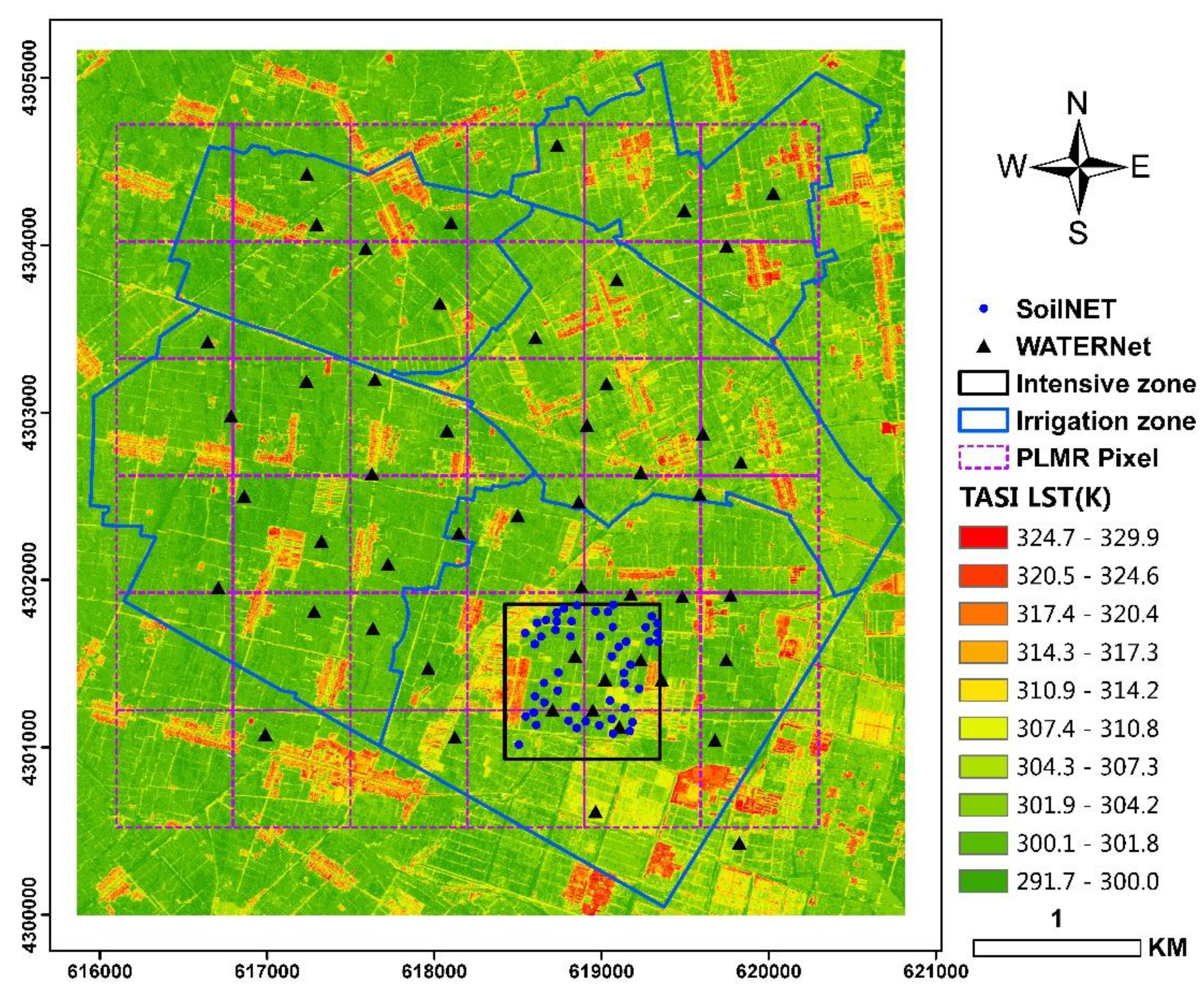
2. Study Area and Data Description
3. Methods
3.1. Upscaling with Spatio-Temporal Regression Block Kriging
3.1.1. Spatio-Temporal Random Field Model
3.1.2. The Trend Component
3.1.3. The Residual Component
3.1.4. Spatio-Temporal Regression Block Kriging
3.2. Accuracy Assessment
4. Results
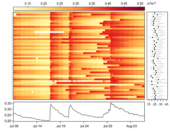
4.1. Data Summary


| Date | Time Duration | Min | Max | Mean | SD | |
|---|---|---|---|---|---|---|
| 10 July 2012 | 9:00–15:00 | WATERNET | 0.198 | 0.339 | 0.256 | 0.033 |
| SoilNET | 0.221 | 0.289 | 0.252 | 0.027 | ||
| 2 August 2012 | 9:00–15:00 | WATERNET | 0.160 | 0.369 | 0.274 | 0.042 |
| SoilNET | 0.237 | 0.312 | 0.278 | 0.034 |
4.2. Regression Modeling of Spatial Trends
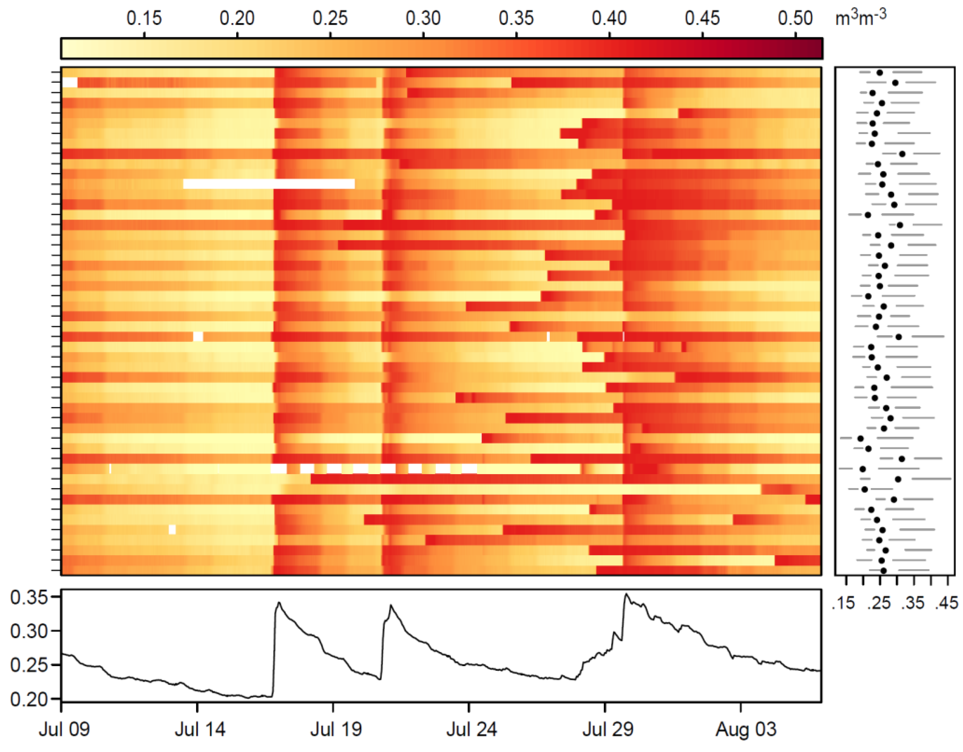
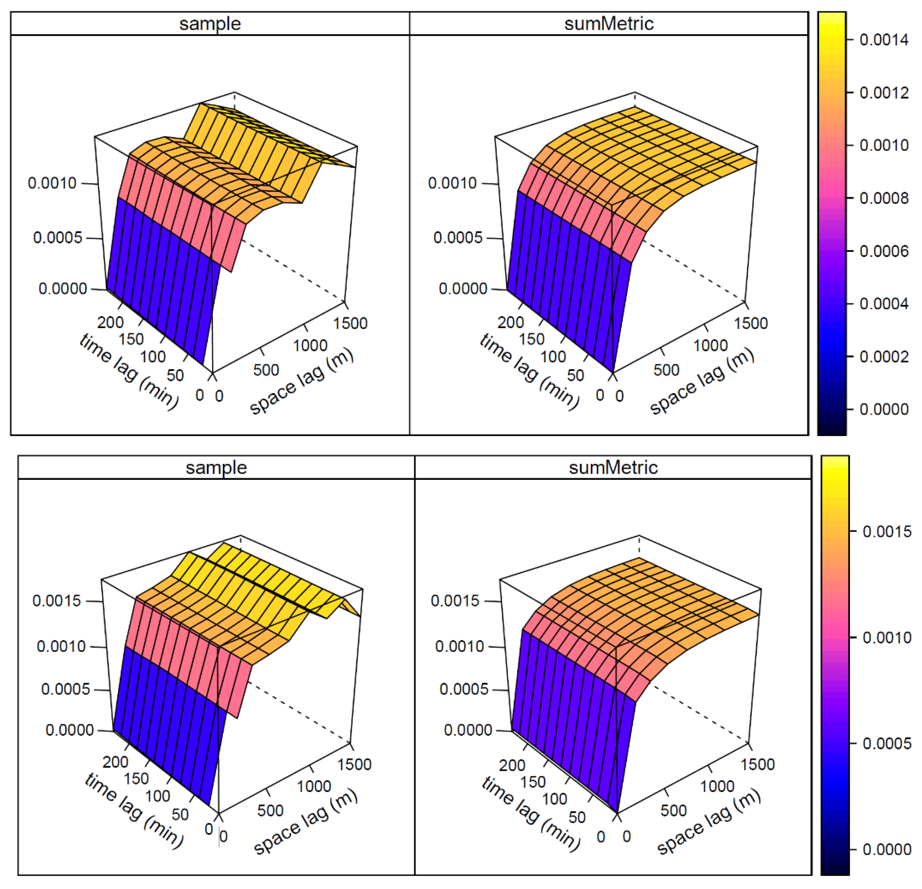
4.3. Variogram Analysis of the Residuals

| Date | Component | Model | Nugget | Sill | Range | Anisotropy |
|---|---|---|---|---|---|---|
| 10 July | Spatial | Exponential | 0 | 0.00098 | 201.1 m | |
| Temporal | Nugget | 0 | 0 | 0 min | ||
| Spatio-temporal | Exponential | 0 | 0.00029 | 35.0 m | 1.56 m/min | |
| 2 August | Spatial | Exponential | 0 | 0.00079 | 265.3 m | |
| Temporal | Nugget | 0 | 0.000012 | 10.0 min | ||
| Spatio-temporal | Exponential | 0 | 0.00068 | 24.0 m | 1.79 m/min |
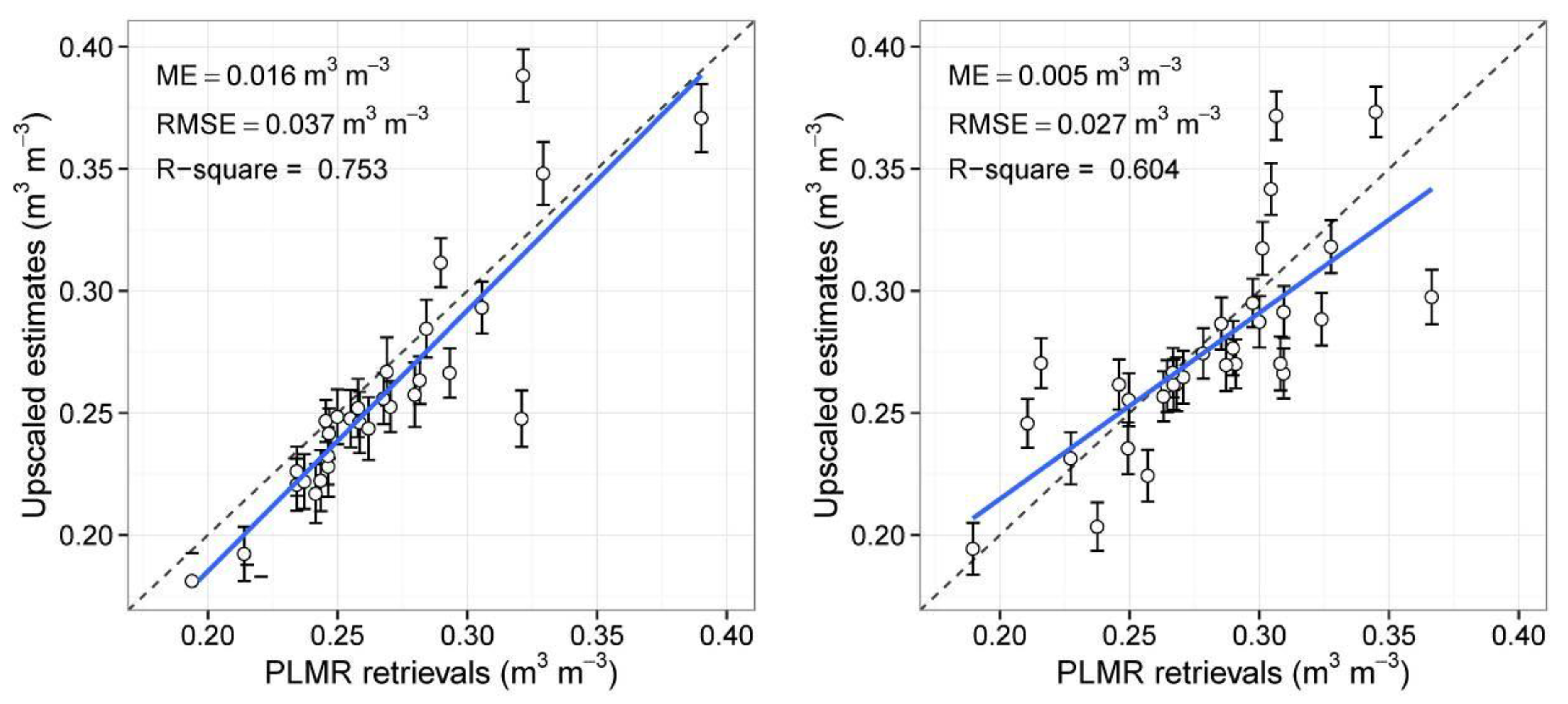
4.4. Accuracy Assessment
| Upscaling Error (m3·m−3) | |||
|---|---|---|---|
| BK | STOBK | STRBK | |
| 10 July | 0.0016 | 0.0014 | 0.0013 |
| 2 August | 0.0017 | 0.0017 | 0.0016 |

5. Discussion
6. Conclusions
Acknowledgments
Author Contributions
Conflicts of Interest
References
- Vereecken, H.; Huisman, J.A.; Bogena, H.; Vanderborght, J.; Vrugt, J.A.; Hopmans, J.W. On the value of soil moisture measurements in vadose zone hydrology: A review. Water Resour. Res. 2008, 44. [Google Scholar] [CrossRef]
- Brocca, L.; Tullo, T.; Melone, F.; Moramarco, T.; Morbidelli, R. Catchment scale soil moisture spatial-temporal variability. J. Hydrol. 2012, 422, 63–75. [Google Scholar] [CrossRef]
- Li, X. Characterization, controlling, and reduction of uncertainties in the modeling and observation of land-surface systems. Sci. China Earth Sci. 2014, 57, 80–87. [Google Scholar] [CrossRef]
- Crow, W.T.; Berg, A.A.; Cosh, M.H.; Loew, A.; Mohanty, B.P.; Panciera, R.; de Rosnay, P.; Ryu, D.; Walker, J.P. Upscaling sparse ground-based soil moisture observations for the validation of coarse-resolution satellite soil moisture products. Rev. Geophys. 2012, 50. [Google Scholar] [CrossRef]
- Jackson, T.J.; Cosh, M.H.; Bindlish, R.; Starks, P.J.; Bosch, D.D.; Seyfried, M.; Goodrich, D.C.; Moran, M.S.; Du, J.Y. Validation of advanced microwave scanning radiometer soil moisture products. IEEE Trans. Geosci. Remote Sens. 2010, 48, 4256–4272. [Google Scholar] [CrossRef]
- Anguela, T.P.; Zribi, M.; Baghdadi, N.; Loumagne, C. Analysis of local variation of soil surface parameters with TerraSAR-X radar data over bare agricultural fields. IEEE Trans. Geosci. Remote Sens. 2010, 48, 874–881. [Google Scholar] [CrossRef] [Green Version]
- Albergel, C.; de Rosnay, P.; Gruhier, C.; Munoz-Sabater, J.; Hasenauer, S.; Isaksen, L.; Kerr, Y.; Wagner, W. Evaluation of remotely sensed and modelled soil moisture products using global ground-based in situ observations. Remote Sens. Environ. 2012, 118, 215–226. [Google Scholar] [CrossRef]
- Qin, J.; Yang, K.; Lu, N.; Chen, Y.Y.; Zhao, L.; Han, M.L. Spatial upscaling of in-situ soil moisture measurements based on MODIS-derived apparent thermal inertia. Remote Sens. Environ. 2013, 138, 1–9. [Google Scholar] [CrossRef]
- Pratola, C.; Barrett, B.; Gruber, A.; Kiely, G.; Dwyer, E. Evaluation of a global soil moisture product from finer spatial resolution SAR data and ground measurements at Irish sites. Remote Sens. 2014, 6, 8190–8219. [Google Scholar] [CrossRef]
- Vereecken, H.; Kasteel, R.; Vanderborght, J.; Harter, T. Upscaling hydraulic properties and soil water flow processes in heterogeneous soils: A review. Vadose Zone J. 2007, 6, 1–28. [Google Scholar] [CrossRef]
- Cressie, N.A.C. Statistics for Spatial Data; Revised ed.; Wiley: New York, NY, USA, 1993; p. 928. [Google Scholar]
- De Rosnay, P.; Gruhier, C.; Timouk, F.; Baup, F.; Mougin, E.; Hiernaux, P.; Kergoat, L.; LeDantec, V. Multi-scale soil moisture measurements at the Gourma meso-scale site in Mali. J. Hydrol. 2009, 375, 241–252. [Google Scholar] [CrossRef]
- Crow, W.T.; Ryu, D.; Famiglietti, J.S. Upscaling of field-scale soil moisture measurements using distributed land surface modeling. Adv. Water Resour. 2005, 28, 1–14. [Google Scholar] [CrossRef]
- Li, X.; Cheng, G.D.; Liu, S.M.; Xiao, Q.; Ma, M.G.; Jin, R.; Che, T.; Liu, Q.H.; Wang, W.Z.; Qi, Y.; et al. Heihe watershed allied telemetry experimental research (HiWATER): Scientific objectives and experimental design. Bull. Am. Meteorol. Soc. 2013, 94, 1145–1160. [Google Scholar] [CrossRef]
- Jin, R.; Li, D. HiWATER: Dataset of Retrieved Soil Moisture Products Using PLMR Brightness Temperatures in the Middle Reaches of the Heihe River Basin. Available online: http://card.westgis.ac.cn/service/pdf/uuid/e48170e3-b4e6-4d75-80f6-39b4abddc862 (accessed on 1 July 2014).
- Hasan, S.; Montzka, C.; Rudiger, C.; Al, M.; Bogena, H.R.; Vereecken, H. Soil moisture retrieval from airborne L-band passive microwave using high resolution multispectral data. ISPRS J. Photogramm. 2014, 91, 59–71. [Google Scholar] [CrossRef]
- Li, D.; Jin, R.; Che, T.; Walker, J.; Gao, Y.; Ye, N.; Wang, S. Soil moisture retrieval from airborne PLMR and MODIS products in the Zhangye oasis of middle stream of Heihe River Basin, China. Adv. Earth Sci. 2014, 29, 259–305. [Google Scholar]
- Jin, R.; Li, X.; Yan, B.P.; Li, X.H.; Luo, W.M.; Ma, M.G.; Guo, J.W.; Kang, J.; Zhu, Z.L.; Zhao, S.J. A nested ecohydrological wireless sensor network for capturing the surface heterogeneity in the midstream areas of the Heihe River Basin, China. IEEE Geosci. Remote Sens. Lett. 2014, 11, 2015–2019. [Google Scholar] [CrossRef]
- Wang, J.H.; Ge, Y.; Song, Y.Z.; Li, X. A geostatistical approach to upscale soil moisture with unequal precision observations. IEEE Geosci. Remote Sens. Lett. 2014, 11, 2125–2129. [Google Scholar] [CrossRef]
- Qu, W.; Bogena, H.R.; Huisman, J.A.; Vereecken, H. Calibration of a novel low-cost soil water content sensor based on a ring oscillator. Vadose Zone J. 2013, 12. [Google Scholar] [CrossRef]
- Bogena, H.R.; Herbst, M.; Huisman, J.A.; Rosenbaum, U.; Weuthen, A.; Vereecken, H. Potential of wireless sensor networks for measuring soil water content variability. Vadose Zone J. 2010, 9, 1002–1013. [Google Scholar] [CrossRef]
- Ge, Y.; Liang, Y.; Wang, J.; Zhao, Q.; Liu, S. Upscaling sensible heat fluxes with area-to-area regression kriging. IEEE Geosci. Remote Sens. Lett. 2015, 12, 656–660. [Google Scholar] [CrossRef]
- Kilibarda, M.; Hengl, T.; Heuvelink, G.B.M.; Gräler, B.; Pebesma, E.; Perčec Tadić, M.; Bajat, B. Spatio-temporal interpolation of daily temperatures for global land areas at 1 km resolution. J. Geophys. Res. Atmos. 2014, 119, 2294–2313. [Google Scholar] [CrossRef]
- Hengl, T.; Heuvelink, G.B.M.; Tadic, M.P.; Pebesma, E.J. Spatio-Temporal prediction of daily temperatures using time-series of MODIS LST images. Theor. Appl. Climatol. 2012, 107, 265–277. [Google Scholar] [CrossRef]
- Heuvelink, G.B.M.; Griffith, D.A. Space–time geostatistics for geography: A case study of radiation monitoring across parts of Germany. Geogr. Anal. 2010, 42, 161–179. [Google Scholar] [CrossRef]
- Cressie, N.A.C.; Wikle, C.K. Statistics for Spatio-Temporal Data; Wiley: Hoboken, NJ, USA, 2011. [Google Scholar]
- De Iaco, S. Space-Time correlation analysis: A comparative study. J. Appl. Stat. 2010, 37, 1027–1041. [Google Scholar] [CrossRef]
- Stein, M.L. Space-time covariance functions. J. Am. Stat. Assoc. 2005, 100, 310–321. [Google Scholar] [CrossRef]
- Snepvangers, J.J.J.C.; Heuvelink, G.B.M.; Huisman, J.A. Soil water content interpolation using spatio-temporal kriging with external drift. Geoderma 2003, 112, 253–271. [Google Scholar] [CrossRef]
- Pebesma, E.J. Multivariable geostatistics in S: The gstat package. Computat. Geosci. 2004, 30, 683–691. [Google Scholar] [CrossRef]
- Pebesma, E. Spacetime: spatio-temporal data in R. J. Stat. Softw. 2012, 51, 1–30. [Google Scholar]
- R Development Core Team. R: A Language and Environment for Statistical Computing; R Foundation for Statistical Computing: Vienna, Austria, 2014. [Google Scholar]
- Peng, R. A method for visualizing multivariate time series data. J. Stat. Softw. 2008, 25, 1–17. [Google Scholar]
- Zhu, Z.; Tan, L.; Gao, S.; Jiao, Q. Observation on soil moisture of irrigation cropland by cosmic-ray probe. IEEE Geosci. Remote Sens. Lett. 2015, 12, 472–476. [Google Scholar] [CrossRef]
- Qin, J.; Zhao, L.; Chen, Y.; Yang, K.; Yang, Y.; Chen, Z.; Lu, H. Inter-comparison of spatial upscaling methods for evaluation of satellite-based soil moisture. J. Hydrol. 2015, 523, 170–178. [Google Scholar] [CrossRef]
© 2015 by the authors; licensee MDPI, Basel, Switzerland. This article is an open access article distributed under the terms and conditions of the Creative Commons Attribution license (http://creativecommons.org/licenses/by/4.0/).
Share and Cite
Wang, J.; Ge, Y.; Heuvelink, G.B.M.; Zhou, C. Upscaling In Situ Soil Moisture Observations to Pixel Averages with Spatio-Temporal Geostatistics. Remote Sens. 2015, 7, 11372-11388. https://doi.org/10.3390/rs70911372
Wang J, Ge Y, Heuvelink GBM, Zhou C. Upscaling In Situ Soil Moisture Observations to Pixel Averages with Spatio-Temporal Geostatistics. Remote Sensing. 2015; 7(9):11372-11388. https://doi.org/10.3390/rs70911372
Chicago/Turabian StyleWang, Jianghao, Yong Ge, Gerard B. M. Heuvelink, and Chenghu Zhou. 2015. "Upscaling In Situ Soil Moisture Observations to Pixel Averages with Spatio-Temporal Geostatistics" Remote Sensing 7, no. 9: 11372-11388. https://doi.org/10.3390/rs70911372