Article

Multisensoral Topsoil Mapping in the Semiarid Lake Manyara Region, Northern Tanzania

by
Felix Bachofer
1,*,
Geraldine Quénéhervé
1,
Volker Hochschild
1 and
Michael Maerker
2,3
1
Institute of Geography, University of Tuebingen, Ruemelinstr. 19-23, 72070 Tuebingen, Germany
2
Heidelberg Academy of Sciences and Humanities, Ruemelinstr. 19-23, 72070 Tuebingen, Germany
3
Earth Science Department, University of Florence, Via G. La Pira, 50121 Florence, Italy
*
Author to whom correspondence should be addressed.
Remote Sens. 2015, 7(8), 9563-9586; https://doi.org/10.3390/rs70809563
Submission received: 21 May 2015 / Revised: 19 July 2015 / Accepted: 20 July 2015 / Published: 28 July 2015

Abstract

:
This study pursues the mapping of the distribution of topsoils and surface substrates of the Lake Manyara area of northern Tanzania. The nine soil and lithological target classes were selected through fieldwork and laboratory analysis of soil samples. High-resolution WorldView-2 data, TerraSAR-X intensity data, medium-resolution ASTER spectral bands and indices, as well as ENVISAT ASAR intensity and SRTM-X-derived topographic parameters served as input features. Objects were derived from image segmentation. The classification of the image objects was conducted applying a nonlinear support vector machine approach. With the recursive feature elimination approach, the most input-relevant features for separating the target classes were selected. Despite multiple target classes, an overall accuracy of 71.9% was achieved. Inaccuracies occurred between classes with high CaCO3 content and between classes of silica-rich substrates. The incorporation of different input feature datasets improved the classification accuracy. An in-depth interpretation of the classification result was conducted with three soil profile transects.

Graphical Abstract

1. Introduction

The spatial distribution of soils and lithology provides essential input information for different scientific and economic applications, including landscape reconstruction [1], digital soil mapping (DSM) and mineral exploration for agricultural [2] or mining applications [3]. Though the soil must be considered as a three dimensional medium, a wide range of remote sensing sensors provide useful information in assessing various details of the mineral composition and other physical and/or chemical properties of the uppermost parts of the soils, as well as for spatially contiguous areas [4,5,6]. The topsoil is generally the most relevant part of the soil, considering food production, degradation and soil management [7]. Although the definition of topsoil varies in different soil taxonomies [7,8,9,10], the uppermost part of the soil belongs to the topsoil. The topsoil thickness is related to local conditions of pedogenesis, erosion and deposition processes. Normally, topsoil is characterized by a thickness of 10–30 cm [7,8]. In this study, we regard the soil surface properties as topsoil/lithology proxy. We hypothesize that the analysis of physical-chemical properties, the collection of field reference data and the remote sensing analysis of the upper surface strata yield valuable information about the topsoil and/or lithologic characteristics. Moreover, the topographic position and geomorphological processes also influence the topsoil characteristics and, hence, should be included in a comprehensive analysis of the spatial distribution of topsoils.
The surface reflectance of the mineral composition of a surface, which is received by a multi- or hyper-spectral sensor, is influenced by soil organic matter, moisture content, as well as texture and surface roughness [11]. Backscatter signals from Synthetic Aperture Radar (SAR) sensors of different wavelengths are dependent on the surface roughness and are sensitive to the dielectric properties of soils [12,13,14]. Soil mapping using remote sensing data show limitations due to the complex physical and chemical nature of soils. Remotely derived datasets can characterize the surface (optical remote sensing systems) or the uppermost part of soils (SAR systems) [5,15]. Since soils are complex three-dimensional structures, the surface characteristics may not represent the underlying layers of soil. The remote sensing signal may also be a product of different soil surface properties. This effect will increase with a lower spatial resolution of the datasets. Very high-resolution sensors, like WorldView-2 and GeoEye-1, provide a high spatial differentiation. On the other hand, lower spatial resolution sensors, like the Landsat series or ASTER, provide a better spectral coverage, especially in the mid-infrared region, which is important for mineral mapping purposes [5,16]. Vegetation cover is another important factor to consider. Already sparse vegetation cover may influence the identification of soil attributes using remote sensing methods [17,18]. Spectral indices from multi- or hyper-spectral remote sensing images are effective tools for the classification and evaluation of photosynthetic vegetation activity. Vegetation indices (VI), like the Normalized Difference Vegetation Index (NDVI), utilize the difference of absorption and reflection in the spectral wavelengths of the red (0.625–0.74 µm) and near-infrared (IR; 0.74–1 µm) [19]. Dead materials in grasslands blur VI, making it hard to distinguish between dead materials and some other land cover [20]. This is especially a problem in arid and semiarid regions, due to relatively long dry periods. A strategy to resolve these problems consists of long-term monitoring via remote sensing and collection of ground information [21,22].
A wide range of studies proved the applicability of techniques using remote sensing data for topsoil mapping. In the following, some of them are described. Landsat 5 TM imagery was used to detect basalt outcrops for supporting soil mapping, applying reflectance values, band ratios and indices [23]. Landsat 7 ETM+ data were used to determine surface soil properties with the help of laboratory-analyzed surface soil samples [24]. The ASTER multispectral bands and derived indices and ratios were often utilized for lithological mapping [25,26,27,28]. ASTER data were also used to identify mineral components in tropical soils using reflectance spectroscopy signatures from soil samples [29].
Various studies include additional variables, especially in geostatistical approaches of the spatial soil distribution [5]. Topographical features, in particular, provide information on the terrain and, hence, on soil formation processes [30]. Mulder et al. [31] used ASTER data and derivatives, as well as elevation as topographical proxy for DSM. Hahn and Gloaguen [32] compared different input variable combinations of ASTER-derived land use, geology, topographical parameters and others to estimate soil distribution by support vector machines (SVM). Rossel and Chen [33] used Landsat data and derivatives, topographical derivatives, climate parameters, as well as soil, geological and radiometric maps and spectrometry results from soil samples to determine the surface soil properties for Australia. Selige et al. [34] found out that soil organic matter and soil texture of topsoil correlate with the spectral properties of a hyperspectral sensor. They were also able to model the distribution of sand, clay, organic carbon (Corg) and nitrogen. SAR backscatter intensity information from X-, C- and L-band sensors proved to be sensitive for soil moisture differences, surface roughness and, to some extent, also to soil texture [13,14,35,36,37,38,39,40,41]. Hengl et al. [42] applied an automated random forest approach to map soil properties of Africa with DEM-based landforms parameters and MODIS data at a spatial resolution of 250 m for the Africa Soil Information Service (AfSIS) project. A comprehensive overview about remote sensing in soil mapping is provided by Mulder et al. [5] and with a special focus on Africa by Dewitte et al. [6].
The lithologies and the soils of the Lake Manyara basin have complex genetic origins. The Proterozoic gneissic basement, tectonic and volcanic processes, as well as the (paleo-)hydrological processes and the sedimentation of the paleolake Manyara influence soil formation. This results in a small-scale distribution and fuzzy transitions of today’s soils, topsoils and outcropping lithology, which cannot be depicted by the available soil map for the region with a scale of 1:2,000,000 [43]. Consequently, the categorization of soils is a complex process due to their three-dimensional nature. Hence, remotely-sensed surface features yield auxiliary information of topsoil characteristics and their distribution. Combined with topographic information, the analysis results in valuable information that allows also a rough identification of soil types.
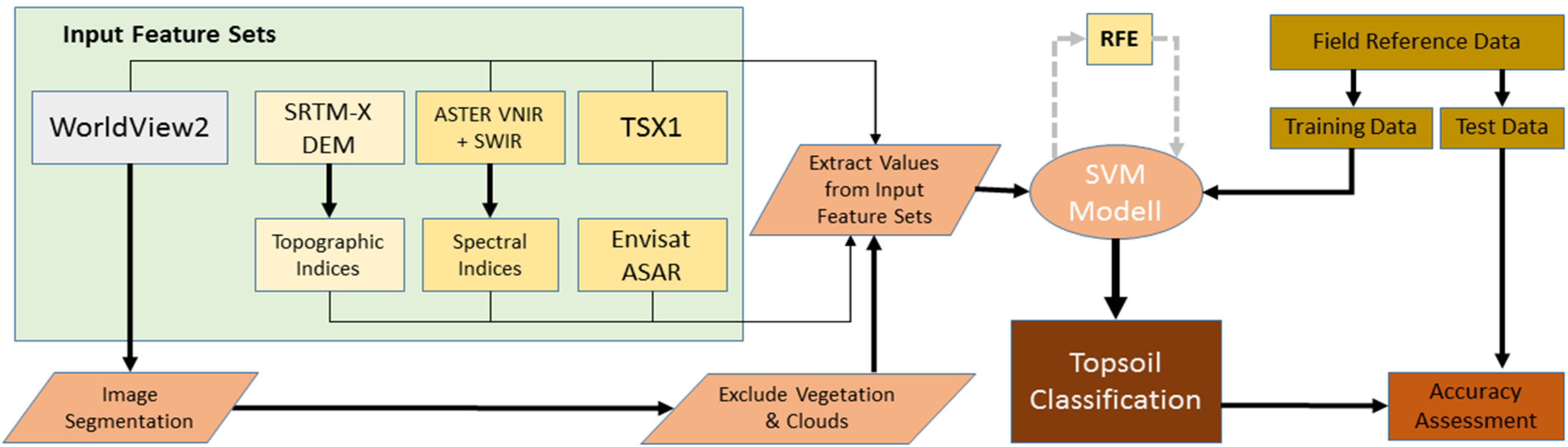
The aim of this study is to map the distribution of the topsoil and surface substrate characteristics using multispectral, topographical and SAR input data. The laboratory analysis of surface samples provides soil properties used to categorize and characterize the topsoils and surface substrates. In order to improve the topsoil classification, we followed a multiscale approach using: (i) image object segments from a high-resolution WorldView-2 scene; (ii) low-resolution ASTER multispectral data and indices; (iii) X- and C-band SAR backscatter; as well as (iv) topographical derivatives. We compare and discuss the final mapping results with soil catenae covering characteristic transects of the study area.
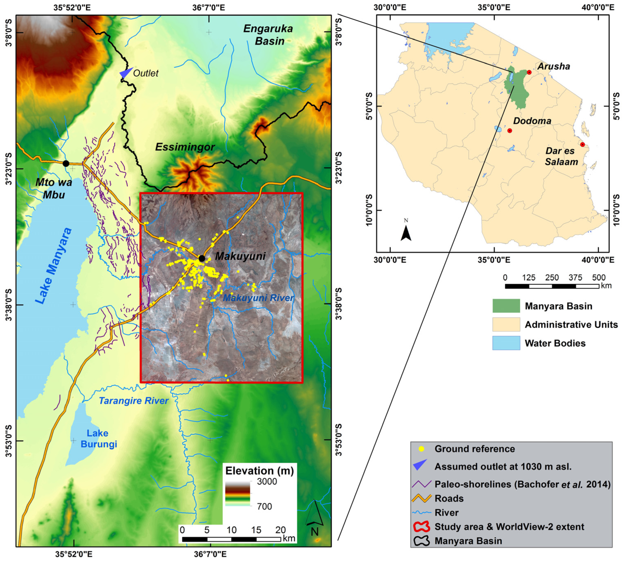
2. Study Area

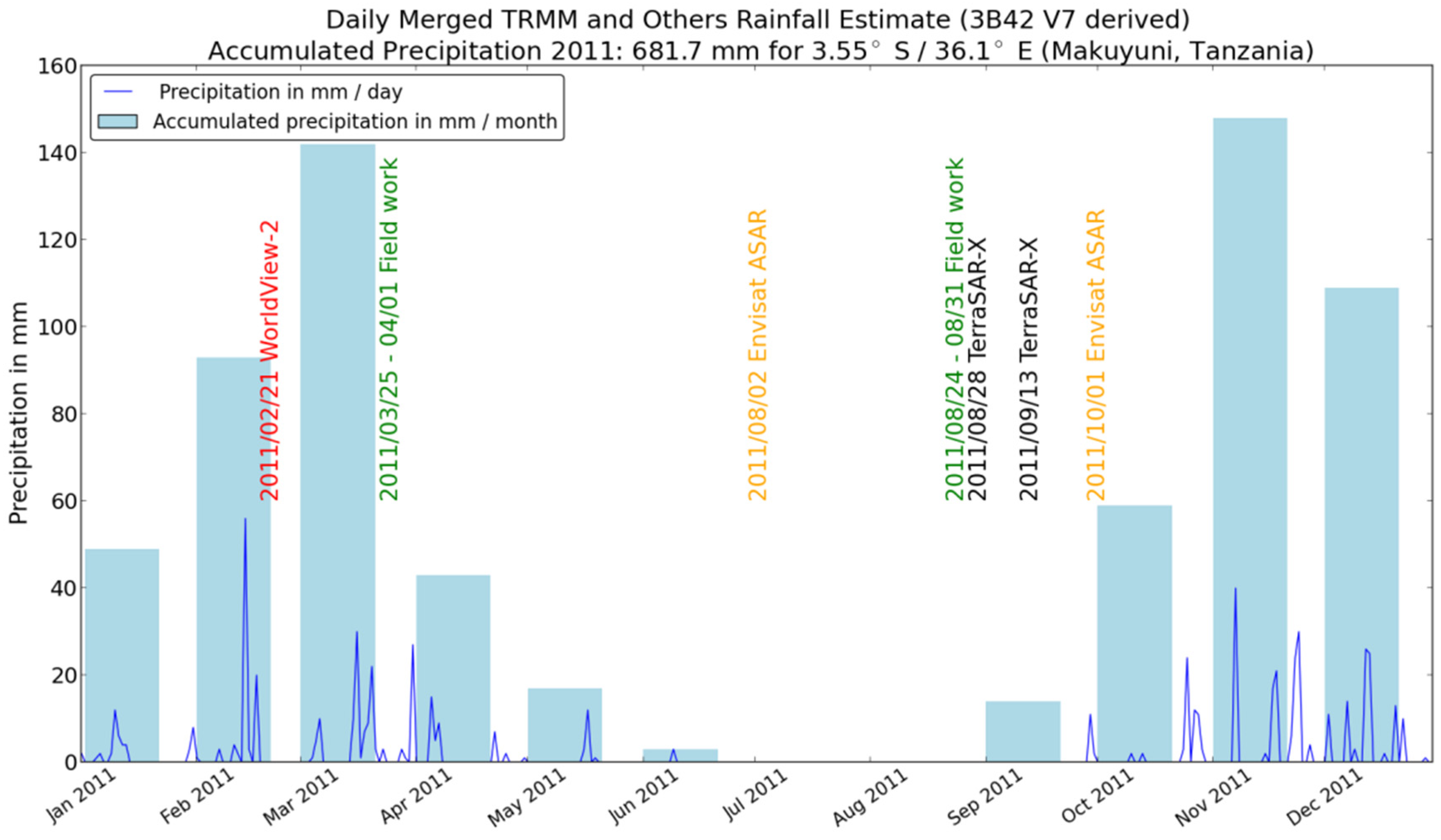
The study area is located within the East African Rift System of northern Tanzania; in the surroundings of the Makuyuni village. The area is drained towards the west by the Makuyuni River disemboguing into the endorheic Lake Manyara Basin (Figure 1). The precipitation calculations from the daily Rainfall Estimate Product 3B42 (V7) of the Tropical Rainfall Measurement Mission (TRMM) show a bimodal rainfall pattern for the years 2000–2013 [44]. For this period, the average annual precipitation of 651 mm is mainly caused by two wet seasons. One occurs between November and January and a second between March and May [45]. This results in a sparsely-vegetated semiarid environment dominated by bushy grassland. The study area is also characterized by a variety of degradation processes due to long dry periods and short, but intensive rainfall events, as well as contributing anthropological factors, like overgrazing [46].
Figure 1. Study area.
Remotesensing 07 09563 g001
The lithology of the study area is very complex, because different lithological units interleave here. The underlying basement of the Masai Plateau is formed of Proterozoic intermediate quartzite and gneisses and is exposed by tectonic faults [47]. Explosive volcanism, especially from the volcano Essimingor, and faulting associated with the rifting of the basin produced alkaline lavas, like alkali basalt, phonolite, nephelinite and tuffs. The volcano Ol Doinyo Lengai (90 km north of the study area) has a carbonate volcanism, and its carbonate tephra deposits are widespread [47,48,49]. Lacustrine and fluvially deposited sediments can be found 140 m above today’s level of Lake Manyara. The so-called Manyara Beds crop out where the Makuyuni River and gully system incise into the lacustrine and terrestrial deposits. The lower member of the Manyara Beds is of lacustrine origin and is composed mainly of mudstones, siltstones, diatomites, marls and tuff that have been deposited in a reducing environment. These sediments have an age of approximately 1.03–0.633 Ma. A tephra layer, which was dated to 0.633 Ma, marks the transition of the younger upper member of the Manyara Beds [50,51,52].

3. Input Data and Pre-Processing

Multiscale remote sensing data and their derivatives, as well as topographic indices delineated from a Shuttle Radar Topography Mission (SRTM) DEM served as input information for the analysis. All image datasets were co-registered to ensure complementary datasets.

3.1. WorldView-2

WorldView-2 is a commercial multispectral sensor, which was launched in October 2009. It has a very high geometrical resolution for its’ eight multispectral bands (MS) at 1.85 m ground resolution and for the panchromatic band of 0.46 m at nadir [53]. The scene was acquired on 21 February 2011 (Table 1); following the winter wet season and a strong precipitation event mid-February (Figure 2).
Table 1. Optical remote sensing sensors. MS: multispectral.
SensorDateTime (UTC)No. of BandsWavelengthSpatial Resolution
WorldView-221 February 201108:2280.40–1.04 µm1.85 m (MS)
ASTER-VNIR23 August 200608:0730.52–0.86 µm15 m
ASTER-SWIR23 August 200608:0761.60–2.43 µm30 m
Figure 2. Precipitation, fieldwork and remote sensing data of the year 2011.
Remotesensing 07 09563 g002

3.2. ASTER Bands and Indices

The Advanced Spaceborne Thermal Emission and Reflection Radiometer (ASTER) consists of three subsystems with a spectral coverage in the visible-near infrared (VNIR), the shortwave infrared (SWIR) and the thermal infrared (TIR) wavelength regions (Table 1). ASTER was launched onboard NASA’s TERRA spacecraft in December 1999. The spectral resolution was mainly designed for vegetation, soil and mineral mapping [54]. An ASTER L1B scene was obtained on 23 August 2006 after a long dry season. Because of the cross-detector leakage between the SWIR bands, crosstalk correction was applied using a correction tool from the Earth Remote Sensing Data Applications Centre (ERSDAC) [55].
The six spectral bands of the SWIR system were selected as input features for the analysis. Spectral indices derived from the ASTER VNIR and SWIR bands were also included as input parameters (Table 2). The purpose of these indices is a relative amplification of selective absorption and reflection features, which are caused by different surface materials at distinct wavelengths. They help to detect different mineral compositions, but also to emphasize the spectral differences of target objects. The indices listed in Table 2 are based on a comprehensive literature review.
Table 2. Spectral indices of ASTER VNIR and SWIR bands.
Index with Literature ReferenceFormulaIndex with Literature ReferenceFormula
Alunite/Kaolinite/Pyrophyllite Index [25](4 + 6)/5AlOH Group Index [56](5/7)
Alteration/Laterite Index [57](4/5)Alunite Index [28](7/5) × (7/8)
Calcite Index [28](6/8) × (9/8)Carbonate/Chlorite/Epidot Index [25](7 + 9)/8
Clay—1 Index [25](5 + 7)/6Clay—2 Index [57](5 × 7)/(6 × 6)
Dolomite Index [25](6 + 8)/7Ferric Iron (Fe3+) Index [25](2/1)
Ferric Oxide Index [56](4/3)Ferrous Iron (Fe2+)—1 Index [26](1/2)
Ferrous Iron (Fe2+)—2 Index [26](5/3) + (1/2)Ferrous Iron/Silicates Index [56](5/4)
Kaolinite Index [28](4/5) × (8/6)Kaolin Group Index [56](6/5)
Kaolinitic Index [58](7/5)MgOH—1 Index [58](6 + 9)/8
MgOH—2 Index [56](7/8)Muscovite Index [58](7/6)
OH Bearing Altered Minerals—1 Index [28](7/6) × (4/6)OH Bearing Altered Minerals—2 Index [59](4 × 7/6/6)
OH Bearing Altered Minerals—3 Index [59](4 × 7/5/5)Opaque Index [56](1/4)
Phengitic Index [58](5/6)Relative Band Depth 6 (RBD6) [26](4 + 7)/(6 ×2)
Relative Band Depth 8 (RBD8) [26](7 + 9)/(8 × 2)

3.3. Topographic Indices

During the Shuttle Radar Topography Mission (SRTM) in the year 2000, X-band data were acquired, which provided a DEM with 25 m ground resolution. The SRTM-X dataset has no full coverage worldwide; however, one track covers the study area. The DEM was projected to the Earth Gravitational Model (EGM96) vertical datum. The short wave X-band-derived DEM resulted in good elevation accuracy [60], but also yielded small-scale noise at the surface. To reduce this effect while preserving the topography, we applied a multidirectional Lee filter [61]. The DEM was used to calculate different topographic indices, which characterize the topographic position of the topsoils in the study area (Table 3).
Table 3. Topographic indices.
Index with Literature ReferenceIndex with Literature Reference
Elevation (height above sea level; a.s.l) [62]Geomorphons [63]
Slope Length Factor [64]Morphometric Protection Index [51]
Multiresolution Index of Ridge Top Flatness (MRRTF) [65]Multiresolution Index of Valley Bottom Flatness [65]
Negative Openness [66]Positive Openness [51]
Plan Curvature [67,68]Slope [69]
Stream Power Index [64]Terrain Classification Index for Lowlands [70]
Terrain Ruggedness Index [71]Topographic Position Index [72]
Topographic Wetness Index [73]Vertical Distance to Channel Network [74]

3.4. SAR Data

We acquired two TerraSAR-X (TSX1) (~9.65 GHz; X-band) StripMap and two Envisat ASAR (~5.331 GHz; C-band) scenes for different dates (Table 4). Precise orbits were applied to the ASAR scenes. All SAR scenes were calibrated and radiometrically corrected for topographic effects to gamma naught (γ) using the local incident angle derived from the SRTM-X DEM. The scenes were terrain corrected, and speckle effects were reduced by applying a Lee filter [61]. The two TSX1 scenes were mosaicked to a single dataset in order to cover the whole study area. The images were acquired in the dry season (Table 4; Figure 2), to minimize the influence of soil moisture on the backscatter intensity signal [36,37,38,75].
Table 4. SAR images. TSX1, TerraSAR-X.
SensorModeDateTime (UTC)OrbitIncident Angle Range (Degrees)PolarizationSpatial Resolution
Envisat ASARAP2 August 201107:22Descending31.0–36.3°VV/VH30 m
Envisat ASARAP1 October 201107:22Descending31.0–36.3°VV/VH30 m
TSX1StripMap28 August 201115:46Ascending26.3° (scene center)HH3 m
TSX1StripMap13 September 201115:54Ascending44.4° (scene center)HH3 m

3.5. Field Reference Data, Laboratory Analysis and Target Classes

During six field campaigns from 2010 to 2014, 602 reference sites were visited within the study area, including fieldwork conducted one month after the acquisition of the WV-2 scene. Because the southern and eastern parts of the study area are remote and partly inaccessible, we decided on a random clustered sampling strategy (Figure 1). The landscape is considered as stable and the mineral components as conservative in relation to the resolution of the input data. The collected parameters consist of: texture, calcium carbonate (CaCO3) content (with hydrochloride acid), soil color, visible mineral components of surface substrates, vegetation cover, topographic position, GPS and photo references. The reference points serve as training and test data for the SVM analysis.
The categorization of soils and topsoils is a complex process. In addition to the description of field reference points, we also conducted laboratory analyses for a better understanding and for the target class selection. From 27 reference locations, surface substrate samples (0–2 cm) were collected and physical and chemical analyses conducted (Table 5). Soil samples were air-dried and sieved (<2 mm). Texture was analyzed with the Bouyoucos hydrometer method after dispersing the samples with 1N sodium hexametaphosphate and represented according to the United States Department of Agriculture (USDA) classification [8]. CaCO3 was measured using the methods proposed in Buurman et al. [76]. Corg was determined using the Springer and Klee method [77]. Available fractions of heavy metals (Fe and Mn) were extracted according to the Lindsay–Norwell procedure [78]. Exchangeable bases (K, Ca, Mg and Na) are analyzed based on the Mehlich 3 method [79]. The field reference collection and the laboratory samples resulted in seven topsoil classes (Table 5), two additional lithological classes (Figure 3) and a class for surface water (Class 1), which includes the Makuyuni River and water reservoirs for cattle farming and irrigation.
Table 5. Laboratory analysis of topsoil samples (meq = milliequivalents; mmol = millimoles).
ClassNumber of topsoil SamplesLaboratory Analysis
Coarse Sand (0.5–2 mm) in g/kgFine/Medium Sand (0.05–0.5 mm) in g/kgSilt (0.002– 0.05 mm) in g/kgClay (<0.002 mm) in g/kgCalcium Carbonate CaCO3 in g/kgOrganic Carbon (Corg) in g/kgIron (Fe) in mg/kgManganese (Mn) in mg/kgAluminium (Al) in mg/kgCalcium Cation (Ca2+) in meq/100 gMagnesium Cation (Mg2+) in meq/100 gSodium Cation (Na+) in meq/100 gPotassium Cation (K+) in meq/100 gChlorides (Cl) in mg/kgWater soluble Sulfate (SO4) in mmol/kg
24117.25503.75166.00279.50128.002.754.017.600.287.534.404.870.9791.378.87
3574.80344.80143.80367.60115.6020.626.5420.720.1718.885.096.771.8059.9045.78
4492.60216.00416.60274.8026.7914.619.6436.800.2124.136.076.311.8813.868.54
5183.00280.00134.00475.002.009.809.1720.140.2222.463.706.101.087.207.80
67134.86327.57317.14220.4312.2915.479.0949.800.2514.984.665.812.2410.016.94
74384.00374.50156.75120.750.7510.055.7040.480.254.791.540.261.4618.6810.20
8241.00235.50101.00278.5025.0015.8526.4076.040.4718.257.770.212.4414.258.90
Figure 3. Target classes identified by field surveys and laboratory analysis (Class 1 = water).
Remotesensing 07 09563 g003
“Carbonate-rich substrate” (Class 2) mostly consists of erosive areas with lacustrine sediments and more than 20% carbonate gravel or concretions. Class 2 appears with the Lower Manyara Beds, associated calcaric Regosols and secondary hardened carbonates. The CaCO3 content is rather high (128 g/kg) and the Corg content relatively low (2.75 g/kg). “Calcaric topsoil” (Class 3) features a high CaCO3 content and a comparatively high clay content. “Dark topsoil” (Class 4) shows the highest silt content, is dark in color (Munsell® color: hue of 7.5 or 10 YR (yellow red); values of ≤3 or lower; chroma of ≤2), has a low CaCO3 content compared to “Class 3” and a low Fe content compared to “Class 8”. It is associated with colluvial and fluvial deposits. “Tuff outcrop” (Class 5) defines distinct outcropping layers of hardened tuff. “Reddish topsoil” (Class 6) has a distinct hue of 5 YR or redder (Munsell® color) and can be distinguished from “Class 3” by a low CaCO3 content, from “Class 4” by color and texture, from “Class 7” by texture, cations and Fe content and from “Class 8” by Fe and Mn content. “Silica-rich topsoil” (Class 7) is associated with the felsic basement and the high quartz sand and grit content, which is a surface residual due to selective erosion. The hue of the soil is 5–7.5 YR; the color value is 4; and the chroma 6–4 (Munsell® color). The “Topsoil with iron oxides properties” (Class 8) class describes a soil associated with mafic lithology (Class 9) and with a high Fe and Mn content, which makes it clearly distinguishable from “Class 3” and “Class 4”. “Mafic-dominated cover beds” (Class 9) describe outcroppings and weathered mafic (nephelinite, phonolite, basalt) ridges and the Essimingor volcano. “Mafic river beds” (Class 10) are the same material as “Class 9”, but the boulders are hardly weathered, which results in different spectral properties and concentrates within the river beds.
In order to validate and interpret the results of the topsoil and surface substrates’ classification procedure, we conducted three soil catenae consisting of 24 soil profiles with detailed profile descriptions according to the World Reference Base for Soil Resources (WRB) 2014 [80].

4. Methods

The workflow consists of several steps (Figure 4): (I) image segmentation based on the high-resolution WorldView-2 images; (II) vegetation and areas affected by clouds and shadowing effects were excluded from further processing; (III) for each remaining segment, mean values of the input feature sets listed in the previous section (Table 3 and Table 4) were extracted; (IV) an SVM model was built; (V) SVM-recursive feature elimination (RFE) reduced the number of variables before classifying the segments with the SVM approach; (VI) we compared the results of various input feature set combinations; (VII) accuracy assessment; and (VIII) external validation using soil catenae.
Figure 4. Proposed workflow. RFE, recursive feature elimination.
Remotesensing 07 09563 g004

4.1. Image Object Segmentation

Image objects, which represent contiguous areas in the image, were delineated by multi-resolution segmentation [81]. The segmentation is purely based on the WorldView-2 bands. The reasons for applying an object-oriented approach are reduced processing costs, the possibility to extract values from multiple scales and the option to generate additional object-based input features. The multi-resolution segmentation is a bottom-up approach, which applies region merging beginning with the pixel level [82]. The heterogeneity measurement ƒ (Equation 1), which defines if objects are merged, is controlled by a threshold. If the heterogeneity measure exceeds the threshold, which is determined by the scale parameter, the merging of image objects is terminated. ∆hcolor defines the difference in spectral heterogeneity and ∆hshape the consideration of the smoothness and compactness of the image objects. wcolor and wshape are the according weight measures [82].
ƒ = wcolor × ∆hcolor + wshape × ∆hshape, wcolor ∈ [0, 1,] , wshape ∈ [0, 1,] wcolor + wshape = 1
Roads and buildings were easily identified from the resulting segments by spectral values, shape and spatial relations. Since the image acquisition took place shortly after the winter rainy season, we could verify in the field that, with the exception of some rare occasions, all vegetation cover was photosynthetic active. Therefore, vegetation cover was determined by NDVI thresholding, utilizing a histogram. These three land cover types were excluded from further processing, since they are not the focus of the research objective. This is especially important for the vegetation, because the influence on the spectral response (dead organic materials, as well as photosynthetic vegetation) is considered high [20].
After this pre-selection, 47% of the study area of 1200 km2 was considered as open soil or vegetation-free lithology. Some of the reference points had to be excluded from further analysis, leading to 432 vegetation-free reference points. The 1,005,058 image segments result in an average mapping unit of 550 km2. For these image objects, mean values from the SAR images, ASTER bands and indices, as well as from topographic parameters were extracted. The following additional input features were computed from WV2: (i) standard deviation for all spectral bands; (ii) NDVI [19]; (iii) spectral brightness; and (iv) texture homogeneity measure following Haralick et al. [83].

4.2. Support Vector Machines

The machine learning concept of SVM was developed to solve binary problems in pattern recognition applications. The development and theoretical background is published by Vapnik [84,85], Hearst [86], Burges [87] and Schölkopf and Smola [88]. Remote sensing studies make use of SVM properties, like high computation performance and high classification accuracies with small numbers of training samples [89]. Recent studies used SVM approaches to identify lithological units with remote sensing data [90,91].
The fundamental principle of SVM is the maximization of margins between training samples of two target classes. Not all features of the training dataset are used for this approach; only those samples that are close to the margin. They serve as support vectors, which are used to define the boundaries of the margin. A maximized margin is referred to as the optimal separating hyperplane [87]. To prevent an over-fitting of the hyperplane caused by outliers in the training dataset, a “soft margin” approach was introduced [92]. This approach uses a cost parameter (C), which determines a penalty for the support vectors. Low C values indicate a stronger generalization of the model; high values provide more influence for single input features [93].
For this study, we utilized a support vector classifier (C-SVC) provided by the Library for Support Vector Machines (LIBSVM) [94]. C-SVC works as a “one-against-one” classifier that discriminates between two target classes. A multi-class approach is solved by constructing multiple target value pairs. In some cases, including soil-related issues, it is hardly possible to separate the target classes in a single input space with a linear function [32]. SVMs therefore project the input features in an n-dimensional feature space. To avoid the computational effort of projecting all input features into a multi-dimensional feature space, kernels can be used to calculate their dot product in the feature space. Various kernels can be applied with SVMs. In this study, a radial basis kernel function (RBF) was utilized, which is widely used when a nonlinear distribution of feature values is expected [32,95]. A linear kernel serving as reference was also applied. The width of the RBF, and hence, the influence of a training sample on the adjacent feature space, is controlled by the constant γ. High values indicate a strong influence, whereas low values indicate a weak influence. Thirty percent of the reference samples (130) were randomly selected to serve exclusively as test datasets, and the remaining 70% was used for the training of the SVM model. All input feature sets were scaled to a range of [−1, +1]. For the derivation of the constants C and γ, a grid search was conducted by an iterative cross-validation of the performance of fitting the model to the training data [94].

4.3. Recursive Feature Selection

In order to identify a minimum subset of features that contribute to the discrimination of the target classes, a RFE technique was applied [96]. Many of the spectral and topographical input features carry redundant information. A subset of features provides, in addition to a higher computation performance, the possibility for a better interpretation of the interrelation between the topsoil reference and the spectral and topographic parameters of the datasets explaining the topsoil distribution. RFE is a backward elimination method, which starts with a full set of features and iteratively reduces their number according to their contribution to the classification accuracy [97]. For this, the SVM classifier is trained at each iteration, and a ranking criterion is computed for all features. The feature with the smallest criterion is then removed before the next iteration [98]. SVM-RFE was performed with the e1071 package [99].

5. Results and Discussion

The comparison of different input feature groups shows that all additional input features increase the overall accuracy of the classification (Table 6). The classification of only the spectral bands of WorldView-2 with an RBF-kernel reaches an accuracy of 62.9%. By incorporating more features from the ASTER data, SAR scenes and topographic indices, an overall accuracy of 70.4% was achieved. By conducting the classification with the parameters selected by RFE (Table 7), the highest accuracy of 71.9% was reached. The application of a linear kernel instead of an RBF-kernel led to lower accuracies.
Table 6. Overall accuracies for different input feature groups. RBF, radial basis function.
Input Feature GroupsNo. of Input FeaturesCgOverall Accuracy
WorldView-2 81896.00.062562.9%
WorldView-2 + WV2 derivatives8 + 11185,3630.0000663.7%
WorldView-2 and SAR scenes8 + 5160.062565.2%
WorldView-2 and ASTER bands / indices8 + 33181.020.005564.4%
WorldView-2 and topographic parameters8 + 1665,536.00.0000567.4%
All available parameters732.820.088370.4%
Selection from RFE (linear kernel)241.41-66.6%
Selection from RFE (RBF-kernel)384.000.125071.9%
Table 7. Relevance ranking of RFE selected input features. SD, standard deviation.
RFE RankInput FeatureRFE RankInput FeatureRFE RankInput Feature
1Geomorphons2MRRTF3WV2—Band 3
4Ferric Iron (Fe3+) Index5WV2—Band 16Calcite Index
7AlOH Group Index8WV2—SD Band 39Ferrous Iron 1 Index
10Ferric Oxide Index11RBD812WV2—Band 8
13WV2—Band 414WV2—SD Band 115Alteration/Laterite Index
16ASTER SWIR Band 617Opaque Index18Clay 2 Index
19MgOH 2 Index20WV2—SD Band 421WV2—Band 2
22Kaolinite Index23Terrain Ruggedness Index24TSX1 HH intensity
25Envisat ASAR (1 October 2011 VV)26WV2 NDVI27ASTER SWIR Band 4
28Morphometric Protection Index29WV2—Band 730ASTER SWIR Band 3
31WV2—SD Band 832WV2—Brightness33Envisat ASAR (2 August 2011 VV)
34Elevation (height a.s.l.)35Topographic Wetness Index36Texture (homogeneity)
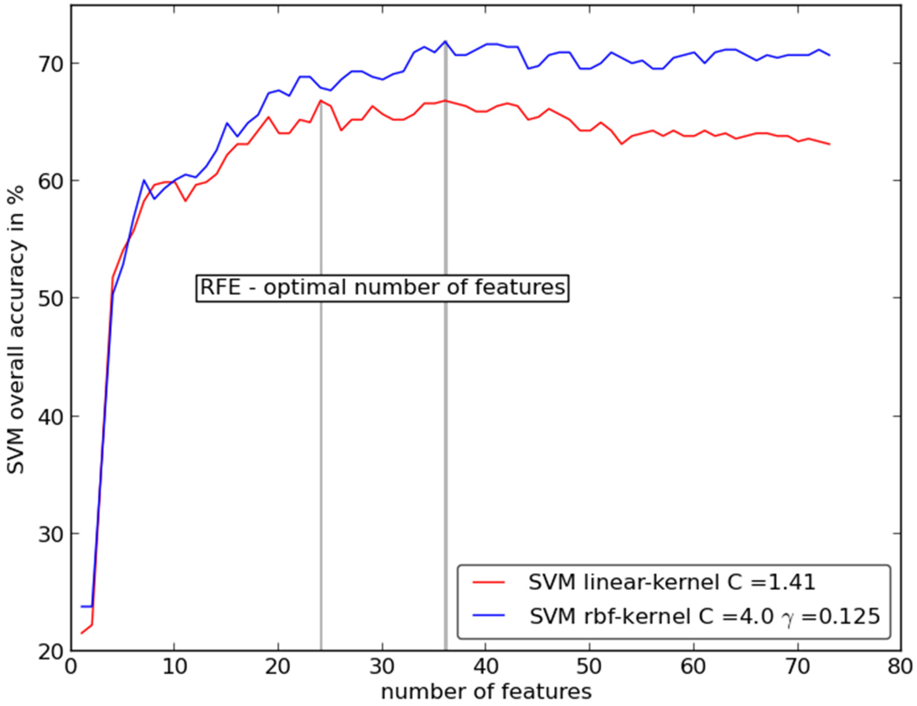
An RFE was performed for the dataset with all 73 input features. The RFE shows that with seven input features, an accuracy exceeding 60% can be attained (Figure 5). The classification accuracy for the SVM, with an RBF-kernel, peaks with a selection of 36 input features, then performs relatively stable until the maximum number of input features is reached. The so-called Hughes phenomenon, which describes the decrease in classification accuracy when additional input features are added to an already large dataset, cannot be observed with the RBF-kernel [100]. Yet, a small decrease can be noted for the linear kernel (Figure 5). The 36 input features from the RFE selection represent all input feature groups (Table 7). Out of the first seven input features, two are topographic indices. The MRRTF results in high values for flat elevated areas [65], and the geomorphons (geomorphologic phonotypes) classify the topography into landscape elements [63]. Both features describe the position of the target classes in the study area. WV2 contributes, along with the spectral Bands 3 and 1, two further input datasets. The ASTER Calcite Index and the Ferric Iron (Fe³+) Index may explain the distribution of the two target classes with high CaCO3 content (Classes 2 and 3) and the topsoil class with iron oxide properties (Class 8). The AlOH Group Index may support the discrimination of clay minerals [56].
Figure 5. Accuracy curves from RFE for a linear and an RBF-kernel.
Remotesensing 07 09563 g005
The confusion matrix of the RFE-selected input feature dataset reveals that the most competitive classes, concerning the user’s and the producer's accuracy, are Class 2 “carbonate-rich substrates” and Class 3 “calcaric topsoil” (Table 8). Both classes have high carbonate content, and the topographic position is overlapping. The difference between both classes is related to the amount of CaCO3 concretions, which are much higher in the lacustrine deposits. If we were to merge both classes, the overall accuracy would reach 79%. However, the visual validation shows a reasonable distribution for both classes. Class 3 also overlaps with Class 4 “dark topsoil”. Class 4 is associated mainly with colluvial and fluvial deposits and shows low CaCO3 content. The transition to Class 3 is gradual. The low producer’s accuracy of Class 5 “tuff outcrop” can be explained by the relatively small area of these outcrops. The producer’s accuracy of this particular class is higher (75%) when only applying the WV2-related input parameters, but the medium-resolution information of the ASTER- and DEM-derived features seems to corrupt the correct identification.
Table 8. Confusion matrix for RFE classification with RBF-kernel (C = 4, g = 0.125).
Classified DataProducers Accuracy
12345 678910
Reference Class16000000000100%
2085000000062%
30512300000060%
40021900000186%
5010051210050%
6000009300075%
70110001200086%
80012001102063%
9002200006060%
100020000001083%
Users Accuracy100%53%48%73%100%90%67%91%75%91%Overall Accuracy 97/135 = 71.9%
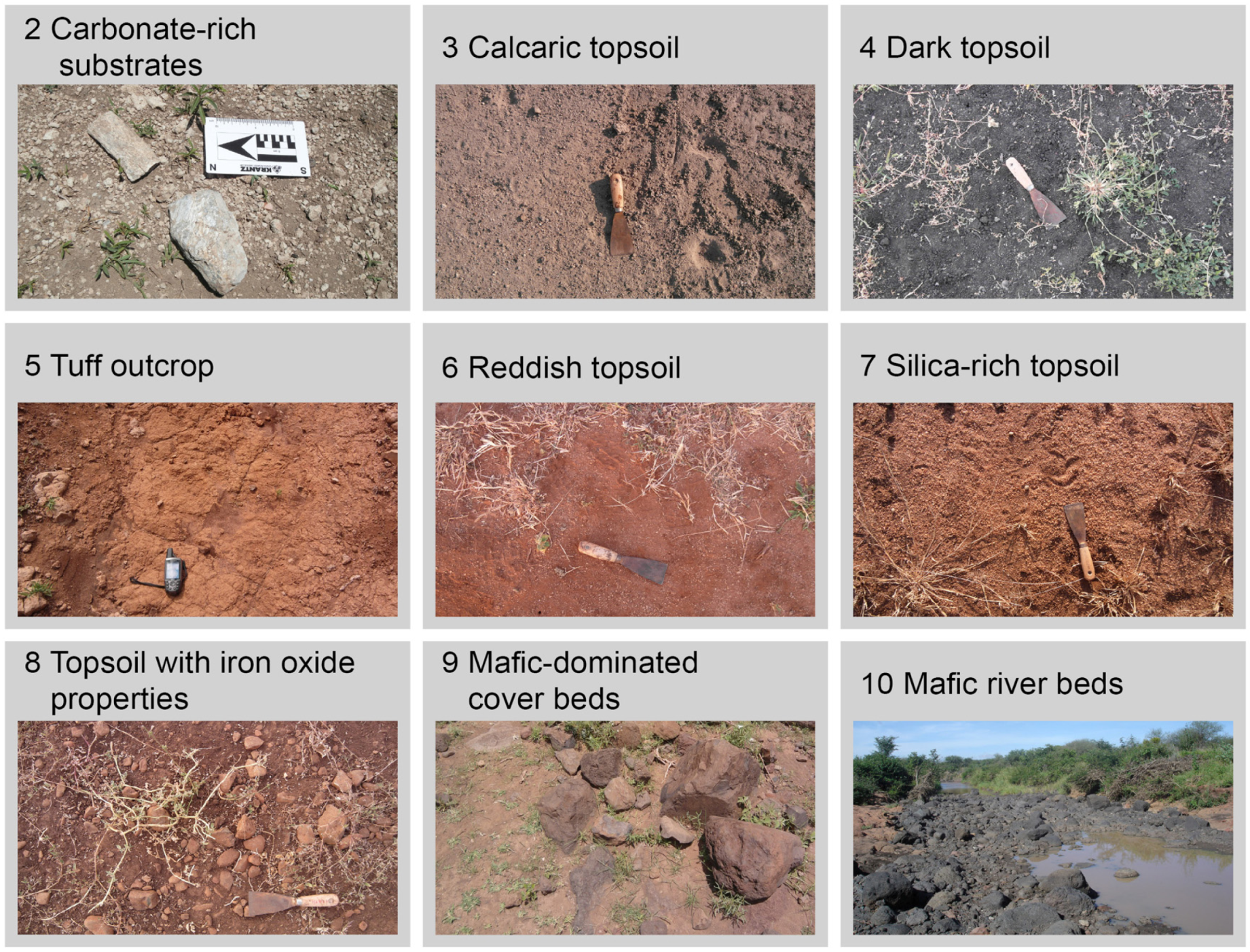
“Carbonate-rich substrates” mainly represent the lacustrine lower member of the Manyara Beds, which are exposed prevalently at the foot of slope and mid-slope positions of the Makuyuni River system, as well as in associated gully systems (Figure 6). The class “calcaric topsoil” indicates soils that show an enrichment of CaCO3 due to inputs from carbonatic volcanic ash deposits or development processes upon the “carbonate-rich substrates”. In some cases, CaCO3-rich soils developed on secondary translocated carbonates or consist of eroded soils exposing CaCO3 concretions. The latter ones were identified during fieldwork in areas with higher slope degrees or large specific catchment areas. “Tuff outcrops” (Class 5) were recognized at a stratigraphic position above the lower member of the Manyara Beds, which coincides with the results of fieldwork and reviewed scientific literature [47]. The outcrops are too minuscule to be displayed in the map (Figure 6). The class “reddish topsoil” is identified with satisfying accuracy. This class is located mainly on stable flat ridge tops and is used agriculturally. Consequently, topsoils are disturbed and reworked by ploughing activity, bringing leached CaCO3 back to the surface (Table 5). This makes the difference in Class 7 “silica-rich topsoil”. These soils are not disturbed, and consequently, silica enriches at the surface due to selective erosion processes. “Silica-rich topsoils” and “reddish topsoils” developed on the Proterozoic intermediate quartzite and gneisses of the Masai Plateau, occur especially in the south of the study area. However, also, these areas were subject to carbonatic volcanic ash deposits. The topsoils with iron oxide properties (Class 8) occur in association with mafic ridges (phonolite, nephelinite) or along the slopes of the Essimingor volcano (Figure 6). Class 9 “Mafic-dominated cover beds” was identified well. Like Class 8, Class 9 can be found at the volcano slopes and on the mafic ridges. Since the cover beds are densely vegetated by shrubs, only small, vegetation-sparse areas were used for the classification. The “mafic river beds” are often covered by vegetation and water. Nevertheless, the mafic material at point bars in the Makuyuni River was traced with high accuracies.
Figure 6. Final classification of topsoil distribution in the study area.
Remotesensing 07 09563 g006
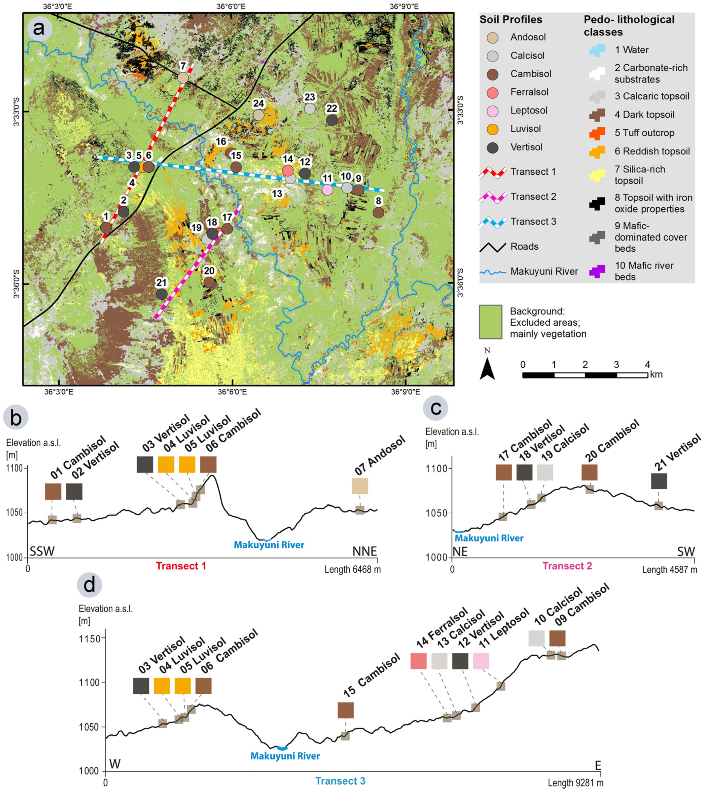
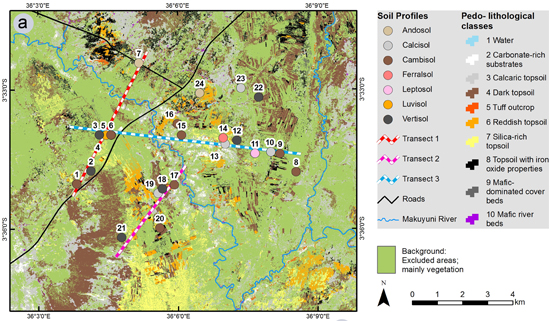
Out of 24 soil profile analyses conducted in the study area, we identified seven main soil types (see Figure 7). In the following, we show that these topsoils can be related to or associated with specific WRB soil types according to the applied catena approach. Vertisols are found in flat areas and in depressions characterized by high clay contents and representing formerly wet positions, related to a high biomass production. They are associated with “dark topsoil” (Class 4). Vertisols occur in association with Vertic Cambisols (Clayic) (Soil Profile 1; Figure 7b) that also relates to the pedo-lithological Class 4 “dark topsoil”. In the study area, Calcisols occur with lacustrine “carbonate-rich substrates” (Class 2) and “calcaric topsoils” (Class 3), which are characterized by eroded Luvisols exposing CaCO3 concretions.
Andosols are located on flat and stable ridge positions with low erosion potential. These soils developed from parent material of volcanic origin, such as volcanic ash, tuff and pumice. They show high mineral proportions indicating fertile soils suitable for crop production. In our analysis, Andosols co-exist with “reddish topsoils” (Class 6). Cambisols are widely distributed in the study area and occur mainly on relatively flat mid-slope positions. Along the Makuyuni River terraces, they are distinguished as Cambisols (Colluvic) (Soil Profiles 15–17; Figure 7). On flat ridge positions, they develop as Andic Cambisol (Soil Profiles 6, 8 and 9, Figure 7). Rhodic Cambisols (Soil Profile 20; Figure 7c) are particularly located on intensively-used agricultural fields and correlate with “reddish topsoils” (Class 6), showing a dark reddish brown 5 YR 3/4 Munsell® color for the first 15 cm of soil depth. Cambisols and Luvisols are associated with each other and correlate with “silica-rich topsoils” (Class 7) and “reddish topsoils” (Class 6). The Haplic Ferralsol (Soil Profile 14; Figure 7d) correlates with “silica-rich topsoil” (Class 7). These soils developed on a weathered felsic basement.
Figure 7. Section of the classification with soil profile transects. (a) Map with soil profile transects; (b) Soil profile transect 1 (SSW – NNE orientation); (c) Soil profile transect 2 (NE–SW orientation); (d) Soil profile transect 3 (W–E orientation).
Remotesensing 07 09563 g007
The resulting map provides a very detailed distribution of topsoils and surface substrates for the study area, which outcompetes other spatial soil information available for this region, like the official soil map by De Pauw [43], the 250 m Africa Soil Information Service (AfSIS) product [42] or the products from the Soil and Terrain Database (SOTER) program [101]. Furthermore, the comparison with the soil profile catenae shows that the detailed topsoil information can be related to specific WRB-based soil types with little additional fieldwork and/or expert knowledge. Nevertheless, providing detailed information on topsoils and surface substrates in comparison to other DSM studies [31,32,42] remains the main intention of the paper.

6. Conclusions

The introduced study has mapped the distribution of topsoils and lithology in a study area in the semiarid Lake Manyara Basin. Applying an integrated approach, combining surface characteristics and terrain features, the spatial distribution of topsoils and related soil types was derived. The topsoils have complex genetic origins related to different substrates, resulting in a high spatial heterogeneity. The non-vegetated areas were classified with a multisensoral approach, which included WV2 and ASTER multispectral data, the TSX1 and Envisat ASAR SAR scenes, and topographical indices were derived from SRTM-X data. With a C-SVC and an RBF-kernel, an overall accuracy of 71.9% was achieved for a challenging classification depth of 10 target classes. The final map is coherent with field observations and laboratory analysis of 27 soil samples. The applied methodological approach seems suitable for multiscale and multisensoral datasets of large areas. We show that the topsoil classification can be associated with soil profiles obtained by fieldwork and certain terrain positions derived from DEM, thus allowing a distinct spatial attribution of soil types.
The results of the topsoil classification and the related soil type association give valuable information, which can help to find locations for agricultural projects in the region and may thereby support the transition to the sustainable self-subsistence of the local population. This may contribute to a reduction of cattle-induced overgrazing and subsequent land degradation. For many applications, like archaeological field studies and paleontological surveys, high-resolution topsoil and surface substrate information yields greater insight than low-resolution soil type maps. The results of this work also help to explain the geological situation of the study area and the landscape evolution. Despite the potential influence of different fluvial and mass movement processes on the topsoil distribution, this study draws a valuable picture of the general situation.

Acknowledgments

This study was financed by the Heidelberg Academy of Sciences and Humanities research center: “The Role of Culture in Early Expansions of Humans” (ROCEEH). The WorldView-2 scene is courtesy of the DigitalGlobe Foundation. We would like to thank the DLR and the German Remote Sensing Data Center (DFD) for providing the TerraSAR-X and the SRTM/X-SAR data. The European Space Agency (ESA) provided the Envisat ASAR data. We acknowledge the support of Deutsche Forschungsgemeinschaft and Open Access Publishing Fund of Tuebingen University. We also want to acknowledge the EU International Research Staff Exchange Scheme (IRSES) Fluvial processes and sediment dynamics of slope channel systems (FLUMEN) (PIRSES-GA-2012-318969) project financing the exchange of researchers.

Author Contributions

Felix Bachofer designed and implemented the research of this study. He processed the remote sensing data, conducted the analysis and drafted the manuscript. Geraldine Quénéhervé analyzed the soil profiles. Felix Bachofer, Geraldine Quénéhervé and Michael Maerker contributed to the collection of ground reference data during three field campaigns from 2010–2014. Furthermore, Felix Bachofer, Geraldine Quénéhervé, Volker Hochschild and Michael Maerker contributed to the data interpretation and supervised the manuscript construction.

Conflicts of Interest

The authors declare no conflict of interest.

References

  1. Solomon, A.M.; Webb, T., III. Computer-aided reconstruction of late-quaternary landscape dynamics. Annu. Rev. Ecol. Syst. 1985, 16, 63–84. [Google Scholar] [CrossRef]
  2. Moore, I.D.; Gessler, P.E.; Nielsen, G.A.; Peterson, G.A. Soil attribute prediction using terrain analysis. Soil Sci. Soc. Am. J. 1993, 57, 443–452. [Google Scholar] [CrossRef]
  3. Sabins, F.F. Remote sensing for mineral exploration. Ore Geol. Rev. 1999, 14, 157–183. [Google Scholar] [CrossRef]
  4. Anderson, K.; Croft, H. Remote sensing of soil surface properties. Prog. Phys. Geogr. 2009, 33, 457–473. [Google Scholar] [CrossRef]
  5. Mulder, V.L.; de Bruin, S.; Schaepman, M.E.; Mayr, T.R. The use of remote sensing in soil and terrain mapping—A review. Geoderma 2011, 162, 1–19. [Google Scholar] [CrossRef]
  6. Dewitte, O.; Jones, A.; Elbelrhiti, H.; Horion, S.; Montanarella, L. Satellite remote sensing for soil mapping in Africa: An overview. Prog. Phys. Geogr. 2012, 36, 514–538. [Google Scholar] [CrossRef]
  7. FAO. Topsoil Characterization for Sustainable Land Management, Draft; Food and Agriculture Organization of the United Nations, Land and Water Development Division, Soil Resources, Management and Conservation Service: Rome, Italy, 1998; p. 74. Available online: ftp://ftp.fao.org/agl/agll/docs/topsoil.pdf (accessed on 23 July 2015).
  8. USDA (United States Department of Agriculture). Soil Survey Manual; Soil Survey Division: Washington, DC, USA, 1993; p. 437.
  9. Broll, G.; Brauckmann, H.J.; Overesch, M.; Junge, B.; Erber, C.; Milbert, G.; Baize, D.; Nachtergaele, F. Topsoil characterization-recommendations for revision and expansion of the FAO-Draft (1998) with emphasis on humus forms and biological features. J. Plant Nutr. Soil Sci. 2006, 169, 453–461. [Google Scholar] [CrossRef]
  10. Graefe, U.; Baritz, R.; Broll, G.; Kolb, E.; Milbert, G.; Wachendorf, C. Adapting humus form classification to WRB principles. In Proceedings of the 4th International Congress of the European Soil Science Societies—Eurosoil, Bari, Italy, 2–6 July 2012; p. 954.
  11. Ben-Dor, E.; Goldlshleger, N.; Benyamini, Y.; Agassi, M.; Blumberg, D.G. The spectral reflectance properties of soil structural crusts in the 1.2- to 2.5-μm spectral region. Soil Sci. Soc. Am. J. 2003, 67, 289–299. [Google Scholar] [CrossRef]
  12. Baghdadi, N.; Cerdan, O.; Zribi, M.; Auzet, V.; Darboux, F.; El Hajj, M.; Kheir, R.B. Operational performance of current synthetic aperture radar sensors in mapping soil surface characteristics in agricultural environments: Application to hydrological and erosion modelling. Hydrol. Process. 2008, 22, 9–20. [Google Scholar] [CrossRef]
  13. Aubert, M.; Baghdadi, N.; Zribi, M.; Douaoui, A.; Loumagne, C.; Baup, F.; El Hajj, M.; Garrigues, S. Analysis of TerraSAR-X data sensitivity to bare soil moisture, roughness, composition and soil crust. Remote Sens. Environ. 2011, 115, 1801–1810. [Google Scholar] [CrossRef] [Green Version]
  14. Aubert, M.; Baghdadi, N.N.; Zribi, M.; Ose, K.; El Hajj, M.; Vaudour, E.; Gonzalez-Sosa, E. Toward an operational bare soil moisture mapping using TerraSAR-X data acquired over agricultural areas. IEEE J. Sel. Top. Appl. Earth Obs. Remote Sens. 2013, 6, 900–916. [Google Scholar] [CrossRef] [Green Version]
  15. Schmugge, T.J.; Kustas, W.P.; Ritchie, J.C.; Jackson, T.J.; Rango, A. Remote sensing in hydrology. Adv. Water Resour. 2002, 25, 1367–1385. [Google Scholar] [CrossRef]
  16. Ben-Dor, E.; Chabrillat, S.; Demattê, J.A.M.; Taylor, G.R.; Hill, J.; Whiting, M.L.; Sommer, S. Using imaging spectroscopy to study soil properties. Remote Sens. Environ. 2009, 113 (Suppl. 1), S38–S55. [Google Scholar] [CrossRef]
  17. Bartholomeus, H.; Epema, G.; Schaepman, M. Determining iron content in Mediterranean soils in partly vegetated areas, using spectral reflectance and imaging spectroscopy. Int. J. Appl. Earth Obs. Geoinf. 2007, 9, 194–203. [Google Scholar] [CrossRef] [Green Version]
  18. Grebby, S.; Cunningham, D.; Tansey, K.; Naden, J. The impact of vegetation on lithological mapping using airborne multispectral data: A case study for the north Troodos region, Cyprus. Remote Sens. 2014, 6, 10860–10887. [Google Scholar] [CrossRef]
  19. Rouse, J.W.; Haas, R.H.; Shell, J.A.; Deering, D.W.; Harlan, J.C. Monitoring the Vernal Advancement of Retrogradation of Natural Vegetation; NASA/GSFC: Greenbelt, MD, USA, 1974; p. 371.
  20. Yang, X.; Guo, X. Quantifying responses of spectral vegetation indices to dead materials in mixed grasslands. Remote Sens. 2014, 6, 4289–4304. [Google Scholar] [CrossRef]
  21. Pickup, G.; Chewings, V.H.; Nelson, D.J. Estimating changes in vegetation cover over time in arid rangelands using landsat MSS data. Remote Sens. Environ. 1993, 43, 243–263. [Google Scholar] [CrossRef]
  22. Trodd, N.M.; Dougill, A.J. Monitoring vegetation dynamics in semi-arid African rangelands: Use and limitations of earth observation data to characterize vegetation structure. Appl. Geogr. 1998, 18, 315–330. [Google Scholar] [CrossRef]
  23. Mitchell, J.; Shrestha, R.; Moore-Ellison, C.; Glenn, N. Single and multi-date Landsat classifications of basalt to support soil survey efforts. Remote Sens. 2013, 5, 4857–4876. [Google Scholar] [CrossRef]
  24. Dogan, H.M.; Kılıç, O.M. Modelling and mapping some soil surface properties of Central Kelkit Basin in Turkey by using Landsat-7 ETM+ images. Int. J. Remote Sens. 2013, 34, 5623–5640. [Google Scholar] [CrossRef]
  25. Rowan, L.C.; Mars, J.C. Lithologic mapping in the Mountain Pass, California area using Advanced Spaceborne Thermal Emission and Reflection Radiometer (ASTER) data. Remote Sens. Environ. 2003, 84, 350–366. [Google Scholar] [CrossRef]
  26. Rowan, L.C.; Mars, J.C.; Simpson, C.J. Lithologic mapping of the Mordor, NT, Australia ultramafic complex by using the Advanced Spaceborne Thermal Emission and Reflection Radiometer (ASTER). Remote Sens. Environ. 2005, 99, 105–126. [Google Scholar] [CrossRef]
  27. Mars, J.C.; Rowan, L.C. Spectral assessment of new ASTER SWIR surface reflectance data products for spectroscopic mapping of rocks and minerals. Remote Sens. Environ. 2010, 114, 2011–2025. [Google Scholar] [CrossRef]
  28. Pour, A.B.; Hashim, M. Application of advanced spaceborne thermal emission and reflection radiometer (ASTER) data in geological mapping. Int. J. Phys. Sci. 2011, 6, 7657–7668. [Google Scholar]
  29. Vicente, L.E.; de Souza Filho, C.R. Identification of mineral components in tropical soils using reflectance spectroscopy and advanced spaceborne thermal emission and reflection radiometer (ASTER) data. Remote Sens. Environ. 2011, 115, 1824–1836. [Google Scholar] [CrossRef]
  30. Conacher, A.J.; Dalrymple, J.B. The nine unit land surface model and pedogeomorphic research. Geoderma 1977, 18, 127–144. [Google Scholar]
  31. Mulder, V.L.; de Bruin, S.; Weyermann, J.; Kokaly, R.F.; Schaepman, M.E. Characterizing regional soil mineral composition using spectroscopy and geostatistics. Remote Sens. Environ. 2013, 139, 415–429. [Google Scholar] [CrossRef]
  32. Hahn, C.; Gloaguen, R. Estimation of soil types by non linear analysis of remote sensing data. Nonlinear Process. Geophys. 2008, 15, 115–126. [Google Scholar] [CrossRef]
  33. Rossel, R.A.V.; Chen, C. Digitally mapping the information content of visible–near infrared spectra of surficial Australian soils. Remote Sens. Environ. 2011, 115, 1443–1455. [Google Scholar] [CrossRef]
  34. Selige, T.; Böhner, J.; Schmidhalter, U. High resolution topsoil mapping using hyperspectral image and field data in multivariate regression modeling procedures. Geoderma 2006, 136, 235–244. [Google Scholar] [CrossRef]
  35. Gaber, A.; Koch, M.; El-Baz, F. Textural and compositional characterization of Wadi Feiran deposits, Sinai Peninsula, Egypt, using Radarsat-1, PALSAR, SRTM and ETM+ Data. Remote Sens. 2010, 2, 52–75. [Google Scholar] [CrossRef]
  36. Zribi, M.; Chahbi, A.; Shabou, M.; Lili-Chabaane, Z.; Duchemin, B.; Baghdadi, N.; Amri, R.; Chehbouni, A. Soil surface moisture estimation over a semi-arid region using ENVISAT ASAR radar data for soil evaporation evaluation. Hydrol. Earth Syst.Sci. 2011, 15, 345–358. [Google Scholar] [CrossRef] [Green Version]
  37. Zribi, M.; Kotti, F.; Lili-Chabaane, Z.; Baghdadi, N.; Ben Issa, N.; Amri, R.; Duchemin, B.; Chehbouni, A. Soil texture estimation over a semiarid area using TerraSAR-X radar data. IEEE Geosci. Remote Sens. Lett. 2012, 9, 353–357. [Google Scholar] [CrossRef] [Green Version]
  38. Baghdadi, N.; Aubert, M.; Zribi, M. Use of TerraSAR-X data to retrieve soil moisture over bare soil agricultural fields. IEEE Geosci. Remote Sens. Lett. 2012, 9, 512–516. [Google Scholar] [CrossRef] [Green Version]
  39. Vaudour, E.; Baghdadi, N.; Gilliot, J.M. Mapping tillage operations over a peri-urban region using combined SPOT4 and ASAR/ENVISAT images. Int. J. Appl. Earth Obs. Geoinf. 2014, 28, 43–59. [Google Scholar] [CrossRef]
  40. Gorrab, A.; Zribi, M.; Baghdadi, N.; Mougenot, B.; Chabaane, Z. Potential of X-band TerraSAR-X and COSMO-SkyMed SAR data for the assessment of physical soil parameters. Remote Sens. 2015, 7, 747–766. [Google Scholar] [CrossRef] [Green Version]
  41. Baghdadi, N.; Cresson, R.; El Hajj, M.; Ludwig, R.; la Jeunesse, I. Estimation of soil parameters over bare agriculture areas from C-band polarimetric SAR data using neural networks. Hydrol. Earth Syst. Sci. 2012, 16, 1607–1621. [Google Scholar] [CrossRef] [Green Version]
  42. Hengl, T.; Heuvelink, G.B.M.; Kempen, B.; Leenaars, J.G.B.; Walsh, M.G.; Shepherd, K.D.; Sila, A.; MacMillan, R.A.; Mendes de Jesus, J.; Tamene, L.; et al. Mapping soil properties of Africa at 250 m resolution: Random forests significantly improve current predictions. PLoS One 2015, 10, e0125814. [Google Scholar] [CrossRef] [PubMed]
  43. De Pauw, E. Soils, physiography and agro-ecological zones of tanzania. In Crop Monitoring and Early Warning Systems Project, Food and Agriculture Organization of the United Nations. GCPS/URT/047/NET; Ministry of Agriculture: Dar es Salaam, Tanzania, 1983. [Google Scholar]
  44. Huffman, G.J.; Adler, R.F.; Bolvin, D.T.; Gu, G.J.; Nelkin, E.J.; Bowman, K.P.; Hong, Y.; Stocker, E.F.; Wolff, D.B. The TRMM multisatellite precipitation analysis (TMPA): Quasi-global, multiyear, combined-sensor precipitation estimates at fine scales. J. Hydrometeorol. 2007, 8, 38–55. [Google Scholar] [CrossRef]
  45. Bachofer, F.; Quénéhervé, G.; Märker, M. The delineation of paleo-shorelines in the Lake Manyara basin using TerraSAR-X data. Remote Sens. 2014, 6, 2195–2212. [Google Scholar] [CrossRef]
  46. Kiunsi, R.B.; Meadows, M.E. Assessing land degradation in the Monduli District, northern Tanzania. Land Degrad. Dev. 2006, 17, 509–525. [Google Scholar] [CrossRef]
  47. Schwartz, H.; Renne, P.R.; Morgan, L.E.; Wildgoose, M.M.; Lippert, P.C.; Frost, S.R.; Harvati, K.; Schrenk, F.; Saanane, C. Geochronology of the Manyara Beds, northern Tanzania: New tephrostratigraphy, magnetostratigraphy and 40Ar/39Ar ages. Quat. Geochronol. 2012, 7, 48–66. [Google Scholar] [CrossRef]
  48. Dawson, J.B. The Gregory Rift Valley and Neogene-Recent Volcanoes of Northern Tanzania; Geological Society: London, UK, 2008; p. 102. [Google Scholar]
  49. Dawson, J.B. Neogene tectonics and volcanicity in the North Tanzania sector of the Gregory Rift Valley: Contrasts with the Kenya sector. Tectonophysics 1992, 204, 81–92. [Google Scholar] [CrossRef]
  50. Ring, U.; Schwartz, H.L.; Bromage, T.G.; Sanaane, C. Kinematic and sedimentological evolution of the Manyara Rift in northern Tanzania, East Africa. Geol. Mag. 2005, 142, 355–368. [Google Scholar] [CrossRef]
  51. Frost, S.R.; Schwartz, H.L.; Giemsch, L.; Morgan, L.E.; Renne, P.R.; Wildgoose, M.; Saanane, C.; Schrenk, F.; Harvati, K. Refined age estimates and Paleoanthropological investigation of the Manyara Beds, Tanzania. J. Anthropol. Sci. 2012, 90, 151–161. [Google Scholar] [PubMed]
  52. Bachofer, F.; Quénéhervé, G.; Märker, M.; Hochschild, V. Comparison of SVM and boosted regression trees for the delineation of lacustrine sediments using multispectral ASTER data and topographic indices in the Lake Manyara basin. Photogramm. Fernerkund. Geoinf. 2015, 1, 81–94. [Google Scholar] [CrossRef]
  53. DigitalGlobe WorldView-2. Available online: https://www.digitalglobe.com/sites/default/files/DG_WorldView2_DS_PROD.pdf (accessed on 20 January 2015).
  54. Yamaguchi, Y.; Kahle, A.B.; Tsu, H.; Kawakami, T.; Pniel, M. Overview of advanced spaceborne thermal emission and reflection radiometer (ASTER). IEEE Trans. Geosci. Remote Sens. 1998, 36, 1062–1071. [Google Scholar] [CrossRef]
  55. Iwasaki, A.; Fujisada, H.; Akao, H.; Shindou, O.; Akagi, S. Enhancement of spectral separation performance for ASTER/SWIR. Proc. SPIE 2002, 4486, 42–50. [Google Scholar]
  56. Cudahy, T. Satellite ASTER Geoscience Product—Notes for Australia; Commonwealth Scientific and Industrial Research Organisation (CSIRO): Dickson, Australia, 2012; p. 26. [Google Scholar]
  57. Bierwirth, P. Evaluation of ASTER Satellite Data for Geological Applications; Consultancy Report to Geoscience Australia: Canberra, Australia, 2002; p. 50. [Google Scholar]
  58. Hewson, R.D.; Cudahy, T.J.; Mizuhiko, S.; Ueda, K.; Mauger, A.J. Seamless geological map generation using ASTER in the Broken Hill-Curnamona province of Australia. Remote Sens. Environ. 2005, 99, 159–172. [Google Scholar] [CrossRef]
  59. Ninomiya, Y.; Fu, B.; Cudahy, T.J. Detecting lithology with Advanced Spaceborne Thermal Emission and Reflection Radiometer (ASTER) multispectral thermal infrared “radiance-at-sensor” data. Remote Sens. Environ. 2005, 99, 127–139. [Google Scholar] [CrossRef]
  60. Hoffmann, J.; Walter, D. How complementary are SRTM-X and -C band digital elevation models? Photogramm. Eng. Remote Sens. 2006, 72/3, 261–268. [Google Scholar] [CrossRef]
  61. Lee, J.S. Digital image enhancement and noise filtering by use of local statistics. IEEE Trans. Pattern Anal. Mach. Intell. 1980, 2, 165–168. [Google Scholar] [CrossRef] [PubMed]
  62. DLR SRTM Digital Elevation Models/SRTM-X Specifications. Available online: https://centaurus.caf.dlr.de:8443/eoweb-ng/licenseAgreements/DLR_SRTM_Readme.pdf (accessed on 3 April 2015).
  63. Jasiewicz, J.; Stepinski, T.F. Geomorphons—A pattern recognition approach to classification and mapping of landforms. Geomorphology 2013, 182, 147–156. [Google Scholar] [CrossRef]
  64. Moore, I.D.; Grayson, R.B.; Ladson, A.R. Digital terrain modelling: A review of hydrological, geomorphological, and biological applications. Hydrol. Process. 1991, 5, 3–30. [Google Scholar] [CrossRef]
  65. Gallant, J.C.; Dowling, T.I. A multiresolution index of valley bottom flatness for mapping depositional areas. Water Resour. Res. 2003, 39, 1347. [Google Scholar] [CrossRef]
  66. Yokoyama, R.; Shirasawa, M.; Pike, R.J. Visualizing topography by openness: A new application of image processing to digital elevation models. Photogramm. Eng. Remote Sens. 2002, 68, 257–266. [Google Scholar]
  67. Zevenbergen, L.W.; Thorne, C.R. Quantitative analysis of land surface topography. Earth Surf. Proc. Landf. 1987, 12, 47–56. [Google Scholar] [CrossRef]
  68. Dikau, R. Entwurf Einer Geomorphographisch-Analytischen Systematik von Reliefeinheiten; Heidelberger Geographische Bausteine: Heidelberg, Germany, 1988. [Google Scholar]
  69. Travis, M.R.; Elsner, G.H.; Iverson, W.D.; Johnson, C.G. VIEWIT: Computation of Seen Areas, Slope, and Aspect for Land-Use Planning; Pacific Southwest Research Station, Forest Service, U.S. Department of Agriculture: Berkeley, CA, USA, 1975.
  70. Bock, M.; Böhner, J.; Conrad, O.; Köthe, R.; Ringeler, A. Methods for Creating Functional Soil Databases and Applying Digital Soil Mapping with SAGA GIS. In Status and Prospect of Soil Information in South-Eastern Europe; Office for Official Publications of the European Communities: Luxembourg, 2007; pp. 149–162. [Google Scholar]
  71. Riley, S.J.; DeGloria, S.D.; Elliot, R. A terrain ruggedness index that Quantifies topographic heterogeneity. Intermt. J. Sci. 1999, 5, 23–27. [Google Scholar]
  72. Guisan, A.; Weiss, S.; Weiss, A. GLM versus CCA spatial modeling of plant species distribution. Plant Ecol. 1999, 143, 107–122. [Google Scholar] [CrossRef]
  73. Beven, K.; Kirkby, M.J. A physically based, variable contributing area model of basin hydrology. Hydrol. Sci. J. 1979, 24, 43–69. [Google Scholar]
  74. Conrad, O. Terrain Parameters described in the SAGA-GIS Software v.2.1.0. Available online: http://sourceforge.net/projects/saga-gis/files/latest/download?source=files (accessed on 10 February 2015).
  75. Baghdadi, N.; Camus, P.; Beaugendre, N.; Issa, O.M.; Zribi, M.; Desprats, J.F.; Rajot, J.L.; Abdallah, C.; Sannier, C. Estimating surface soil moisture from TerraSAR-X data over two small catchments in the Sahelian part of western Niger. Remote Sens. 2011, 3, 1266–1283. [Google Scholar] [CrossRef] [Green Version]
  76. Buurman, P.; Lagen, B.V.; Velthorst, E.J.; Lagen, B.; Velthorst, E. Manual for Soil and Water Analysis; Backhuys: Leiden, The Netherlands, 1996. [Google Scholar]
  77. Springer, U.; Klee, J. Prüfung der Leistungsfähigkeit von einigen wichtigeren Verfahren zur Bestimmung des Kohlenstoffs mittels Chromschwefelsäure sowie Vorschlag einer neuen Schnellmethode. J. Soil Sci. Plant Nutr. 1954, 64, 1–26. [Google Scholar] [CrossRef]
  78. Lindsay, W.L.; Norvell, W.A. Development of a dtpa soil test for zinc, iron, manganese, and copper. Soil Sci. Soc. Am. J. 1978, 42, 421–428. [Google Scholar] [CrossRef]
  79. Mehlich, A. Mehlich-3 soil test extractant—A modification of mehlich-2 extractant. Commun. Soil Sci. Plant Anal. 1984, 15, 1409–1416. [Google Scholar] [CrossRef]
  80. FAO. World Reference Base for Soil Resources 2014—International Soil Classification System for Naming Soils and Creating Legends for Soil Maps; Food and Agriculture Organization of the United Nations: Rome, Italy, 2014. [Google Scholar]
  81. Baatz, M.; Schäpe, A. Multiresolution Segmentation: An optimization approach for high quality multi-scale image segmentation. In Angewandte Geographische Informationsverarbeitung XII. Beiträge zum AGIT-Symposium Salzburg; Strobl, J., Blaschke, T., Griesebner, G., Eds.; Wichmann: Heidelberg, Germany, 2000; Volume 12, pp. 12–23. [Google Scholar]
  82. Benz, U.C.; Hofmann, P.; Willhauck, G.; Lingenfelder, I.; Heynen, M. Multi-resolution, object-oriented fuzzy analysis of remote sensing data for GIS-ready information. ISPRS J. Photogramm. Remote Sens. 2004, 58, 239–258. [Google Scholar] [CrossRef]
  83. Haralick, R.M.; Shanmugam, K.; Dinstein, I.H. Textural features for image classification. IEEE Trans. Syst. Man Cybern. 1973, SMC-3, 610–621. [Google Scholar] [CrossRef]
  84. Vapnik, V.N. The Nature of Statistical Learning Theory; Springer: New York, NY, USA, 1995; p. 188. [Google Scholar]
  85. Vapnik, V.N. An overview of statistical learning theory. IEEE Trans. Neural Netw. 1999, 10, 988–999. [Google Scholar] [CrossRef] [PubMed]
  86. Hearst, M.A. Support vector machines. IEEE Intell. Syst. 1998, 13, 18–28. [Google Scholar] [CrossRef]
  87. Burges, C. A tutorial on support vector machines for pattern recognition. Data Min. Knowl. Discov. 1998, 2, 121–167. [Google Scholar] [CrossRef]
  88. Schölkopf, B.; Smola, A.J. A short introduction to learning with kernels. In Advanced Lectures on Machine Learning; Mendelson, S., Smola, A.J., Eds.; Springer-Verlag: Berlin/Heidelberg, Germany, 2003; pp. 41–64. [Google Scholar]
  89. Mountrakis, G.; Im, J.; Ogole, C. Support vector machines in remote sensing: A review. ISPRS J. Photogramm. Remote Sens. 2011, 66, 247–259. [Google Scholar] [CrossRef]
  90. Wang, X.; Niu, R.; Wu, K. Lithology intelligent identification using support vector machine and adaptive cellular automata in multispectral remote sensing image. Opt. Eng. 2011, 50, 076201. [Google Scholar] [CrossRef]
  91. Othman, A.; Gloaguen, R. Improving lithological mapping by SVM classification of spectral and morphological features: The discovery of a new chromite body in the Mawat ophiolite complex (Kurdistan, NE Iraq). Remote Sens. 2014, 6, 6867–6896. [Google Scholar] [CrossRef]
  92. Cortes, C.; Vapnik, V. Support-vector networks. Mach. Learn. 1995, 20, 273–297. [Google Scholar] [CrossRef]
  93. Schölkopf, B.; Smola, A.J. Learning with Kernels: Support Vector Machines, Regularization, Optimization, and Beyond; MIT Press: Cambridge, MA, USA, 2002; p. 626. [Google Scholar]
  94. Chang, C.C.; Lin, C.J. LIBSVM: A library for support vector machines. ACM Trans. Intell. Syst. Technol. 2011, 2, 1–27. [Google Scholar] [CrossRef]
  95. Foody, G.M.; Mathur, A. Toward intelligent training of supervised image classifications: Directing training data acquisition for SVM classification. Remote Sens. Environ. 2004, 93, 107–117. [Google Scholar] [CrossRef]
  96. Guyon, I.; Elisseeff, A. An introduction to variable and feature selection. J. Mach. Learn. Res. 2003, 3, 1157–1182. [Google Scholar]
  97. Kohavi, R.; John, G.H. Wrappers for feature subset selection. Artif. Intell. 1997, 97, 273–324. [Google Scholar] [CrossRef]
  98. Guyon, I.; Weston, J.; Barnhill, S.; Vapnik, V. Gene selection for cancer classification using support vector machines. Mach. Learn. 2002, 46, 389–422. [Google Scholar] [CrossRef]
  99. Karatzoglou, A.; Meyer, D.; Hornik, K. Support vector machines in R. J. Stat. Softw. 2006, 15, 1–28. [Google Scholar]
  100. Pal, M.; Foody, G.M. Feature selection for classification of hyperspectral data by SVM. IEEE Trans. Geosci. Remote Sens. 2010, 48, 2297–2307. [Google Scholar] [CrossRef]
  101. ISRIC. Global and National Soils and Terrain Databases (SOTER). In Procedures Manual, Version 2.0; ISRIC—World Soil Information: Wageningen, The Netherlands, 2013; p. 198. [Google Scholar]

