
Sensitivity of Multi-Source SAR Backscatter to Changes in Forest Aboveground Biomass


Abstract
:
1. Introduction
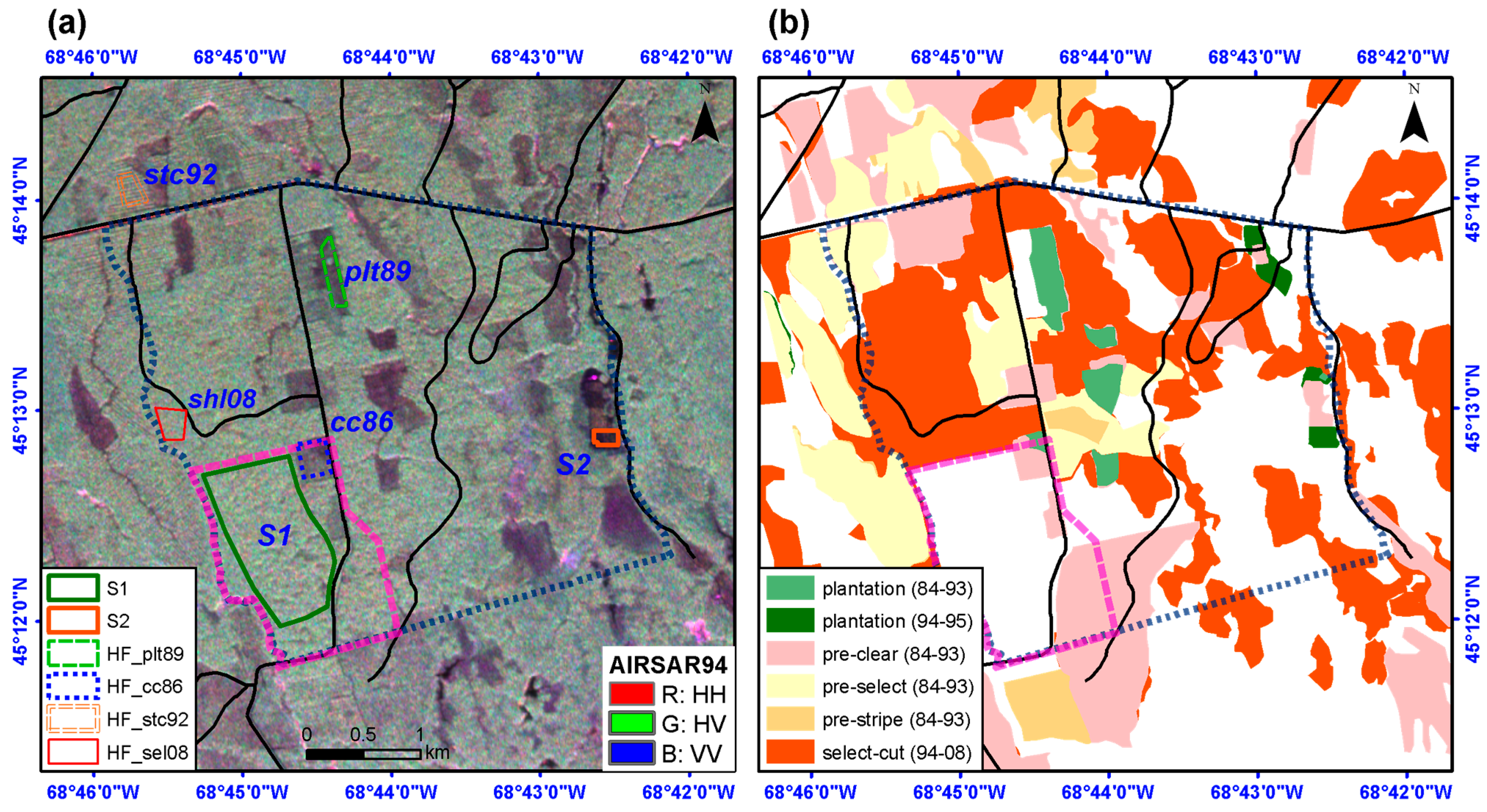
2. Study Area and Data
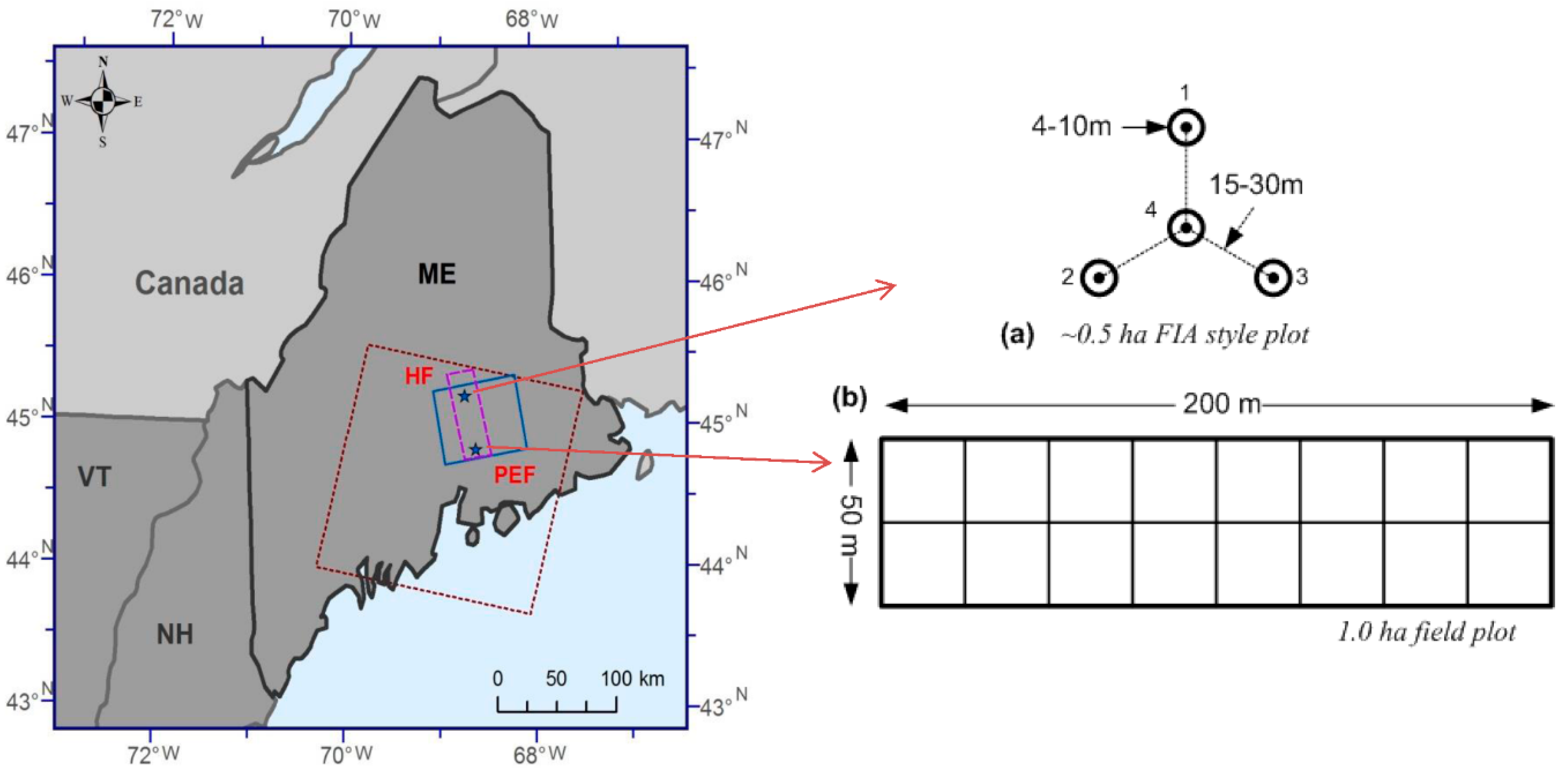
2.1. Field Campaign
2.2. SAR Data

| Sensor | Scene ID | Acquisition Date | Pixel Size* (m) | Incidence Angle# (°) | Environmental Conditions | |||
|---|---|---|---|---|---|---|---|---|
| Temperature (°C) | Precipitation (mm) | |||||||
| 3 Day | 7 Day | 14 Day | ||||||
| SIR-C/XSAR | PR12331 | 04/13/1994 | 12.5 | 31.7 | T ~ 5.5 °C | 17.3 | 42.1 | 50.9 |
| SIR-C/XSAR | PR47494 | 10/04/1994 | 12.5 | 31.7 | T ~ 10.1 °C | 0 | 0.2 | 76 |
| AIRSAR | / | 09/02/1989 | 10 | 35.0 | T ~ 10.1 °C | 16.8 | 18.6 | 27.6 |
| AIRSAR | CM6221 | 10/07/1994 | 10 | 35.0 | T ~ 10.1 °C | 0 | 0.2 | 76 |
| UAVSAR | 16702_09054_016 | 08/05/2009 | 6 | 48.0 | T ~ 21.6 °C | 11.5 | 49.6 | 94.4 |
| PALSAR/FBD | ALPSRP191680890 | 08/30/2009 | 20 | 34.3 | T ~ 14.8 °C | 20.4 | 32 | 34.2 |
2.3. Auxiliary Data
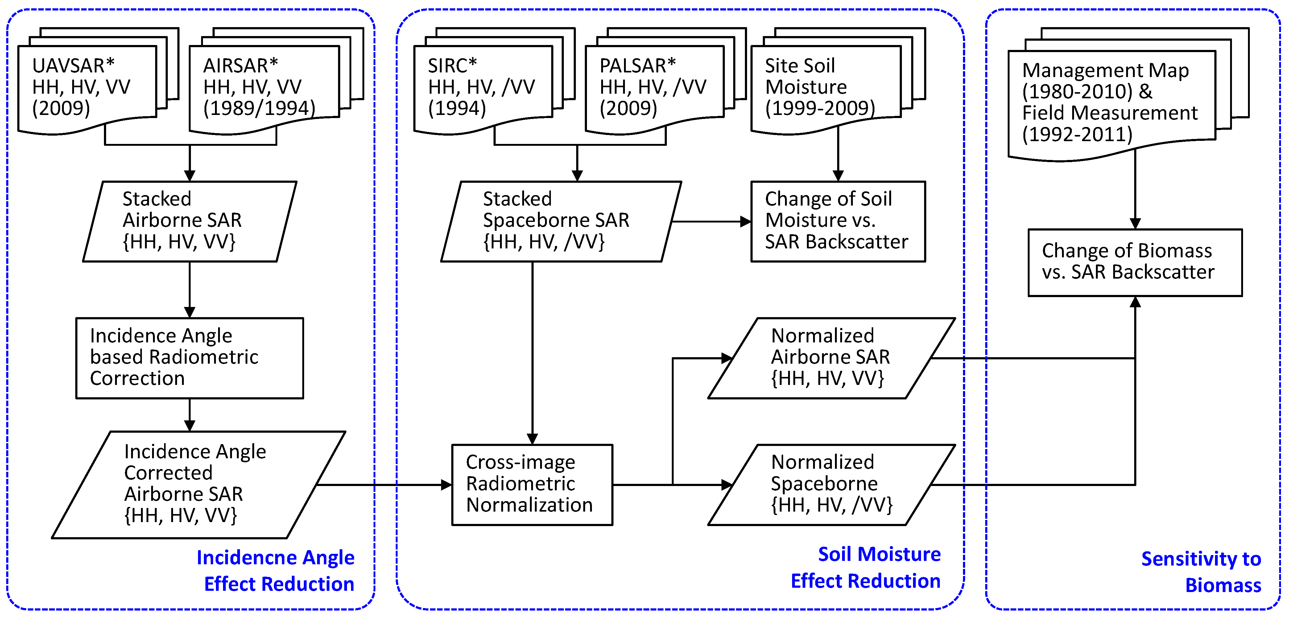
3. Methodology

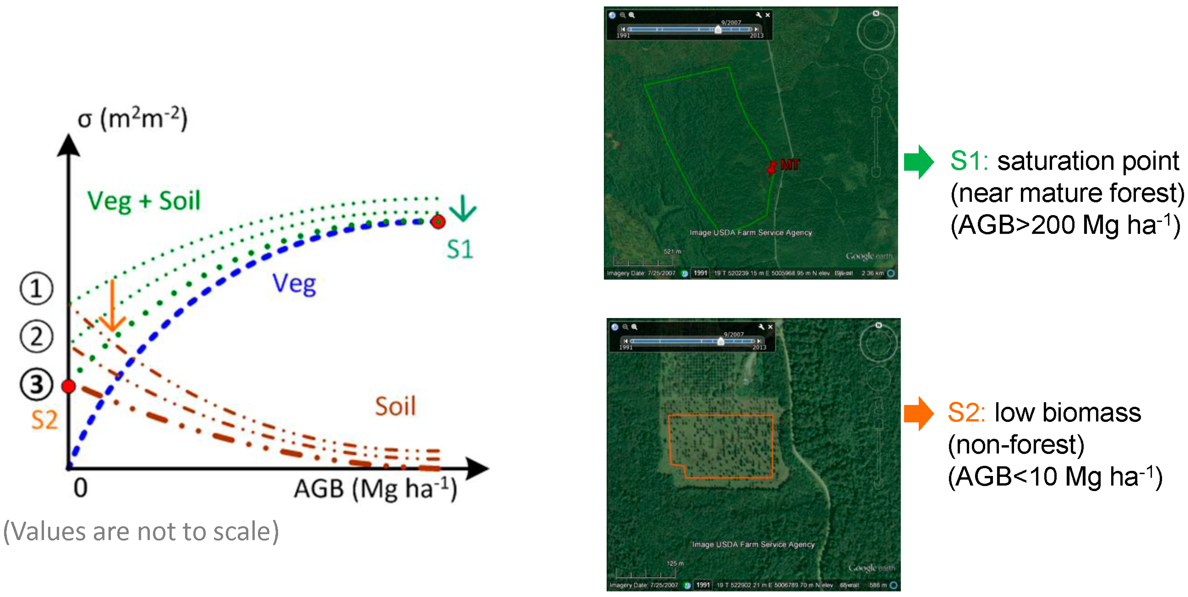
3.1. Sensitivity of SAR Backscatter to Biomass

3.2. Incidence-Angle-Based Correction for Airborne SAR Backscatter
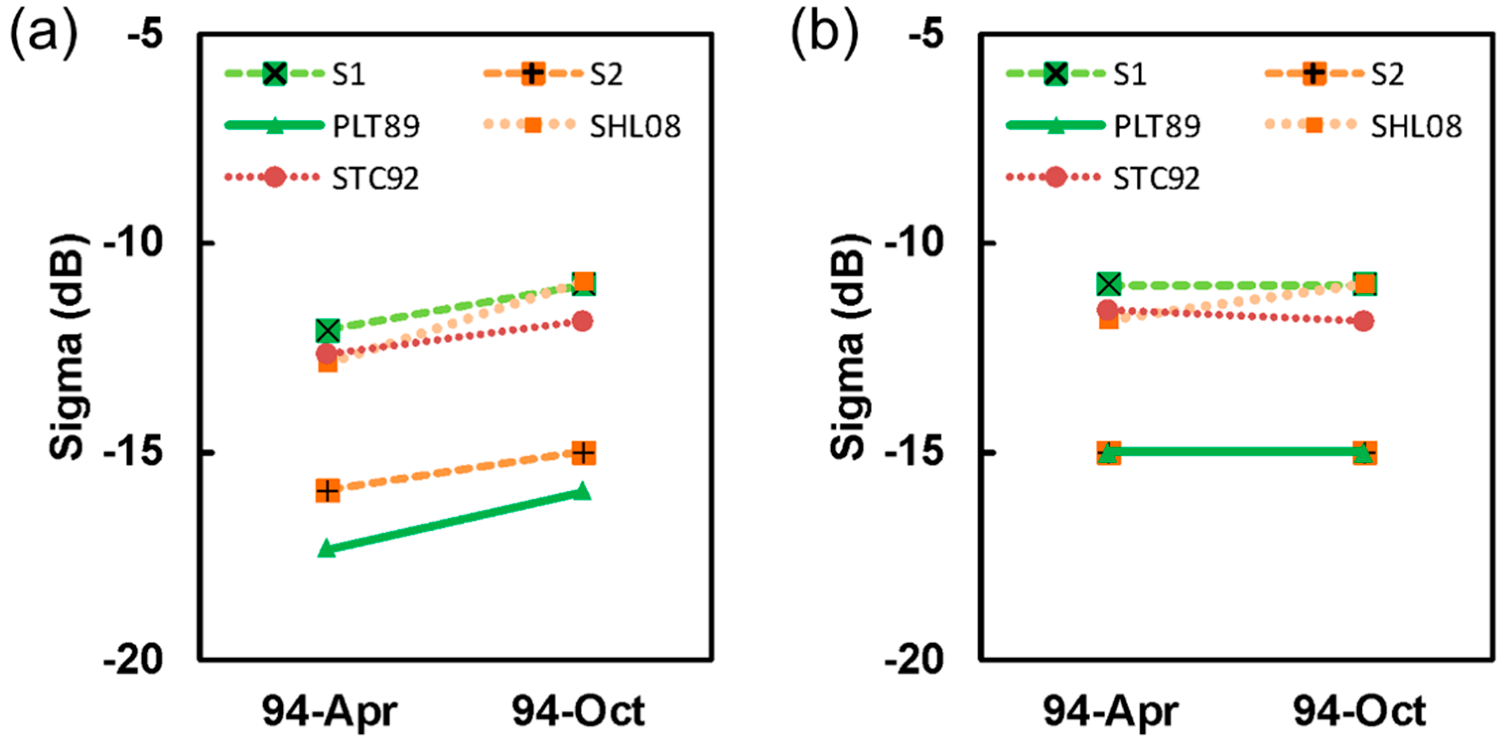
3.3. Sensitivity of SAR Backscatter to Soil Moisture and Cross-Image Normalization
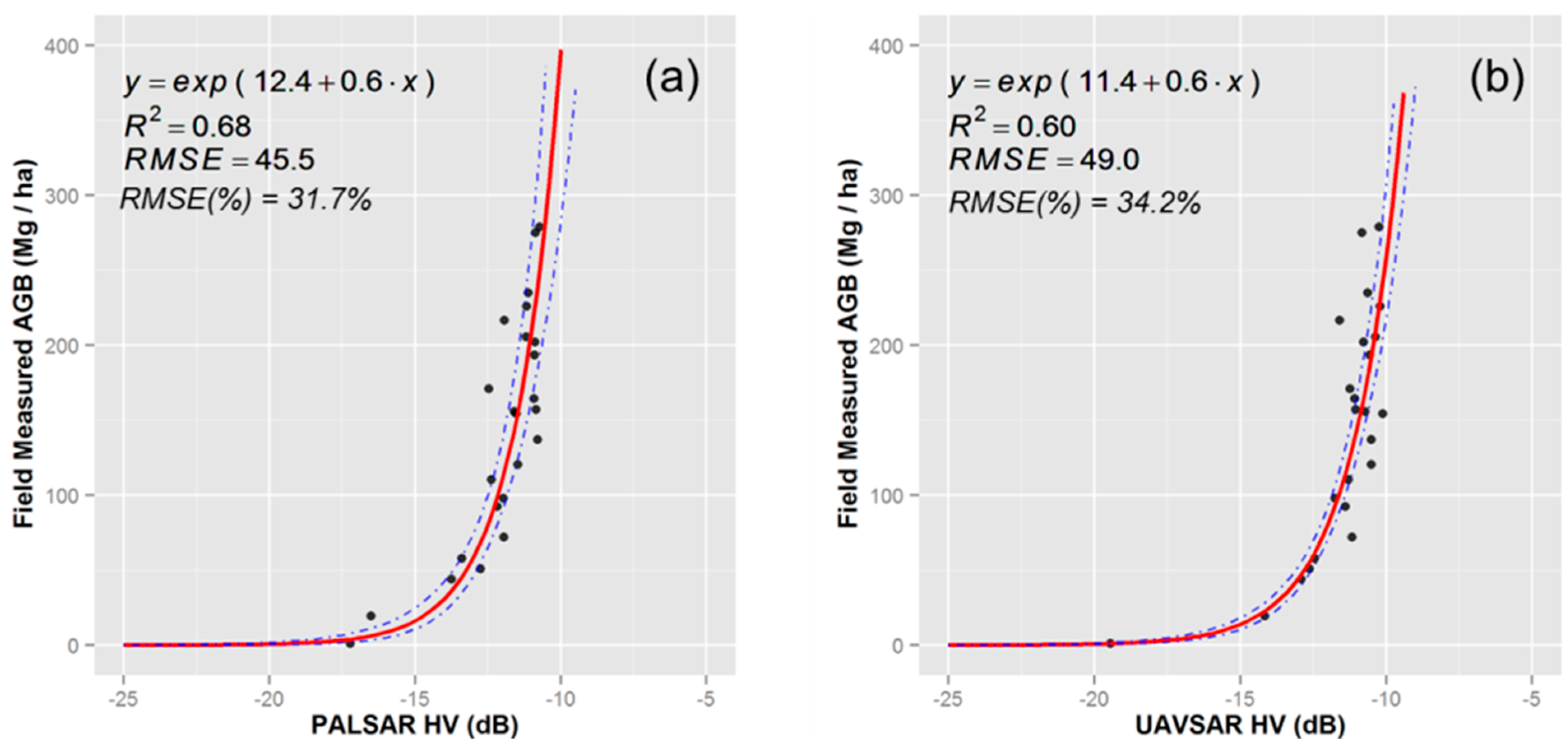
3.4. Regression Model for Forest Biomass Mapping
- (1)
- Select observation i to form a test set (i.e., n independent observations y1, … , yn) and fit the model using the remaining data. Then, compute the predicted residual for the omitted observation:
- (2)
- Repeat step 1 for i = 1, … , n.
- (3)
- Compute the RMSE from , … , , which is called RMSEcv.
4. Results
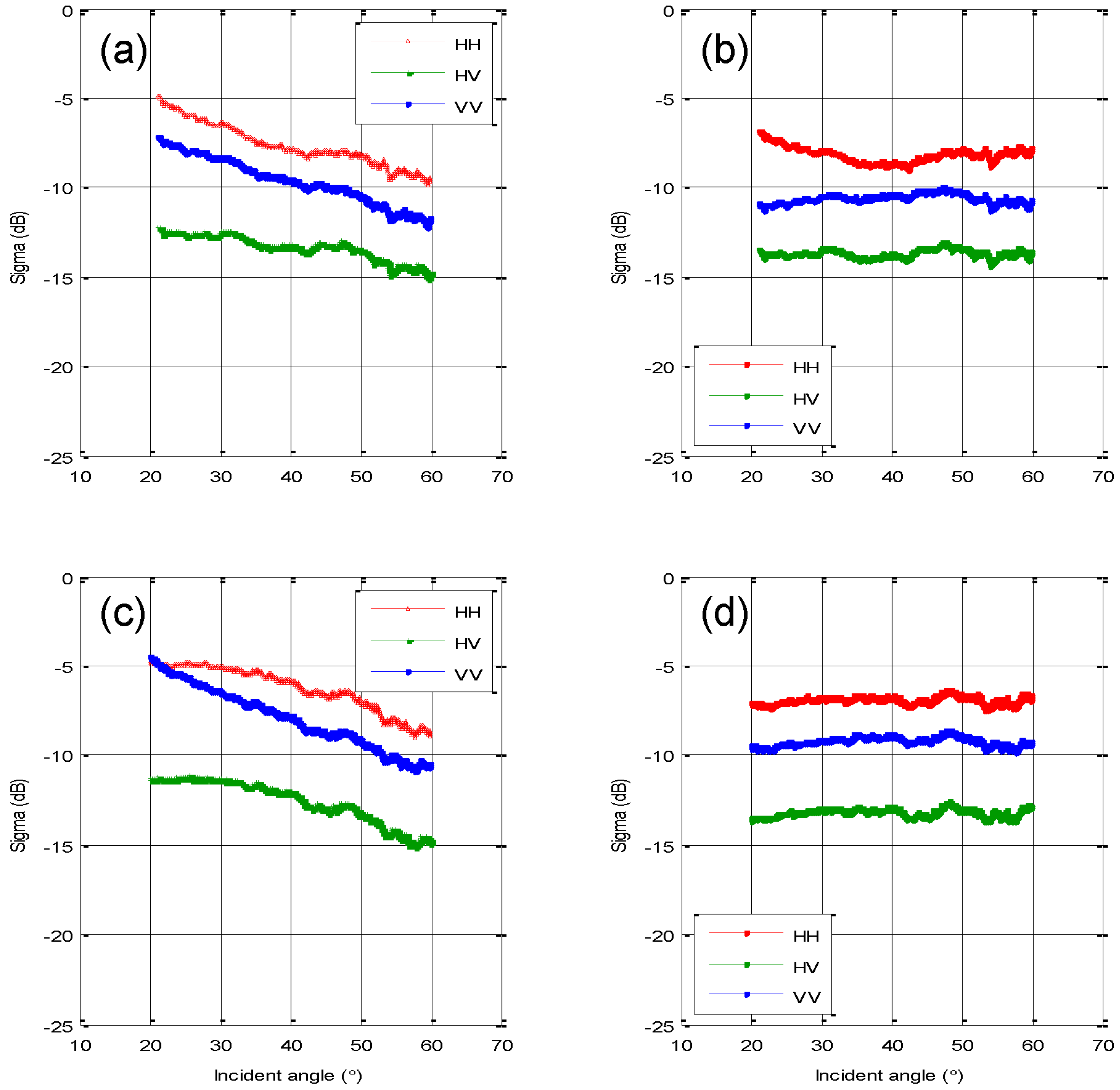
4.1. Sensitivity of SAR Backscatter to Incidence Angle
| Polarization | Correction Model | n | R2 |
|---|---|---|---|
| HH | 1.5940 | 0.9733 | |
| HV | 1.5250 | 0.9665 | |
| VV | −1.3293 | 0.9777 |

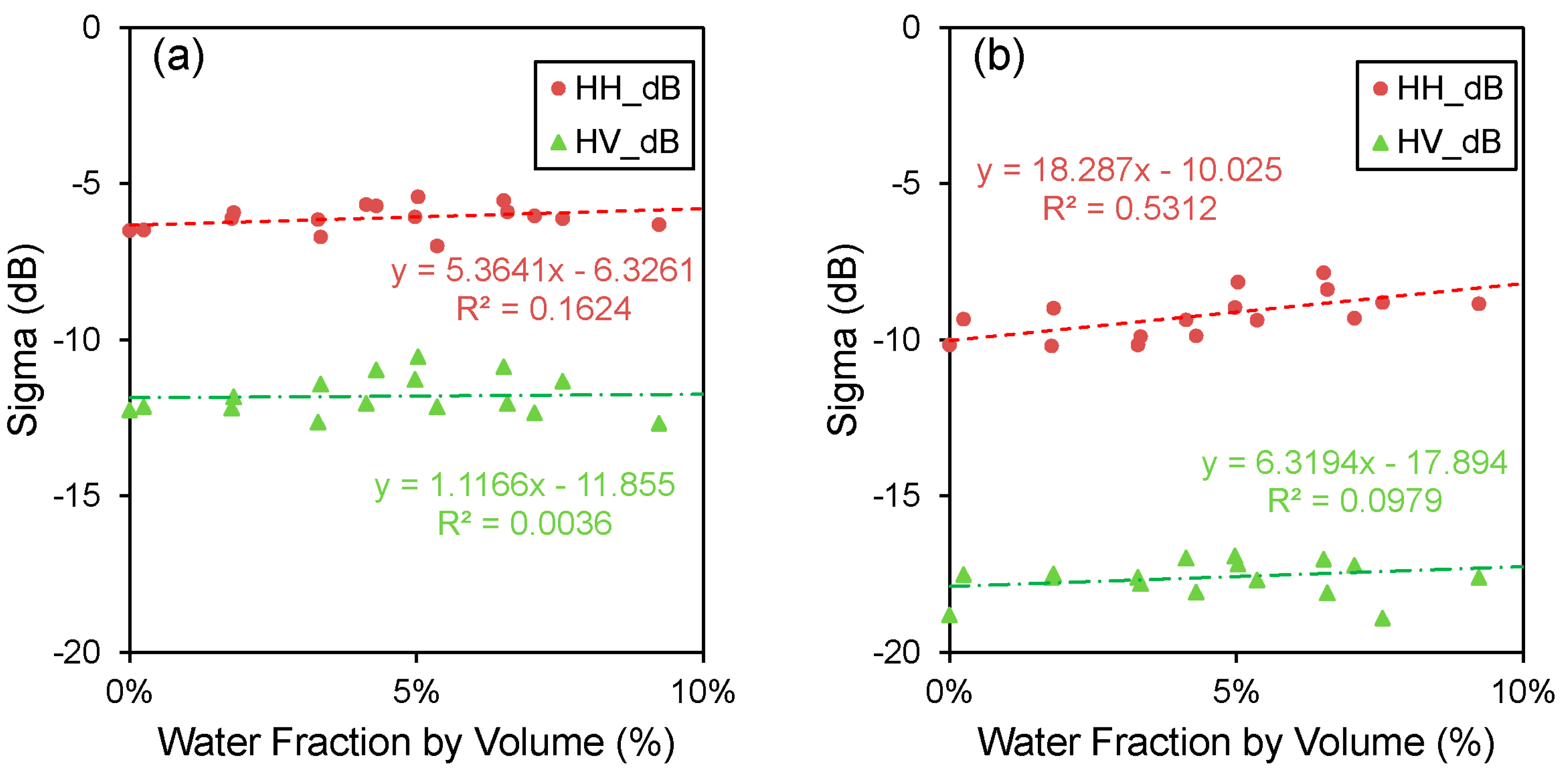
4.2. Sensitivity of SAR Backscatter to Soil Moisture
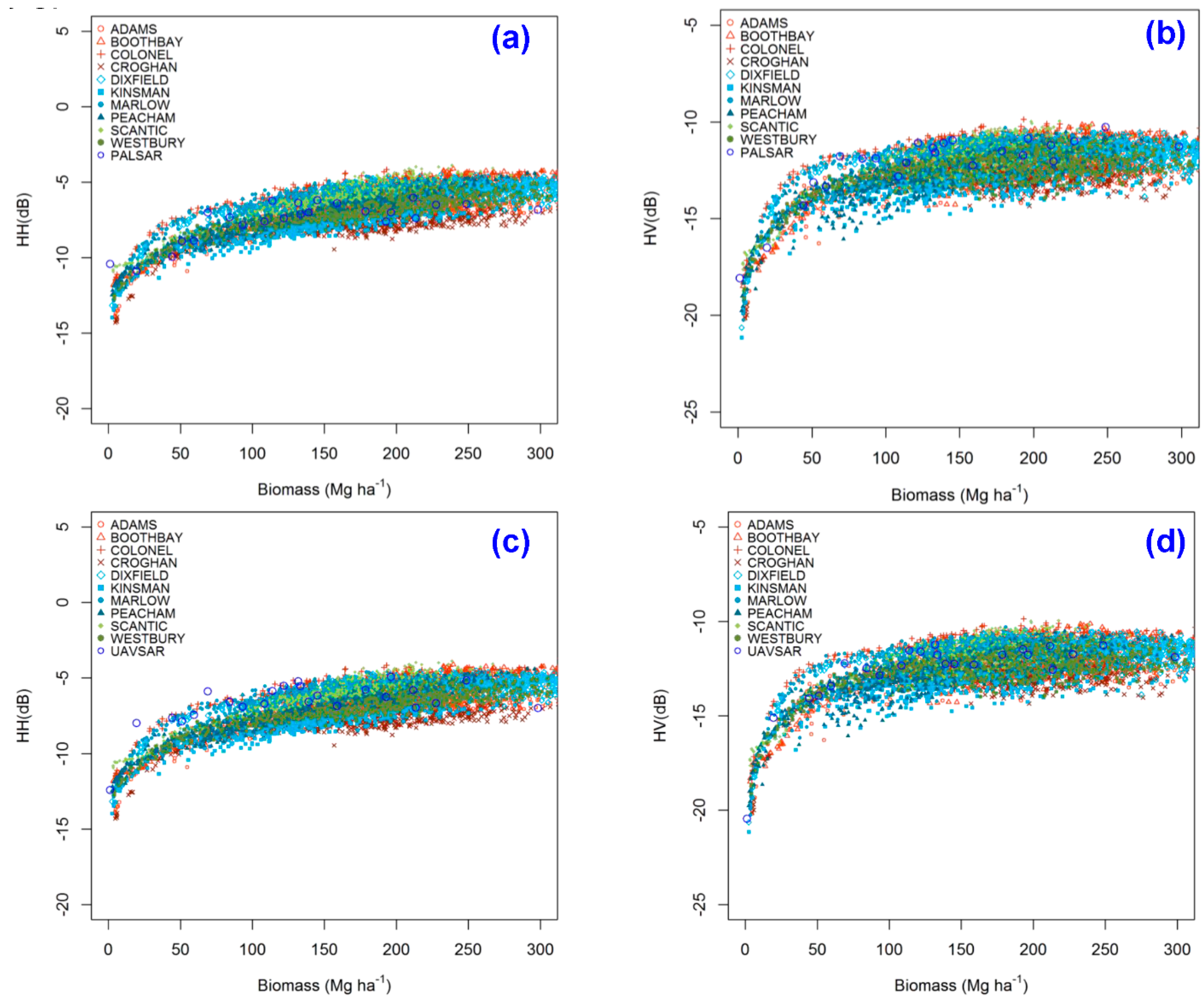
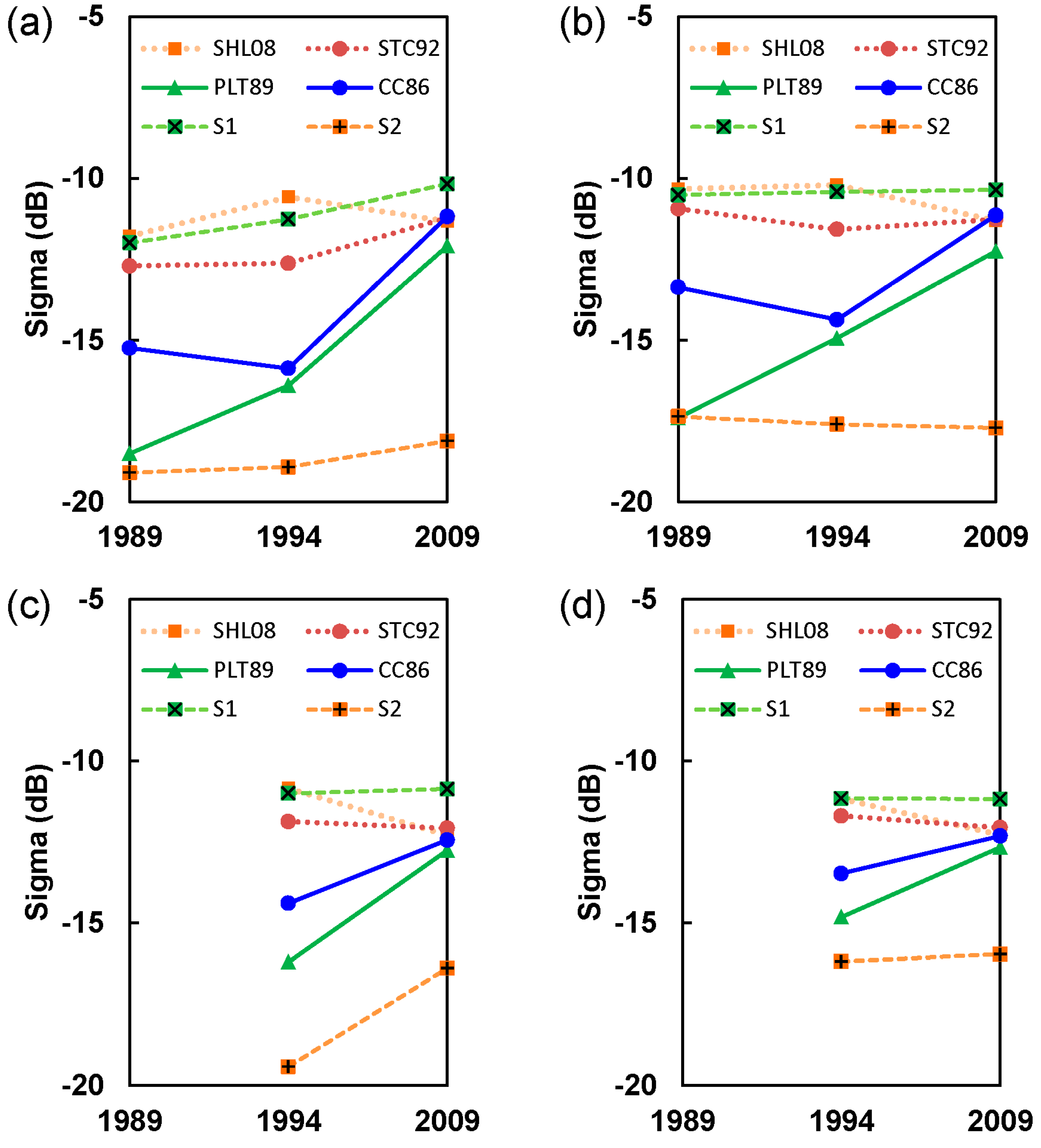
4.3. Sensitivity of Normalized SAR Backscatter to Forest Biomass

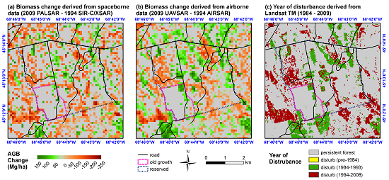
4.4. Mapping Changes of Forest Biomass from SAR Backscatter


5. Discussion
6. Conclusions
Acknowledgments
Author Contributions
Conflicts of Interest
References
- Goetz, S.; Dubayah, R. Advances in remote sensing technology and implications for measuring and monitoring forest carbon stocks and change. Carbon Manag. 2011, 2, 231–244. [Google Scholar] [CrossRef]
- Houghton, R.A.; Hall, F.; Goetz, S.J. Importance of biomass in the global carbon cycle. J. Geophys. Res.: Biogeosci. 2009, 114, G00E03. [Google Scholar] [CrossRef]
- Hall, F.G.; Bergen, K.; Blair, J.B.; Dubayah, R.; Houghton, R.; Hurtt, G.; Kellndorfer, J.; Lefsky, M.; Ranson, J.; Saatchi, S.; et al. Characterizing 3D vegetation structure from space: Mission requirements. Remote Sens. Environ. 2011, 115, 2753–2775. [Google Scholar] [CrossRef]
- Kasischke, E.S.; Melack, J.M.; Craig Dobson, M. The use of imaging radars for ecological applications—A review. Remote Sens. Environ. 1997, 59, 141–156. [Google Scholar] [CrossRef]
- Lu, D. The potential and challenge of remote sensing-based biomass estimation. Int. J. Remote Sens. 2006, 27, 1297–1328. [Google Scholar] [CrossRef]
- Santos, J.R.; Lacruz, M.S.P.; Araujo, L.S.; Keil, M. Savanna and tropical rainforest biomass estimation and spatialization using JERS-1 data. Int. J. Remote Sens. 2002, 23, 1217–1229. [Google Scholar] [CrossRef]
- Collins, J.N.; Hutley, L.B.; Williams, R.J.; Boggs, G.; Bell, D.; Bartolo, R. Estimating landscape-scale vegetation carbon stocks using airborne multi-frequency polarimetric synthetic aperture radar (SAR) in the savannahs of north australia. Int. J. Remote Sens. 2009, 30, 1141–1159. [Google Scholar] [CrossRef]
- Mitchard, E.T.A.; Saatchi, S.S.; Woodhouse, I.H.; Nangendo, G.; Ribeiro, N.S.; Williams, M.; Ryan, C.M.; Lewis, S.L.; Feldpausch, T.R.; Meir, P. Using satellite radar backscatter to predict above-ground woody biomass: A consistent relationship across four different african landscapes. Geophys. Res. Lett. 2009, 36, L23401. [Google Scholar] [CrossRef]
- Ranson, K.J.; Sun, G. Mapping biomass of a northern forest using multifrequency SAR data. IEEE Trans. Geosci. Remote Sens. 1994, 32, 388–396. [Google Scholar] [CrossRef]
- Ranson, K.J.; Saatchi, S.; Guoqing, S. Boreal forest ecosystem characterization with SIR-C/XSAR. IEEE Trans. Geosci. Remote Sens. 1995, 33, 867–876. [Google Scholar] [CrossRef]
- Dobson, M.C.; Ulaby, F.T.; Pierce, L.E.; Sharik, T.L.; Bergen, K.M.; Kellndorfer, J.; Kendra, J.R.; Li, E.; Lin, Y.C.; Nashashibi, A.; et al. Estimation of forest biophysical characteristics in northern michigan with Sir-C/X-Sar. IEEE Trans. Geosci. Remote Sens. 1995, 33, 877–895. [Google Scholar] [CrossRef]
- Sandberg, G.; Ulander, L.M.H.; Fransson, J.E.S.; Holmgren, J.; le Toan, T. L- and P-band backscatter intensity for biomass retrieval in hemiboreal forest. Remote Sens. Environ. 2011, 115, 2874–2886. [Google Scholar] [CrossRef]
- Robinson, C.; Saatchi, S.; Neumann, M.; Gillespie, T. Impacts of spatial variability on aboveground biomass estimation from L-band radar in a temperate forest. Remote Sens. 2013, 5, 1001–1023. [Google Scholar] [CrossRef]
- Luckman, A.; Baker, J.; Kuplich, T.M.; Yanasse, C.D.C.F.; Frery, A.C. A study of the relationship between radar backscatter and regenerating tropical forest biomass for spaceborne SAR instruments. Remote Sens. Environ. 1997, 60, 1–13. [Google Scholar] [CrossRef]
- Balzter, H.; Skinner, L.; Luckman, A.; Brooke, R. Estimation of tree growth in a conifer plantation over 19 years from multi-satellite L-band SAR. Remote Sens. Environ. 2003, 84, 184–191. [Google Scholar] [CrossRef]
- Rowland, C.S.; Balzter, H.; Dawson, T.P.; Luckman, A.; Patenaude, G.; Skinner, L. Airborne SAR monitoring of tree growth in a coniferous plantation. Int. J. Remote Sens. 2008, 29, 3873–3889. [Google Scholar] [CrossRef] [Green Version]
- Santoro, M.; Fransson, J.E.S.; Eriksson, L.E.B.; Ulander, L.M.H. Clear-cut detection in swedish boreal forest using multi-temporal alos PALSAR backscatter data. IEEE J. Sel. Top. Appl. Earth Obs. Remote Sens. 2010, 3, 618–631. [Google Scholar] [CrossRef]
- Sun, G.; Simonett, D.S.; Strahler, A.H. A radar backscatter model for discontinuous coniferous forests. IEEE Trans. Geosci. Remote Sens. 1991, 29, 639–650. [Google Scholar] [CrossRef]
- Wang, Y.; Day, J.L.; Davis, F.W.; Melack, J.M. Modeling L-band radar backscatter of alaskan boreal forest. IEEE Trans. Geosci. Remote Sens. 1993, 31, 1146–1154. [Google Scholar] [CrossRef]
- Sun, G.; Ranson, K.J. Radar modelling of forest spatial patterns. Int. J. Remote Sens. 1998, 19, 1769–1791. [Google Scholar] [CrossRef]
- Harrell, P.A.; Kasischke, E.S.; Bourgeau-Chavez, L.L.; Haney, E.M.; Christensen, N.L., Jr. Evaluation of approaches to estimating aboveground biomass in southern pine forests using SIR-C data. Remote Sens. Environ. 1997, 59, 223–233. [Google Scholar] [CrossRef]
- Kasischke, E.S.; Tanase, M.A.; Bourgeau-Chavez, L.L.; Borr, M. Soil moisture limitations on monitoring boreal forest regrowth using spaceborne L-band SAR data. Remote Sens. Environ. 2011, 115, 227–232. [Google Scholar] [CrossRef]
- Lucas, R.; Armston, J.; Fairfax, R.; Fensham, R.; Accad, A.; Carreiras, J.; Kelley, J.; Bunting, P.; Clewley, D.; Bray, S.; et al. An evaluation of the ALOS PALSAR L-band backscatter—Above ground biomass relationship Queensland, Australia: Impacts of surface moisture condition and vegetation structure. IEEE J. Sel. Top. Appl. Earth Obs. Remote Sens. 2010, 3, 576–593. [Google Scholar] [CrossRef]
- Way, J.; Paris, J.; Dobson, M.C.; McDonals, K.; Ulaby, F.T.; Weber, J.; Ustin, L.; Vanderbilt, V.C.; Kasischke, E.S. Diurnal change in trees as observed by optical and microwave sensors: The EOS synergism study. IEEE Trans.Geosci. Remote Sens. 1991, 29, 807–821. [Google Scholar] [CrossRef]
- Dobson, M.C.; Ulaby, F.T.; LeToan, T.; Beaudoin, A.; Kasischke, E.S.; Christensen, N. Dependence of radar backscatter on coniferous forest biomass. IEEE Trans.Geosci. Remote Sens. 1992, 30, 412–415. [Google Scholar] [CrossRef]
- Ranson, K.J.; Sun, G. An evaluation of AIRSAR and Sir-C/X-Sar images for mapping northern forest attributes in Maine, USA. Remote Sens. Environ. 1997, 59, 203–222. [Google Scholar] [CrossRef]
- Ranson, K.J.; Sun, G. Effects of environmental conditions on boreal forest classification and biomass estimates with SAR. IEEE Trans. Geosci. Remote Sens. 2000, 38, 1242–1252. [Google Scholar] [CrossRef]
- Imhoff, M.L. Radar backscatter and biomass saturation: Ramifications for global biomass inventory. IEEE Trans. Geosci. Remote Sens. 1995, 33, 511–518. [Google Scholar] [CrossRef]
- Zink, M.; Olivier, P.; Freeman, A. Cross-calibration between airborne SAR sensors. IEEE Trans. Geosci. Remote Sens. 1993, 31, 237–245. [Google Scholar] [CrossRef]
- Ustin, S.; Wessman, C.; Curtiss, B.; Kasischke, E.; Way, J.B.; Vanderbilt, V. Opportunities for using the EOS imaging spectrometers and synthetic aperture radar in ecological models. Ecology 1991, 72, 1934–1945. [Google Scholar]
- Sandberg, G.; Ulander, L.M.H.; Wallerman, J.; Fransson, J.E.S. Measurements of forest biomass change using P-band synthetic aperture radar backscatter. IEEE Trans. Geosci. Remote Sens. 2014, 52, 6047–6061. [Google Scholar] [CrossRef]
- Huang, W.; Sun, G.; Dubayah, R.; Cook, B.D.; Montesano, P.M.; Ni, W.; Zhang, Z. Mapping biomass change after forest disturbance: Applying lidar footprint-derived models at key map scales. Remote Sens. Environ. 2013, 134, 319–332. [Google Scholar] [CrossRef]
- Jenkins, J.C.; Chojnacky, D.C.; Heath, L.S.; Birdsey, R.A. National-scale biomass estimators for United States tree species. For. Sci. 2003, 49, 12–35. [Google Scholar]
- Huang, C.; Goward, S.N.; Masek, J.G.; Thomas, N.; Zhu, Z.; Vogelmann, J.E. An automated approach for reconstructing recent forest disturbance history using dense Landsat time series stacks. Remote Sens. Environ. 2010, 114, 183–198. [Google Scholar] [CrossRef]
- Urban, D. A Versatile Model to Simulate Forest Pattern: A User’S Guide to ZELIG Version 1.0; Environmental Sciences Department, The University of Virginia: Charlottesville, VI, USA, 1990. [Google Scholar]
- Levine, E.R.; Knox, R.G.; Lawrence, W.T. Relationships between soil properties and vegetation at the northern experimental forest, Howland, Maine. Remote Sens. Environ. 1994, 47, 231–241. [Google Scholar] [CrossRef]
- Ranson, K.J.; Sun, G.; Knox, R.G.; Levine, E.R.; Weishampel, J.F.; Fifer, S.T. Northern forest ecosystem dynamics using coupled models and remote sensing. Remote Sens. Environ. 2001, 75, 291–302. [Google Scholar] [CrossRef]
- Ni, W.; Sun, G.; Guo, Z.; Zhang, Z.; He, Y.; Huang, W. Retrieval of forest biomass from alos PALSAR data using a lookup table method. IEEE J. Sel. Top. Appl. Earth Obs. Remote Sens. 2013, V6, 875–886. [Google Scholar] [CrossRef]
- Menges, C.; van Zyl, J.; Hill, G.; Ahmad, W. A procedure for the correction of the effect of variation in incidence angle on AIRSAR data. Int. J. Remote Sens. 2001, 22, 829–841. [Google Scholar] [CrossRef]
- Sun, G.; Ranson, K.J.; Kharuk, V.I. Radiometric slope correction for forest biomass estimation from sar data in the western Sayani Mountains, Siberia. Remote Sens. Environ. 2002, 79, 279–287. [Google Scholar] [CrossRef]
- Kuhn, M. Building predictive models in R using the caret package. J. Stat. Softw. 2008, 28, 1–26. [Google Scholar]
- Zhao, K.; Popescu, S. Lidar-based mapping of leaf area index and its use for validating globcarbon satellite LAI product in a temperate forest of the southern USA. Remote Sens. Environ. 2009, 113, 1628–1645. [Google Scholar] [CrossRef]
- Small, D. Flattening gamma: Radiometric terrain correction for SAR imagery. IEEE Trans Geosci. Remote Sens. 2011, 49, 3081–3093. [Google Scholar] [CrossRef]
- Zhang, Z. Biomass Retrieval Based on Lidar and SAR Data. Ph.D. Dissertation, Beijing Normal University, Beijing, China, 2011. [Google Scholar]
- Englhart, S.; Keuck, V.; Siegert, F. Aboveground biomass retrieval in tropical forests—The potential of combined X- and L-band SAR data use. Remote Sens. Environ. 2011, 115, 1260–1271. [Google Scholar] [CrossRef]
© 2015 by the authors; licensee MDPI, Basel, Switzerland. This article is an open access article distributed under the terms and conditions of the Creative Commons Attribution license (http://creativecommons.org/licenses/by/4.0/).
Share and Cite
Huang, W.; Sun, G.; Ni, W.; Zhang, Z.; Dubayah, R. Sensitivity of Multi-Source SAR Backscatter to Changes in Forest Aboveground Biomass. Remote Sens. 2015, 7, 9587-9609. https://doi.org/10.3390/rs70809587
Huang W, Sun G, Ni W, Zhang Z, Dubayah R. Sensitivity of Multi-Source SAR Backscatter to Changes in Forest Aboveground Biomass. Remote Sensing. 2015; 7(8):9587-9609. https://doi.org/10.3390/rs70809587
Chicago/Turabian StyleHuang, Wenli, Guoqing Sun, Wenjian Ni, Zhiyu Zhang, and Ralph Dubayah. 2015. "Sensitivity of Multi-Source SAR Backscatter to Changes in Forest Aboveground Biomass" Remote Sensing 7, no. 8: 9587-9609. https://doi.org/10.3390/rs70809587