
Evaluation of Land Surface Temperature Retrieval from FY-3B/VIRR Data in an Arid Area of Northwestern China


 ,
,  and
and
Abstract
:
1. Introduction
2. Methodology
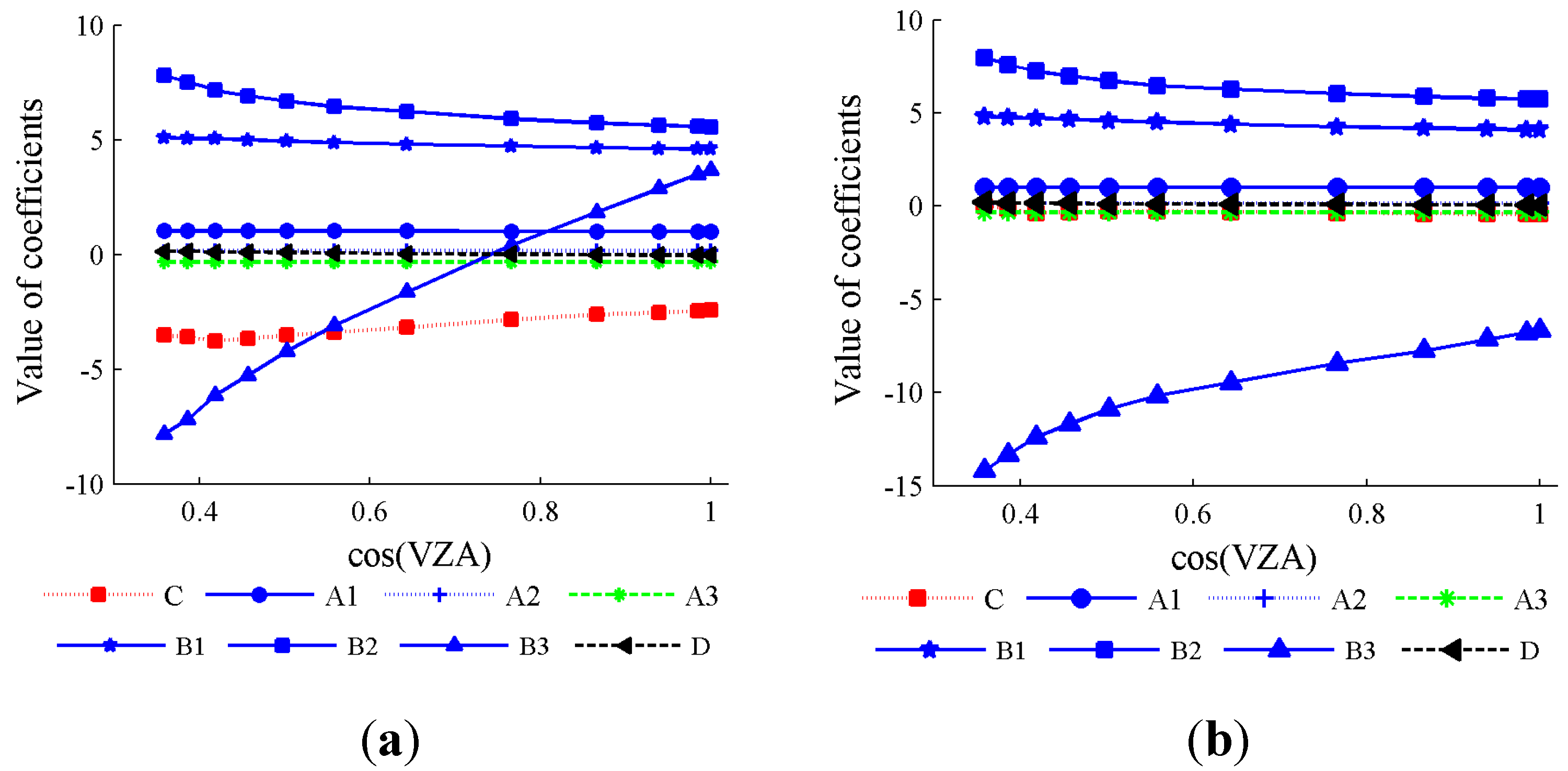
2.1. The GSW Algorithm for FY-3B/VIRR
2.2. Obtaining GSW Algorithm Coefficients

2.3. Sensitivity Analysis
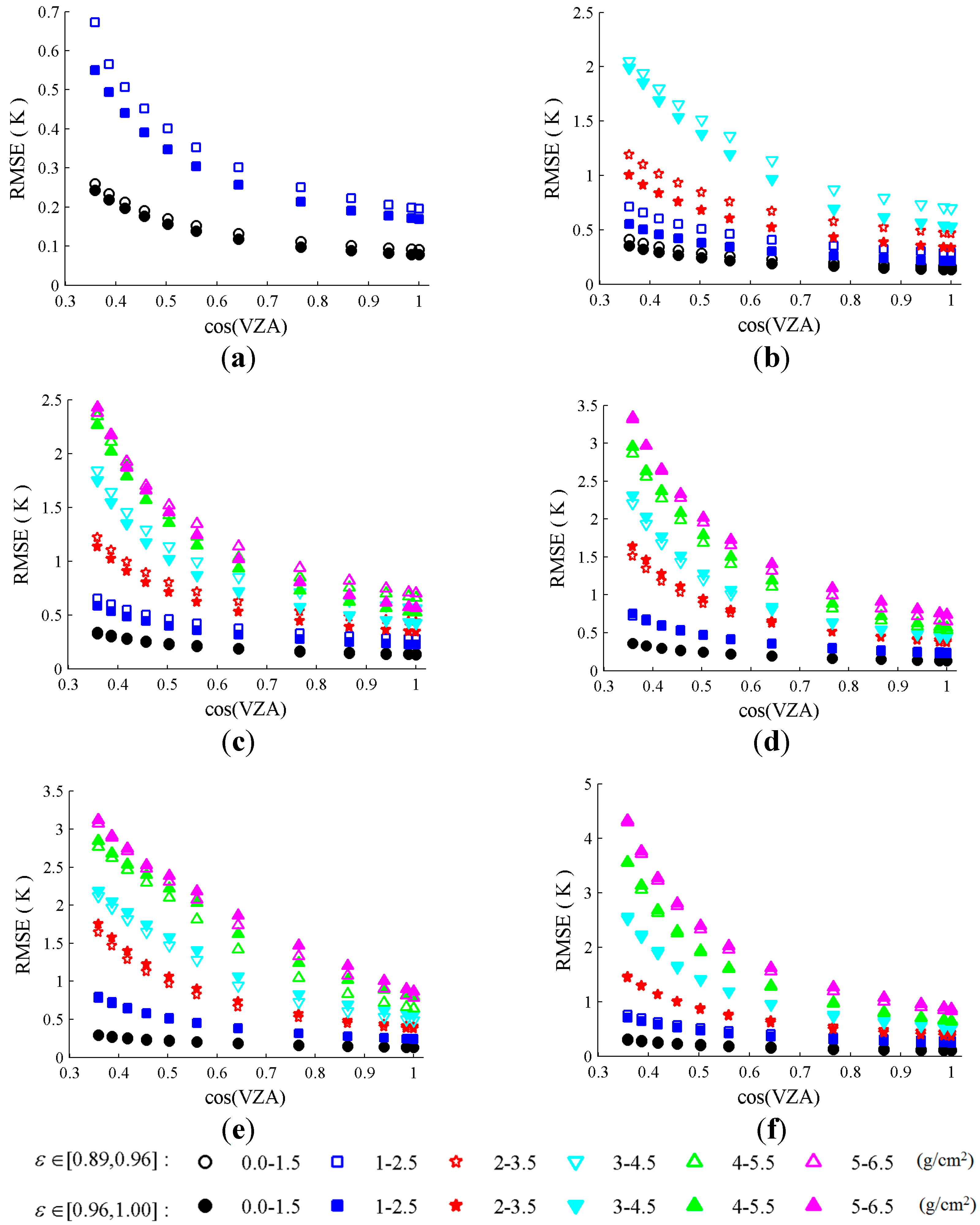
2.3.1. Sensitivity to Brightness Temperatures Uncertainty

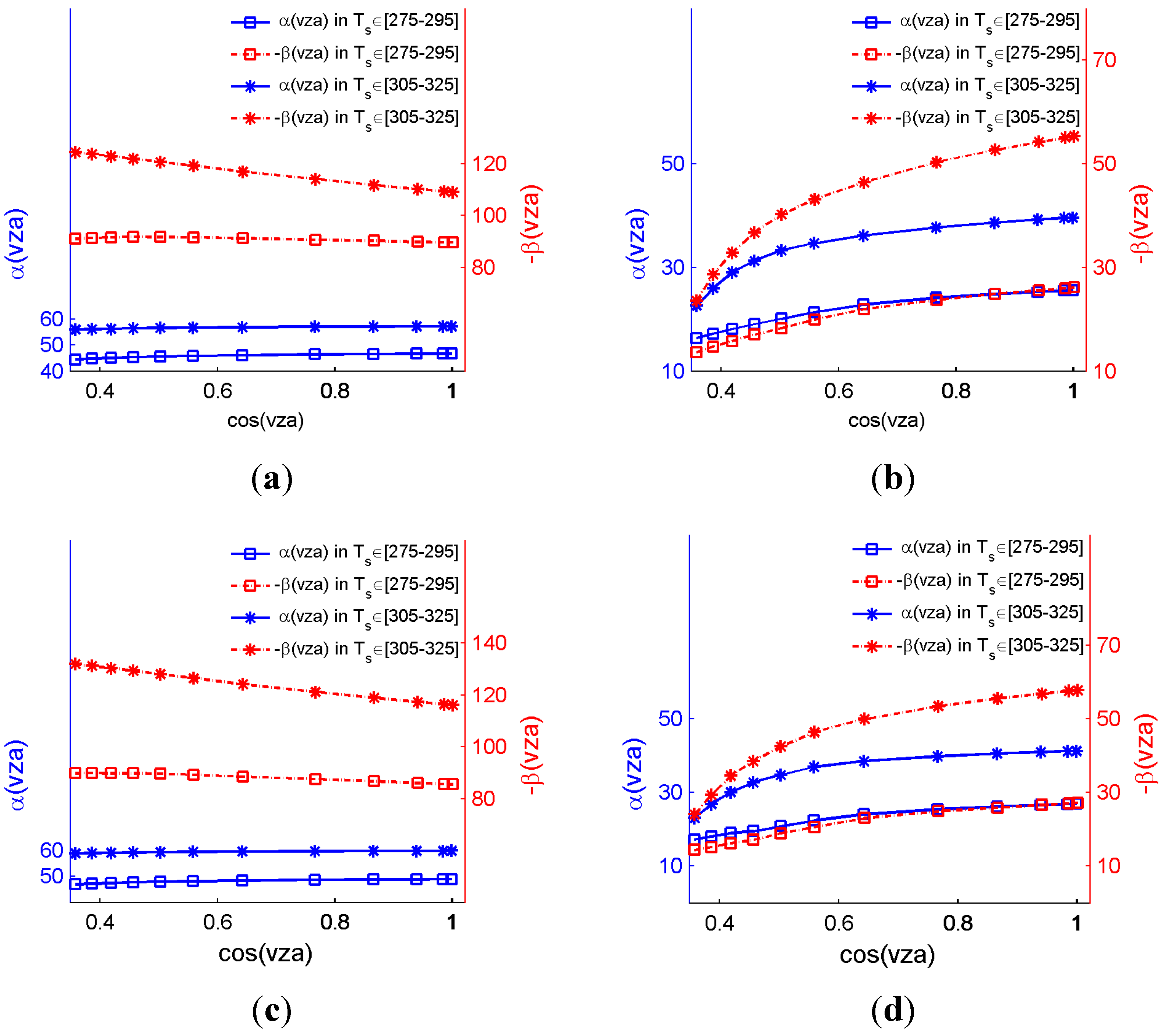
2.3.2. Sensitivity to LSE Uncertainty
- (a)
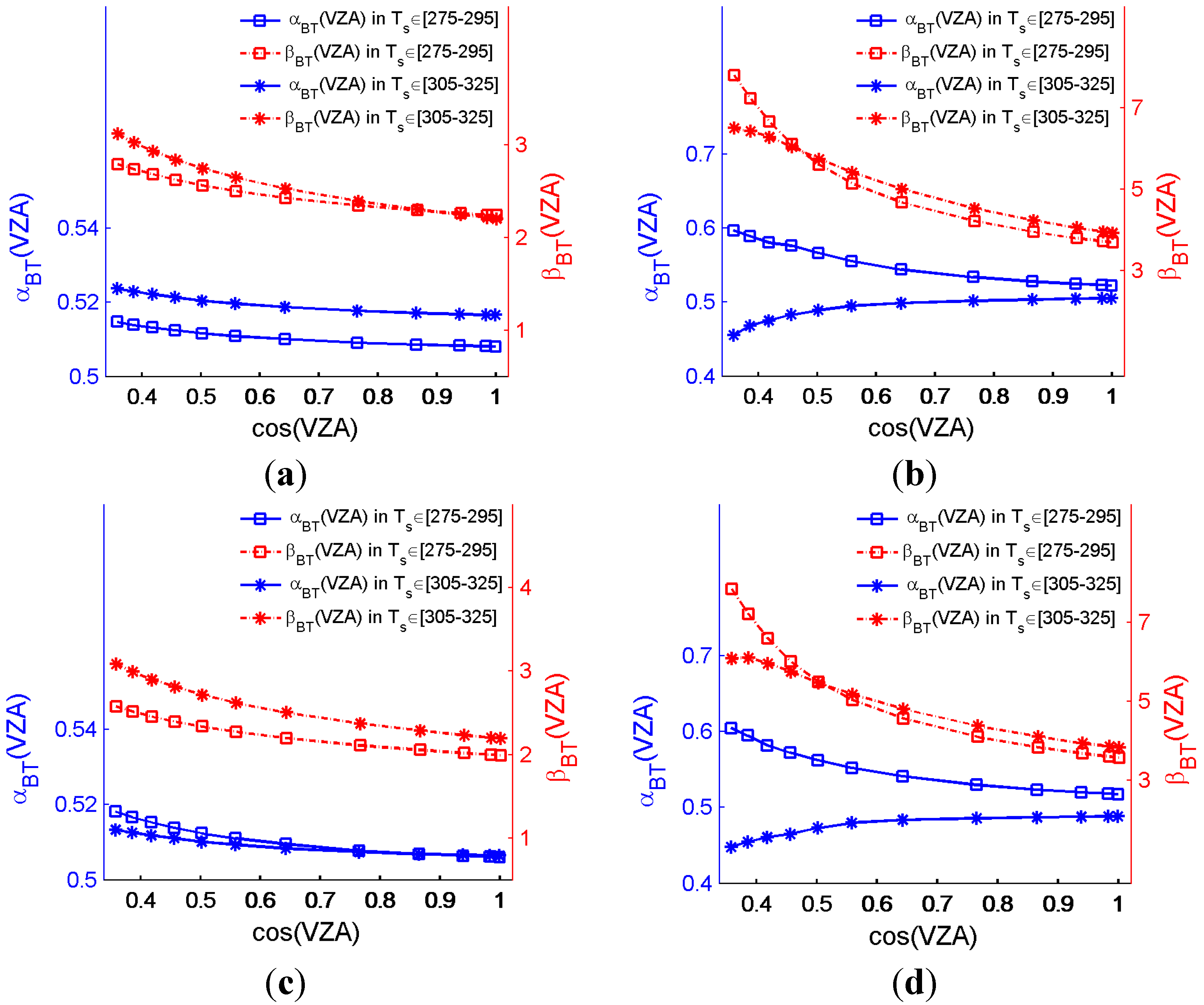
- The values of α and the absolute values of β when LST ϵ [305, 325] K are larger than that those of LST ϵ [275, 295] K for each sub-range, implying that the emissivity sensitivity increases as LST increases, because the emissivity effect is compensated partially by the reflected downward atmospheric radiation.
- (b)
- The absolute values of β are two times greater than α in two LST sub-ranges in dry atmospheric conditions (Figure 5a,c) but are approximately the same in wet atmospheric conditions (Figure 5b,d), indicating that the GSW algorithm is more sensitive to uncertainty in ∆ε in dry atmospheric conditions. This finding is consistent with the emissivity sensitivity analysis for MODIS, where the sensitivity decreases as WVC increases because of the compensative effect of the reflected downward atmospheric thermal infrared radiation [45].
- (c)
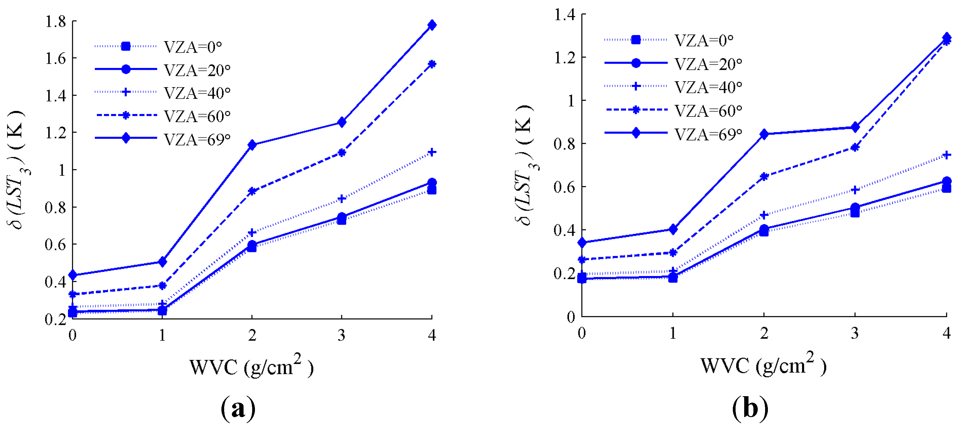
- The value of α (absolute β) at VZA = 0° is approximately two times larger than that at VZA = 69° for a wet atmosphere but is the same for a dry atmosphere, implying that the effect of VZA on both α and β increases from dry to wet atmospheres.
2.3.3. Sensitivity Analysis to Atmospheric WVC
2.3.4. Root Sum Square (RSS) of Uncertainties


| Uncertainties | Viewing Angle | ||||
|---|---|---|---|---|---|
| 0° | 20° | 40° | 60° | 69° | |
| WVC ϵ [0, 1.5], LST ϵ [290, 310], ε ϵ [0.94, 1.00] | |||||
| error in algorithm | 0.13 | 0.14 | 0.16 | 0.23 | 0.33 |
| 0.01 error in (1 − ε)/ε and ∆ε/ε2 | 1.15 | 1.16 | 1.18 | 1.22 | 1.24 |
| error due to ∆T and T45 (0.28 K) | 0.61 | 0.62 | 0.66 | 0.75 | 0.85 |
| ±0.4 g/cm−2 error in WVC | 0.17 | 0.17 | 0.20 | 0.26 | 0.34 |
| RSS (K) | 1.32 | 1.33 | 1.37 | 1.47 | 1.58 |
| WVC ϵ [4, 5.5], LST ϵ [290, 310], ε ϵ [0.94, 1.00] | |||||
| error in algorithm | 0.53 | 0.56 | 0.73 | 1.36 | 2.27 |
| 0.01 error in (1 − ε)/ε and ∆ε/ε2 | 0.52 | 0.52 | 0.48 | 0.39 | 0.24 |
| error due to ∆T and T45 (0.28 K) | 1.04 | 1.07 | 1.19 | 1.54 | 1.75 |
| 10% error in WVC | 0.59 | 0.63 | 0.75 | 1.27 | 1.29 |
| RSS (K) | 1.41 | 1.46 | 1.66 | 2.44 | 3.15 |
3. Evaluation with Ground-Measured LST
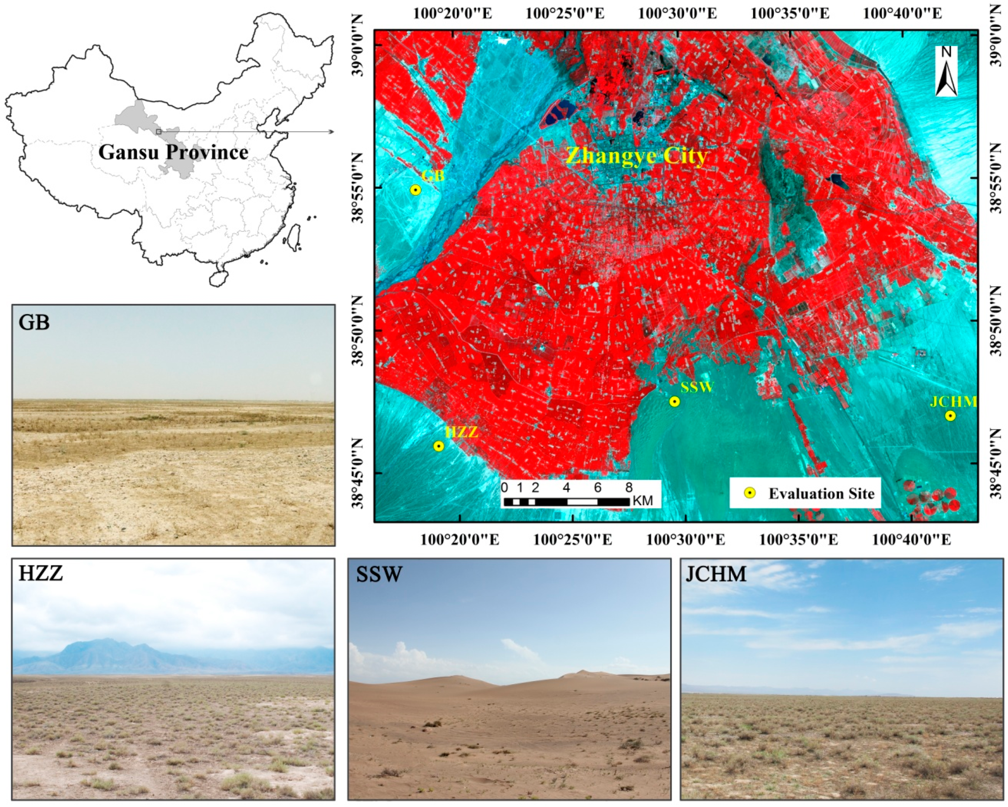
3.1. Study Area and Datasets

| Site | Latitude/Longitude | Elevation (m) | Land Cover | Land Cover type | Radiometers | Time Period (year/month/day) | |
|---|---|---|---|---|---|---|---|
| VIRR | MODIS_IGBP | ||||||
| GB | 38.9150°N 100.3042°E | 1567 | Gobi | 7, 16 | 10 | CNR1 | 2012/08/01–2013/12/31 |
| SSW | 38.7892°N 100.4933°E | 1555 | Sand dune | 16 | 10 | CNR1 | 2012/06/08–2013/12/31 |
| HZZ | 38.7652°N 100.3186°E | 1735 | Desert steppe | 7, 16, 10 | 10 | SI-111 | 2012/06/04–2013/12/31 |
| JCHM | 38.7781°N 100.6967°E | 1625 | Desert steppe | 16 | 10 | SI-111 | 2012/06/29–2013/12/31 |
3.2. Ground-Measured LST Estimation
3.3. The LST Retrieval
3.3.1. Calculations of LSE
| Site | εAG1km | ΔεAG1km | ε2012 | Δε2012 | εspec. | Δεspec. |
|---|---|---|---|---|---|---|
| GB | 0.966 | −0.009 | 0.966 | −0.010 | 0.971 | −0.009 |
| SSW | 0.955 | −0.018 | 0.957 | −0.019 | 0.971 | −0.009 |
| HZZ | 0.971 | −0.005 | 0.975 | −0.006 | 0.971 | −0.009 |
| JCHM | 0.967 | −0.008 | 0.975 | −0.006 | 0.971 | −0.009 |
3.3.2. Determination of the TOA BT
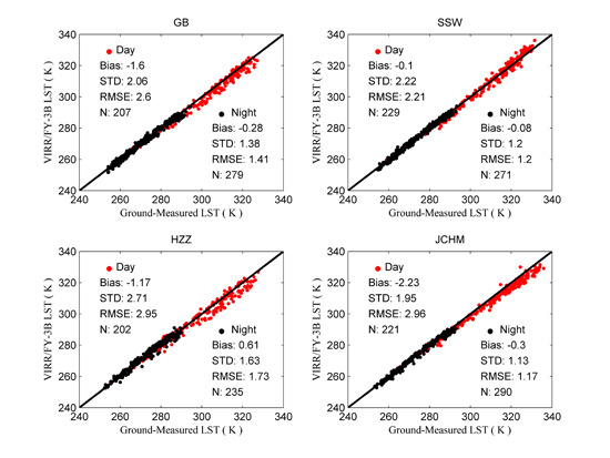
3.4. Results and Discussion
| Site | Bias | STD | RMSE | N | ||||||
|---|---|---|---|---|---|---|---|---|---|---|
| TAG1km − Tg | T2012 − Tg | TSpec − Tg | TAG1km − Tg | T2012 − Tg | TSpec − Tg | TAG1km − Tg | T2012 − Tg | TSpec − Tg | ||
| GB | −0.28 | −0.17 | −0.47 | 1.38 | 1.38 | 1.38 | 1.41 | 1.38 | 1.45 | 279 |
| SSW | −0.08 | −0.08 | −1.77 | 1.20 | 1.20 | 1.21 | 1.20 | 1.20 | 2.14 | 271 |
| HZZ | 0.61 | 0.54 | 1.08 | 1.63 | 1.62 | 1.62 | 1.73 | 1.71 | 1.94 | 235 |
| JCHM | −0.30 | −0.84 | −0.31 | 1.13 | 1.13 | 1.13 | 1.17 | 1.41 | 1.17 | 290 |
| ALL | −0.04 | −0.17 | −0.41 | 1.38 | 1.42 | 1.65 | 1.38 | 1.43 | 1.70 | 1075 |
| Site | Bias | STD | RMSE | N | ||||||
|---|---|---|---|---|---|---|---|---|---|---|
| TAG1km − Tg | T2012 − Tg | TSpec − Tg | TAG1km − Tg | T2012 − Tg | TSpec − Tg | TAG1km − Tg | T2012 − Tg | TSpec − Tg | ||
| GB | −1.60 | −1.50 | −1.85 | 2.06 | 2.06 | 2.06 | 2.60 | 2.54 | 2.76 | 207 |
| SSW | −0.10 | −0.12 | −2.05 | 2.22 | 2.22 | 2.10 | 2.21 | 2.21 | 2.93 | 229 |
| HZZ | −1.17 | −1.28 | −0.70 | 2.71 | 2.71 | 2.70 | 2.95 | 2.99 | 2.78 | 202 |
| JCHM | −2.23 | −2.89 | −2.28 | 1.95 | 1.99 | 1.95 | 2.96 | 3.51 | 3.00 | 221 |
| ALL | −1.26 | −1.44 | −1.74 | 2.38 | 2.47 | 2.29 | 2.69 | 2.85 | 2.87 | 859 |

| Site | Bias | Std |
|---|---|---|
| GB | 16.81 | 3.30 |
| SSW | 21.62 | 2.91 |
| HZZ | 19.86 | 5.83 |

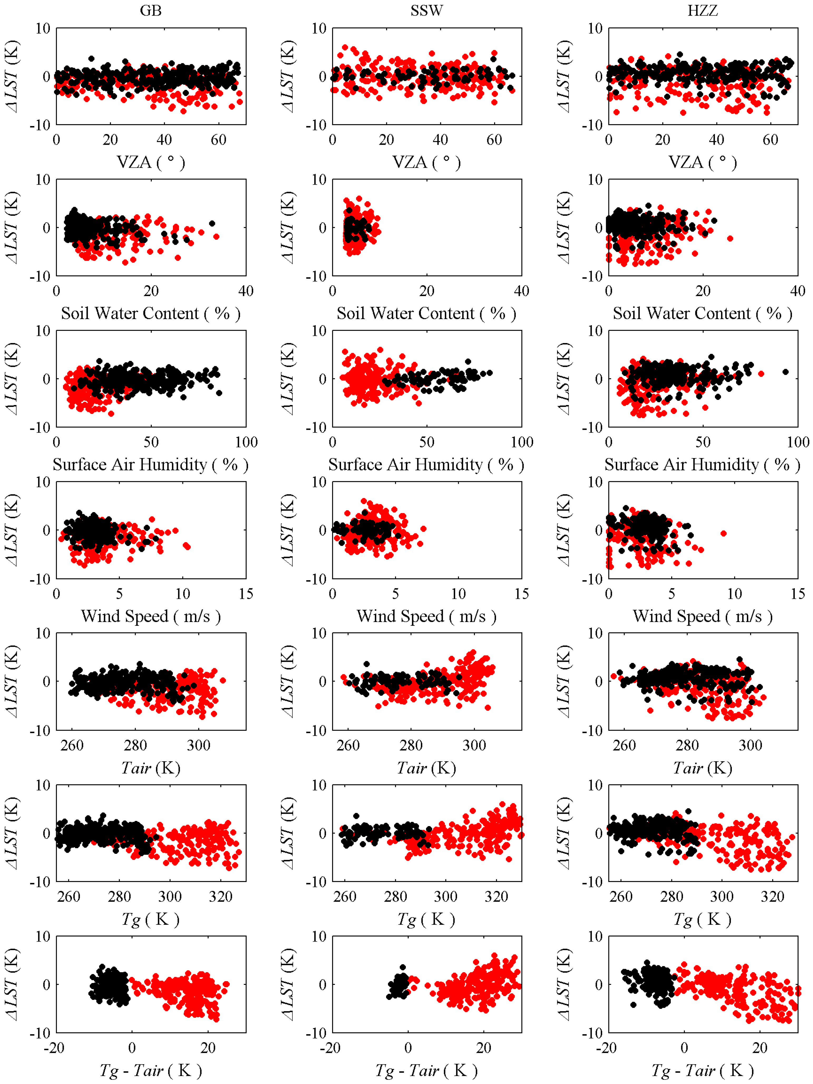
| Variable | All | GB | SSW | HZZ | ||||
|---|---|---|---|---|---|---|---|---|
| R2 | R2 | R2 | R2 | |||||
| Daytime | Nighttime | Daytime | Nighttime | Daytime | Nighttime | Daytime | Nighttime | |
| VZA | 0.010 | 0.002 | 0.050 | 0.009 | 0.009 | 0.006 | 0.015 | 0 |
| Soil Water Content | 0 | 0.013 | 0 | 0.021 | 0 | 0.001 | 0.055 | 0.003 |
| Surface Air Humidity | 0.013 | 0 | 0.015 | 0.002 | 0.002 | 0.099 | 0.030 | 0.004 |
| Wind Speed | 0.013 | 0 | 0.007 | 0.036 | 0.015 | 0.013 | 0.029 | 0.004 |
| Tair | 0.012 | 0 | 0.003 | 0.004 | 0.208 | 0.001 | 0.028 | 0.004 |
| Tg | 0.073 | 0.002 | 0.016 | 0.002 | 0.193 | 0.004 | 0.201 | 0.002 |
| Tg − Tair | 0.014 | 0.002 | 0.063 | 0.009 | 0.121 | 0.006 | 0.030 | 0 |
4. Conclusions
Acknowledgments
Author Contributions
Conflicts of Interest
References
- Camillo, P.J. Using one- or two-layer models for evaporation estimation with remotely sensed data. In Land Surface Evaporation, Measurements and Parameterization; Schmugge, T.J., André, J.C., Eds.; Springer New York: New York, NY, USA, 1991; pp. 183–197. [Google Scholar]
- Schmugge, T.J.; Becker, F.; Li, Z.L. Spectral emissivity variations in airborne surface temperature measurements. Remote Sens. Environ. 1991, 35, 95–104. [Google Scholar] [CrossRef]
- Zhang, L.; Lemeur, R.; Goutorbec, J.P. A one-layer resistance model for estimating regional evapotranpiration using remote sensing data. Agric. For. Meteorol. 1995, 77, 241–261. [Google Scholar] [CrossRef]
- Anderson, M.C.; Norman, J.M.; Diak, G.R.; Mecikalski, J.R. A two-source time-integrated model for estimating surface fluxes using thermal infrared remote sensing. Remote Sens. Environ. 1997, 60, 195–216. [Google Scholar] [CrossRef]
- Su, Z. The surface energy balance system (SEBS) for estimation of turbulent heat fluxes. Hydrol. Earth Syst. Sci. 2002, 6, 85–100. [Google Scholar] [CrossRef]
- Weng, Q.H.; Lu, D.S.; Schubring, J. Estimation of land surface temperature-vegetation abundance relationship for urban heat island studies. Remote Sens. Environ. 2004, 89, 467–483. [Google Scholar] [CrossRef]
- Zhou, L.; Dickinson, R.E.; Tian, Y.; Jin, M.; Ogawa, K.; Yu, H.; Schmugge, T. A sensitivity study of climate and energy balance simulations with use of satellite-derived emissivity data over Northern Africa and the Arabian Peninsula. J. Geophys. Res. 2003, 108. [Google Scholar] [CrossRef]
- Kustas, W.; Anderson, M. Advances in thermal infrared remote sensing for land surface modeling. Agric. For. Meteorol. 2009, 149, 2071–2081. [Google Scholar] [CrossRef]
- Anderson, M.C.; Hain, C.R.; Wardlow, B.; Mecikalski, J.R.; Kustas, W.P. Evaluation of a drought index based on thermal remote sensing of evapotranspiration over the continental U.S. J. Clim. 2011, 24, 2025–2044. [Google Scholar] [CrossRef]
- Anderson, M.C.; Allen, R.G.; Morse, A.; Kustas, W.P. Use of Landsat thermal imagery in monitoring evapotranspiration and managing water resources. Remote Sens. Environ. 2012, 122, 50–65. [Google Scholar] [CrossRef]
- Li, Z.L.; Tang, B.H.; Wu, H.; Ren, H.Z.; Yan, G.J.; Wan, Z.M.; Trigo, I.F.; Sobrino, J.A. Satellite-derived land surface temperature: Current status and perspectives. Remote Sens. Environ. 2013, 131, 14–37. [Google Scholar] [CrossRef]
- Liu, Y.; Hiyama, T.; Yamaguchi, Y. Scaling of land surface temperature using satellite data: A case examination on ASTER and MODIS products over a heterogeneous terrain area. Remote Sens. Environ. 2006, 105, 115–128. [Google Scholar] [CrossRef]
- Neteler, M. Estimating daily land surface temperatures in mountainous environments by reconstructed MODIS LST data. Remote Sens. 2010, 2, 333–351. [Google Scholar] [CrossRef]
- Wan, Z.; Dozier, J.A. Generalized split-window algorithm for retrieving land-surface temperature from space. IEEE Trans. Geosci. Remote Sens. 1996, 34, 892–905. [Google Scholar]
- Dash, P.; Gfttsche, F.M.; Olesen, F.S.; Fischer, H. Land surface temperature and emissivity estimation from passive sensor data: Theory and practice-current trends. Int. J. Remote Sens. 2002, 23, 2563–2594. [Google Scholar] [CrossRef]
- Prata, A.J.; Caselles, V.; Coll, C.; Sobrino, J.A.; Ottlé, C. Thermal remote sensing of land surface temperature from satellites: Current status and future prospects. Remote Sens. Rev. 1995, 12, 175–224. [Google Scholar] [CrossRef]
- Anding, D.; Kauth, R. Estimation of sea surface temperatures from space. Remote Sens. Environ. 1970, 1, 217–220. [Google Scholar] [CrossRef]
- Price, J.C. Land surface temperature measurements from the split window channels of the NOAA 7 AVHRR. J. Geophys. Res. 1984, 89, 7231–7237. [Google Scholar] [CrossRef]
- Kerr, Y.H.; Lagouarde, J.P.; Imbernon, J. Accurate land surface temperature retrieval from AVHRR data with use of an improved split window algorithm. Remote Sens. Environ. 1992, 41, 197–209. [Google Scholar] [CrossRef]
- Pinheiro, A.C.T.; Privette, J.L.; Mahoney, R.; Tucker, C.J. Directional effects in a daily AVHRR land surface temperature dataset over Africa. IEEE Trans. Geosci. Remote Sens. 2004, 42, 1941–1954. [Google Scholar] [CrossRef]
- Wan, Z. New refinements and validation of the MODIS land-surface temperature/emissivity products. Remote Sens. Environ. 2008, 112, 59–74. [Google Scholar] [CrossRef]
- Wan, Z. New refinements and validation of the collection-6 MODIS land-surface temperature/emissivity product. Remote Sens. Environ. 2014, 140, 36–45. [Google Scholar] [CrossRef]
- Rozenstein, O.; Qin, Z.; Derimian, Y.; Karnieli, A. Derivation of land surface temperature for Landsat-8 TIRS using a split window algorithm. Sensors 2014, 14, 5768–5780. [Google Scholar] [CrossRef] [PubMed]
- Du, C.; Ren, H.Z.; Qin, Q.M.; Meng, J.J.; Zhao, S.H. A practical split-window algorithm for estimating land surface temperature from landsat 8 Data. Remote Sens. 2015, 7, 647–665. [Google Scholar] [CrossRef]
- Jiang, J.; Liu, Q.; Li, H.; Huang, H. Split-window method for land surface temperature estimation from FY-3A/VIRR data. In Proceedings of the International Symposium on Remote Sensing Environ (IGARSS), Vancouver, BC, Canada, 24–29 July 2011; pp. 305–308.
- Jiang, G.M. Development of split-window algorithm for land surface temperature estimation from the VIRR/FY-3A measurements. IEEE Geosci. Remote Sens. Lett. 2013, 10, 952–956. [Google Scholar] [CrossRef]
- Tang, B.H.; Shao, K.; Li, Z.L.; Wu, H.; Nerry, F.; Zhou, G. Estimation and validation of land surface temperatures from Chinese second-generation polar-orbit FY-3A VIRR data. Remote Sens. 2015, 3250, 3250–3273. [Google Scholar] [CrossRef]
- Trigo, I.F.; Peres, L.F.; DaCamara, C.C.; Freitas, S.C. Thermal land surface emissivity retrieved from SEVIRI/Meteosat. IEEE Trans. Geosci. Remote Sens. 2008, 46, 307–315. [Google Scholar] [CrossRef]
- Jiang, G.M.; Li, Z.L. Split-window algorithm for land surface temperature estimation from MSG1-SEVIRI data. Int. J. Remote Sens. 2008, 29, 6067–6074. [Google Scholar] [CrossRef]
- Gao, C.X.; Tang, B.H.; Wu, H.; Jiang, X.G.; Li, Z.L. A generalized split-window algorithm for land surface temperature estimation from MSG-2/SEVIRI data. Int. J. Remote Sens. 2013, 34, 4182–4199. [Google Scholar] [CrossRef]
- Coll, C.; Valor, E.; Galve, J.M.; Mira, M.; Bisquert, M.; García-Santos, V.; Caselles, E.; Caselles, V. Long-term accuracy assessment of land surface temperatures derived from the Advanced Along-Track Scanning Radiometer. Remote Sens. Environ. 2012, 116, 211–225. [Google Scholar] [CrossRef]
- Sun, D.; Yu, Y.; Fang, L.; Liu, Y. Toward an operational land surface temperature algorithm for GOES. J. Appl. Meteor. Climatol. 2013, 52, 1974–1986. [Google Scholar] [CrossRef]
- Tang, B.H.; Bi, Y.Y.; Li, Z.L.; Xia, J. Generalized split-window algorithm for estimate of land surface temperature from Chinese geostationary FengYun meteorological satellite (FY-2C) data. Sensors 2008, 8, 933–951. [Google Scholar] [CrossRef]
- Wan, Z.; Zhang, Y.; Zhang, Q.; Li, Z.L. Validation of the land-surface temperature products retrieved from Terra Moderate Resolution Imaging Spectroradiometer data. Remote Sens. Environ. 2002, 83, 163–180. [Google Scholar] [CrossRef]
- Wan, Z.; Zhang, Y.; Zhang, Q.; Li, Z.L. Quality assessment and validation of the MODIS global land surface temperature. Int. J. Remote Sens. 2004, 25, 261–274. [Google Scholar] [CrossRef]
- Wan, Z.; Li, Z.L. Radiance-based validation of the V5 MODIS land-surface temperature product. Int. J. Remote Sens. 2008, 29, 5373–5395. [Google Scholar] [CrossRef]
- Li, H.; Sun, D.; Yu, Y.; Wang, H.; Liu, Y.; Liu, Q.; Du, Y.; Wang, H.; Cao, B. Evaluation of the VIIRS and MODIS LST products in an arid area of Northwest China. Remote Sens. Environ. 2014, 142, 111–121. [Google Scholar] [CrossRef]
- Li, X.; Cheng, G.; Liu, S.; Xiao, Q.; Ma, M.; Jin, R.; Che, T.; Liu, Q.; Wang, W.; Qi, Y.; et al. Heihe watershed allied telemetry experimental research (HiWATER): Scientific objectives and experimental design. Bull. Am. Meteorol. Soc. 2013, 94, 1145–1160. [Google Scholar] [CrossRef]
- Guillevic, P.C.; Biard, J.C.; Hulley, G.C.; Privette, J.L.; Hook, S.J.; Olioso, A.; Göttsche, F.M.; Radocinski, R.; Román, M.O.; Yu, Y.; Csiszar, I. Validation of Land Surface Temperature products derived from the Visible Infrared Imaging Radiometer Suite (VIIRS) using ground-based and heritage satellite measurements. Remote Sens. Environ. 2014, 154, 19–37. [Google Scholar] [CrossRef]
- Coll, C.; Caselles, C.; Sobrino, J.A.; Valor, E. On the atmospheric dependence of the split-window equation for land surface temperature. Int. J. Remote Sens. 1994, 15, 1915–1932. [Google Scholar] [CrossRef]
- Li, Z.L.; Petitcolin, F.; Zhang, R.H. A physically based algorithm for land surface emissivity retrieval from combined mid-infrared and thermal infrared data. Sci. China (Ser. E) 2000, 43, 23–33. [Google Scholar] [CrossRef]
- Berk, A.; Bernstein, L.S.; Anderson, G.P.; Acharya, P.K.; Robertson, D.C. MODTRAN cloud and multiple scattering upgrades wit application to AVIRIS. Remote Sens. Environ. 1998, 65, 367–375. [Google Scholar] [CrossRef]
- Atmospheric Radiation Analysis Laboratoire de Météorologie Dynamique/CNRS/IPSL. Available online: http://ara.abct.lmd.polytechnique.fr/index.php?page=tigr (accessed on 1 December 2010).
- Kondratyev, K.Y. Radiation in the Atmosphere, 1st ed.; Academic Press: New York, NY, USA, 1969; p. 911. [Google Scholar]
- Wan, Z. MODIS Land-Surface Temperature Algorithm Theoretical Basis Document (LST ATBD), Version 3.3. Santa Barbara: University of California. Available online: http://modis.gsfc.nasa.gov/data/atbd/atbd_mod11.pdf (accessed on 1 July 2014).
- Hulley, G.C.; Hook, S.J.; Schneider, P. Optimized split-window coefficients for deriving surface temperatures from inland water bodies. Remote Sens. Environ. 2011, 115, 3758–3769. [Google Scholar] [CrossRef]
- FENGYUN Satellite Data Center. Visible-Infrared Light Scanning Radiometer (VIRR). Available online: http://fy3.satellite.cma.gov.cn/PortalSite/StaticContent/DeviceIntro_FY3_VIRR.aspx? (accessed on 22 July 2014).
- Galve, J.M.; Coll, C.; Caselles, V.; Valor, E. An atmospheric radiosounding database for generating land surface temperature algorithms. IEEE Trans. Geosci. Remote Sens. 2008, 46, 1547–1557. [Google Scholar] [CrossRef]
- Seemann, S.W.; Borbas, E.E.; Li, J.; Menzel, W.P.; Gumley, L.E. MODIS Atmospheric Profile Retrieval Algorithm Theoretical Basis Document; University Wisconsin-Madison: Madison, WI, USA, 2006. [Google Scholar]
- Wang, K.L.; Cheng, G.D.; Jiang, H.; Zhang, L.J. Atmospheric hydrologic cycle over the Qilian−Heihe valley. Adv. Water Sci. 2003, 14, 91–97. [Google Scholar]
- Gui, D.; Zeng, F.; Liu, Z.; Zhang, B. Root characteristics of Alhagi sparsifolia seedlings in response to water supplement in an arid region, northwestern China. J. Arid Land 2013, 5, 542–551. [Google Scholar] [CrossRef]
- Cheng, J.; Liang, S.; Yao, Y.; Zhang, X. Estimating the optimal broadband emissivity spectral range for calculating surface longwave net radiation. IEEE Geosci. Remote Sens. Lett. 2013, 10, 401–405. [Google Scholar] [CrossRef]
- Peres, L.F.; DaCamara, C.C. Emissivity maps to retrieve land-surface temperature from MSG/SEVIRI. IEEE Trans. Geosci. Remote Sens. 2005, 43, 1834–1844. [Google Scholar] [CrossRef]
- Snyder, W.C.; Wan, Z.; Zhang, Y.; Feng, Y.Z. Classification-based emissivity for land surface temperature measurement from space. Int. J. Remote Sens. 1998, 19, 2753–2774. [Google Scholar] [CrossRef]
- Sun, D.; Pinker, R.T. Estimation of land surface temperature from a Geostationary Operational Environmental Satellite (GOES-8). J. Geophys. Res. 2003, 108, 4326. [Google Scholar] [CrossRef]
- Hulley, G.C.; Hook, S.J. The North American ASTER land surface emissivity database (NAALSED) version 2.0. Remote Sens. Environ. 2009, 113, 1967–1975. [Google Scholar] [CrossRef]
- Land Processes Distributed Active Archive Center. Available online: https://lpdaac.usgs.gov/products/community_products_table/ag1km (accessed on 9 August 2014).
- Gillespie, A.; Rokugawa, S.; Matsunaga, T.; Cothern, J.S.; Hook, S.; Kahle, A.B. A temperature and emissivity separation algorithm for Advanced Spaceborne Thermal Emission and Reflection Radiometer (ASTER) images. IEEE Trans. Geosci. Remote Sens. 1998, 36, 1113–1126. [Google Scholar] [CrossRef]
- Tonooka, H. Accurate atmospheric correction of ASTER thermal infrared imagery using the WVS method. IEEE Trans. Geosci. Remote Sens. 2005, 43, 2778–2792. [Google Scholar] [CrossRef]
- Li, H.; Wang, H.; Du, Y.; Xiao, Q.; Liu, Q. HiWATER: ASTER LST and LSE dataset in 2012 in the middle reaches of the Heihe River Basin; Cold Arid Region Science Data Center: Lanzhou, China, 2015. [Google Scholar] [CrossRef]
- Wang, H.; Xiao, Q.; Li, H.; Du, Y.; Liu, Q. Investigating the impact of soil moisture on thermal infrared emissivity using ASTER data. IEEE Geosci. Remote Sens. Lett. 2015, 12, 294–298. [Google Scholar] [CrossRef]
- Li, Z.; Li, J.; Li, Y.; Zhang, Y.; Schmit, T.J.; Zhou, L.; Goldberg, M.D.; Menzel, W.P. Determining diurnal variations of land surface emissivity from geostationary satellites. J. Geophys. Res. 2012, 117. [Google Scholar] [CrossRef]
- Baldridge, A.M.; Hook, S.J.; Grove, C.I.; Rivera, G. The ASTER spectral library version 2.0. Remote Sens. Environ. 2009, 113, 711–715. [Google Scholar] [CrossRef]
- Wan, Z.; Ng, D.; Dozier, J. Spectral emissivity measurements of land-surface materials and related radiative transfer simulations. Adv. Space Res. 1994, 14, 91–94. [Google Scholar] [CrossRef]
- Xu, N.; Chen, L.; Hu, X.; Zhang, L.; Zhang, P. Assessment and correction of on-orbit radiometric calibration for FY-3 VIRR thermal infrared channels. Remote Sens. 2014, 6, 2884–2897. [Google Scholar] [CrossRef]
- Göttsche, F.M.; Hulley, G.C. Validation of six satellite-retrieved land surface emissivity products over two land cover types in a hyper-arid region. Remote Sens. Environ. 2012, 124, 149–158. [Google Scholar] [CrossRef]
- Hulley, G.C.; Hughes, C.G.; Hook, S.J. Quantifying uncertainties in land surface temperature (LST) and emissivity retrievals from ASTER and MODIS thermal infrared data. J. Geophys. Res. 2012, 117. [Google Scholar] [CrossRef]
- Li, S.; Yu, Y.; Sun, D.; Tarpley, D.; Zhan, X.; Chiu, L. Evaluation of 10 year AQUA/MODIS land surface temperature with SURFRAD observations. Int. J. Remote Sens. 2014, 35, 830–856. [Google Scholar] [CrossRef]
© 2015 by the authors; licensee MDPI, Basel, Switzerland. This article is an open access article distributed under the terms and conditions of the Creative Commons Attribution license (http://creativecommons.org/licenses/by/4.0/).
Share and Cite
Jiang, J.; Li, H.; Liu, Q.; Wang, H.; Du, Y.; Cao, B.; Zhong, B.; Wu, S. Evaluation of Land Surface Temperature Retrieval from FY-3B/VIRR Data in an Arid Area of Northwestern China. Remote Sens. 2015, 7, 7080-7104. https://doi.org/10.3390/rs70607080
Jiang J, Li H, Liu Q, Wang H, Du Y, Cao B, Zhong B, Wu S. Evaluation of Land Surface Temperature Retrieval from FY-3B/VIRR Data in an Arid Area of Northwestern China. Remote Sensing. 2015; 7(6):7080-7104. https://doi.org/10.3390/rs70607080
Chicago/Turabian StyleJiang, Jinxiong, Hua Li, Qinhuo Liu, Heshun Wang, Yongming Du, Biao Cao, Bo Zhong, and Shanlong Wu. 2015. "Evaluation of Land Surface Temperature Retrieval from FY-3B/VIRR Data in an Arid Area of Northwestern China" Remote Sensing 7, no. 6: 7080-7104. https://doi.org/10.3390/rs70607080